An urban large-eddy-simulation-based dispersion model for marginal grid resolutions: CAIRDIO v1.0 - GMD
←
→
Page content transcription
If your browser does not render page correctly, please read the page content below
Geosci. Model Dev., 14, 1469–1492, 2021
https://doi.org/10.5194/gmd-14-1469-2021
© Author(s) 2021. This work is distributed under
the Creative Commons Attribution 4.0 License.

An urban large-eddy-simulation-based dispersion model for
marginal grid resolutions: CAIRDIO v1.0
Michael Weger, Oswald Knoth, and Bernd Heinold
Leibniz Institute for Tropospheric Research, Leipzig, Germany

Correspondence: Michael Weger (weger@tropos.de)

Received: 17 September 2020 – Discussion started: 31 October 2020
Revised: 23 January 2021 – Accepted: 29 January 2021 – Published: 15 March 2021

Abstract. The ability to achieve high spatial resolutions            dividual street canyons are not resolved at the coarse-grid
is an important feature for numerical models to accurately           spacing, the building effect on the dispersion of the air pol-
represent the large spatial variability of urban air pollu-          lution plume is preserved at a larger scale. Therefore, a very
tion. On the one hand, the well-established mesoscale chem-          promising application of the CAIRDIO model lies in the re-
istry transport models have their obvious shortcomings due           alization of computationally feasible yet accurate air-quality
to the extensive use of physical parameterizations. On the           simulations for entire cities.
other hand, obstacle-resolving computational fluid dynamics
(CFD) models, although accurate, are still often too compu-
tationally intensive to be applied regularly for entire cities.
The major reason for the inflated computational costs is the         1   Introduction
required horizontal resolution to meaningfully apply obsta-
cle discretization, which is mostly based on boundary-fitted         The state of the art in urban-air-quality modeling now al-
grids, e.g., the marker-and-cell method. In this paper, we           most routinely encompasses the scales at which processes
present the new City-scale AIR dispersion model with DIf-            governing the atmospheric dispersion within the urban plan-
fuse Obstacles (CAIRDIO v1.0), in which the diffuse in-              etary boundary layer (PBL) are explicitly represented (Bena-
terface method, simplified for non-moving obstacles, is in-          vides et al., 2019; Croitoru and Nastase, 2018; Kadaverugu
corporated into the governing equations for incompressible           et al., 2019). The reasons for this increase in physical de-
large-eddy simulations. While the diffuse interface method           tail are manifold. On the one hand, even though PBL mix-
is widely used in two-phase modeling, this method has                ing processes are often parameterized to a large extent, the
not been used in urban boundary-layer modeling so far. It            parameterizations themselves must rely on a sound physi-
allows us to consistently represent buildings over a wide            cal basis, for which detailed large-eddy simulations (LESs)
range of spatial resolutions, including grid spacings equal          can be consulted (Noh and Raasch, 2003; Kanda et al.,
to or larger than typical building sizes. This way, the gray         2013). Direct benefits of more detailed numerical simula-
zone between obstacle-resolving microscale simulations and           tions include an increased ability to produce more repre-
mesoscale simulations can be addressed. Orographic effects           sentative air-quality forecasts for individual locations (Car-
can be included by using terrain-following coordinates. The          lino et al., 2016) and the provision of high-resolution four-
dynamic core is compared against a standard quality-assured          dimensional data for research purposes, e.g., source attri-
wind-tunnel dataset for dispersion-model evaluation. It is           bution (Fernández et al., 2019) and exposure risk assess-
shown that the model successfully reproduces dispersion pat-         ment (Chang, 2016). Exposure-relevant air pollution con-
terns within a complex city morphology across a wide range           centrations at pedestrian level are subjected to a consider-
of spatial resolutions tested. As a result of the diffuse obstacle   able and also complex spatiotemporal variability, as they
approach, the accuracy test is also passed at a horizontal grid      are not only influenced by the relative location of pollu-
spacing of 40 m. Although individual flow features within in-        tion sources but also very importantly by the urban mor-
                                                                     phology and associated meteorological conditions (Birmili

Published by Copernicus Publications on behalf of the European Geosciences Union.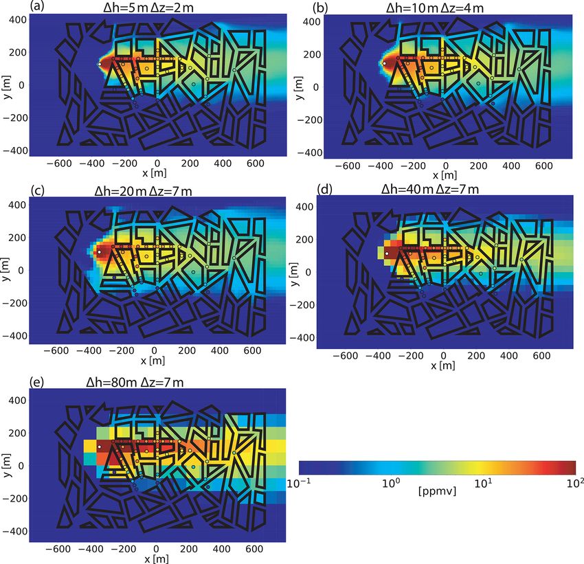
1470                                                                   M. Weger et al.: Urban dispersion model CAIRDIO

et al., 2013; Paas et al., 2016; Harrison, 2018). For an ac-      microscale approaches requires sufficiently fine grid spac-
curate simulation, it is thus not only key to explicitly repre-   ings. The landscape of microscale models is diverse (Fallah-
sent the urban canopy features but also to consider the pre-      Shorshani et al., 2017; Brown, 2014; Hanna et al., 2006)
vailing mesoscale meteorological conditions. Depending on         and it reflects the difficulty of finding a compromise be-
the level of physical detail, a trade-off in the use of high-     tween computational resources and accuracy. Computational
resolution numerical simulations is often their exclusive ap-     fluid dynamics (CFD) models can be seen as the microscale
plicability in a limited area, which can be very restrictive.     pedants to NWPs. Among them, LES approaches are the
Hence, an active topic of research is dedicated to improve        most accurate but expensive ones. LES models resolve the
the numerical efficiency of high-resolution modeling tools        turbulent spectra up to the filter cut-off size (often equivalent
and their incorporation into a larger modeling framework          to the grid size) and rely on simplistic subscale parameteri-
(Baik et al., 2009; Jensen et al., 2017; Kurppa et al., 2020).    zations only (e.g., Maronga et al., 2019). These two different
Commonly used multiscale approaches consist of nested do-         approaches (extensive parameterization vs. explicit represen-
mains and involve different types of models designed for          tation) are difficult to merge at the bridging scale range (few
a specific scale range. To address the global and regional        tens of meters to 1 km), for which reason Haupt et al. (2019)
scales, the use of chemistry transport models (CTMs) in           coined the keyword of “terra-incognita” to refer to the prob-
combination with numerical weather prediction (NWP) mod-          lem. An exemplary study, in which a LES model was applied
els is a well-established practice. Examples of those cou-        for horizontal resolutions up to above 100 m, is given by Ef-
pled model systems include the Integrated Forecasting Sys-        stathiou et al. (2016). However, their simulations did not in-
tem with chemistry (C-IFS; Flemming et al., 2015), the            clude an urban canopy, whose discretization would obviously
Weather Research and Forecasting model with chemistry             require a much finer grid. In fact, to fully resolve the energy-
(WRF-Chem; Grell et al., 2005), the Community Multi-              dominant eddies within street canyons, a spatial resolution
scale Air Quality model (CMAQ; Appel et al., 2017), the           of 15–20 grid points over a typical obstacle dimension size
ICOsahedral Nonhydrostatic model with Aerosols and Reac-          is needed (Xie and Castro, 2006). This translates in a grid
tive Trace gases (ICON-ART; Rieger et al., 2015), and the         spacing of about 1 m for typically sized buildings. The use
Consortium for Small-scale Modeling Multi-Scale Chem-             of such fine grids for entire city domains is still prohibitively
istry Aerosol Transport model (COSMO-MUSCAT; Wolke                expensive in LES modeling. For example, Wolf et al. (2020)
et al., 2004, 2012). In all of these models, subgrid-scale ef-    used a grid spacing of 10 m in their cutting-edge research
fects of temperature and moisture, as well as PBL dynam-          study to simulate air pollutant dispersion in Bergen, Norway,
ics, are parameterized. The influence of the urban canopy on      with the Parallelized Large-Eddy Simulation Model (PALM)
the PBL in NWP models can be considered through sophis-           model. While this spatial resolution, according to the argu-
ticated canopy parameterizations (Martilli et al., 2002; Schu-    ment above, does not ensure a LES model to be eddy resolv-
bert et al., 2012). The improvements of these so-called ur-       ing in every part of the domain, the preference of a physically
banized NWPs are substantially reflected in the modeled pol-      based model over the more widely used parameterized mod-
lutant concentrations (Kim et al., 2015; Wang et al., 2019).      els for this grid size (e.g., plume or street-canyon models)
Nevertheless, as the model domain does not allow for an ex-       can nevertheless be a legitimate choice. Resolved physics can
plicit representation of buildings, the pollutants emitted at     still be maintained outside the densely built urban canopy.
street level are diluted over the entire grid cell, which can     Within the canopy, the dispersion pattern on a larger scale
considerably deviate from real conditions, where a large part     is mostly shaped by the channeling and blocking effects of
of the physical volume may be impervious. As a result, pol-       buildings, which can be represented also with coarser grids.
lutant concentrations modeled using NWP-based approaches             In physical computing, it is well known that only a slight
are more representative of the urban background (Korhonen         increase in the grid spacing results in large computational
et al., 2019). Another practical limit to resolution and accu-    savings (e.g., models using explicit time integration ideally
racy of NWP models arises from the use of parameterizations       perform 16 times faster on the same domain using a grid
themselves. Using WRF, Haupt et al. (2019) observed that          with doubled grid spacings in all three dimensions). These
for horizontal grid spacings below the typical PBL height,        computational savings could in turn be spent in larger phys-
numerical results can become spurious. Based on their find-       ical domains for more comprehensive yet accurate urban-
ings, they recommend not to apply NWPs on the subkilome-          air-quality simulations. A key feature that sets the techni-
ter scale without careful replacement of the used parameteri-     cal limits to the spatial resolution in urban boundary-layer
zations. In PBL meteorology, the microscale seamlessly fol-       modeling is the discretization method used for obstacles.
lows the lower limit of the mesoscale (super-kilometer range)     A class of methods that allow for obstacle geometries not
(Stull, 1988; Rakai and Gergely, 2013). However, adopting         bound to the grid is the immersed boundary methods, sum-
the modeling perspective, there is a clear segregation of mi-     marized by Mittal and Iaccarino (2005). These are essen-
croscale and mesoscale. While the latter is constrained at the    tially Cartesian methods, but instead of relying on a com-
lower end of the resolution by the extensive use of parame-       monly used marker-and-cell method (grid cells are assigned
terizations, attempting to model PBL processes directly with      either to the building interiors or to the atmosphere), they

Geosci. Model Dev., 14, 1469–1492, 2021                                            https://doi.org/10.5194/gmd-14-1469-2021
M. Weger et al.: Urban dispersion model CAIRDIO                                                                             1471

represent rigid boundary conditions (e.g., Neumann bound-         benefits and limitations of the approach are summarized and
ary condition for pressure) on grid-cell faces not coinciding     concluded with an outlook for potential future applications.
with the obstacle boundary. Among these methods, the so-
called direct forcing uses the ghost-cell interpolation tech-
nique, where image points from adjacent interior ghost points     2     Model description
are mirrored across the rigid boundary and interpolated us-
                                                                  2.1    Basic equations
ing surrounding fluid nodes. While this method greatly en-
hances the flexibility in the choice of the grid size, it still   The physical domain consists of an interspersed, stationary
suffers from the empirical nature in the selection of the in-     solid phase representing the buildings and a mobile fluid
terpolation nodes and the interpolation method itself. On the     phase. The governing equations for the mobile phase are
other hand, an equivalent boundary forcing can be more rig-       deduced from a simplified two-phase model by neglecting
orously deduced from a two-phase flow model (Drew, 1983)          restoring forces. In a two-phase model, phase-fraction func-
by neglecting the restoring source terms. Treating one of the     tions α1 , α2 with 0 ≤ α1 ≤ 1 and α1 + α2 = 1 are used to for-
phases as an non-deformable solid, Kemm et al. (2020) de-         mulate the set of equations of both phases individually. The
rived a diffuse interface (DI) model for compressible flu-        equation of motion of an incompressible phase is adopted
ids. One of the main advantages of their approach is the          from Drew (1983) (Eqs. 41, 45 therein). By setting the inter-
algorithmic simplicity, as the boundary-forcing term is an-       facial force density and surface tension to zero, the simplified
alytically coupled to the DI, which is advected as a scalar.      momentum equation of the mobile phase (indicated with α1 )
In this work, we adopt the basic idea of DI and implement         is written as
diffuse obstacle boundaries (DOBs) in our new City-scale
AIR dispersion model with DIffuse Obstacles (CAIRDIO              ∂t (α1 ρu) = −∇ · (α1 ρu ⊗ u) − α1 ∇ (α1 p) + pI ∇α1
v1.0), which will be used as a computationally feasible yet           + ∇ · (α1 T) + α1 ρb.                                    (1)
accurate downscaling tool for mesoscale air pollution fields
over urban areas. DOBs allow buildings to be represented              Here, the 3-D velocity vector is denoted by u, and ρ is
as diffuse features, and thus the flexibility in the choice of    the density of air and pI the interface pressure, which reflects
grid resolution can be greatly increased. A DOB is a sim-         Newton’s third law of motion near a fixed wall. As in Kemm
plified form of DI resulting from the static boundaries as-       et al. (2020), pI is assumed to be in equilibrium with the sur-
sociated with buildings. A DOB is incorporated in the dis-        rounding fluid pressure p. The stress tensor T contains the
crete differential operators by considering the conservation      contributions from subscale and surface fluxes in LES aver-
laws in a finite volume framework. The equations are then         aging. In this model, the implicit approach is used for spatial
solved with standard methods on a Cartesian grid. To inter-       filtering (Schumann, 1975). Viscous stresses are neglected
pret our DOB approach from a physical point of view, it can       due to the high Reynolds numbers typically encountered in
be argued that the grid cells are interspersed with a porous      atmospheric flows. The sum of external body forces b con-
and semi-permeable medium. Their detailed structure is only       tains the gravitational force and inertial forces resulting in
of concern insofar as it determines the mass and momentum         a rotating frame of reference. The interface in our case is
budged at the grid level through two different types of in-       static, as buildings do not respond to the flow. This makes it
terface fields. To the authors’ knowledge, this approach has      possible to multiply the equation of motion with α1−1 ρ −1 to
not been used for air-quality modeling so far, but very in-       obtain the tendency equation in single-flow denotation. The
terestingly the concept of permeability finds application in      reference density ρref is kept constant in time for an incom-
geological science (Haga, 2011). In contrast to geometry-         pressible fluid. The full set of model equations reads
aligned discretizations, which preserve a high degree of ac-
curacy near obstacle walls but require high resolutions, this                                     1 −1
                                                                  ∂t u = −α1−1 ∇ (α1 u ⊗ u) −        α α1 ∇p − α1−1 ∇
approach is more suited for the integral aspect of building                                      ρref 1
shapes and configurations at marginal resolutions. However,                                   2v − 2v
by increasing the grid resolution, the approach seamlessly            · (α1 T) − f × u + g              ,                      (2)
                                                                                                2v
transitions to a traditional obstacle-resolving Cartesian ap-
proach, as the interface eventually becomes sharply defined       α1−1 ∇ · (α1 u) = 0,                                         (3)
and imposes Neumann boundary conditions on the pressure.          ∂t 2 = −α1−1 ∇ · (α1 u2) + α1−1 ∇ · (α1 kh ∇2) + α1−1 S2 ,   (4)
   The paper is organized as follows: Sect. 2 provides a de-
                                                                  ∂t Qv = −α1−1 ∇ · (α1 uQv ) + α1−1 ∇ · (α1 kh ∇Qv )
tailed description of the model CAIRDIO, including the spa-
tial discretization method. Section 3 contains numerical tests       + α1−1 SQv ,                                              (5)
to demonstrate the diffuse obstacle discretization, the dy-       2v = 2 (1 + 0.61Qv ) .                                       (6)
namic core, and the parallel scaling capabilities. In Sect. 4,
we present a model-evaluation study by simulating a realis-         In the momentum equation (Eq. 2), the body-force term is
tic wind-tunnel dispersion experiment. Finally, in Sect. 5, the   replaced by the Coriolis term, with the Coriolis parameter f

https://doi.org/10.5194/gmd-14-1469-2021                                             Geosci. Model Dev., 14, 1469–1492, 2021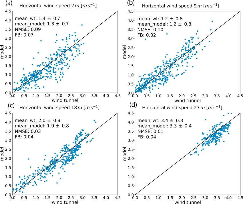
1472                                                                        M. Weger et al.: Urban dispersion model CAIRDIO

for a mean geographic latitude, and the buoyancy term using        pressure equation:
the Boussinesq approximation. g is the gravity-acceleration
vector in the local frame of reference and 2v the virtual po-      4 =4̃ − ∂x (∂x h∂z ) − ∂y ∂y h∂z − ∂z (∂x h∂x )            (12)
tential temperature defined by Eq. (6). The overbar denotes
                                                                                           h         i    h        i
                                                                      − ∂z ∂y h∂y + ∂z (∂x h)2 ∂z + ∂z (∂y h)2 ∂z .

the horizontal mean state. Equation (3) is the continuity equa-
tion derived in an analogous way to the momentum equation
                                                                      As u, v, and w are maintained as the prognostic model
from the original formulation in Drew (1983). The transport
                                                                   variables and g is invariant under the given coordinate trans-
equation for scalars, like the potential temperature 2 and
                                                                   formation, no metric terms arise in the buoyancy term. How-
specific humidity Qv , contains source terms from parameter-
                                                                   ever, the horizontal averaging of 2v is carried out on z isosur-
ized surfaces fluxes. These have to be multiplied with α1−1 .
                                                                   faces. Therefore, 2v is remapped to an auxiliary vertical grid
The scalar field kh is the eddy-diffusion coefficient for heat.
                                                                   and the calculated tendency is remapped back to the compu-
Note that the combinations α1−1 ∇ · α1 and α1−1 α1 ∇ can be
                                                                   tational grid.
identified as particular versions of the divergence and gradi-
ent operator, which incorporate diffuse boundaries. Using a        2.3      Diffuse obstacle boundaries
staggered grid, the stencil of α1 (face centered) differs from
α1−1 (volume centered), so that the terms do not cancel each       The spatial discretization uses a finite volume method, which
other out.                                                         allows a consistent treatment of the diffuse obstacle bound-
                                                                   aries. To consider the conservation of a scalar q within two
2.2    Computational grid                                          partitioned phases, the Gauss theorem is formulated for a sin-
                                                                   gle grid-cell volume 1V and its total surface area ∂1V :
The computation uses a structured Arakawa-C grid, with             Z
the velocity components being defined at the cell faces and
                                                                      ∂t qm χm + qs (1 − χm ) dV 0 =

scalar fields at the cell centers. Vertical coordinate transfor-
mation allows for a curvilinear grid in the physical space to      1V
                                                                             Z
be adapted to a smoothly varying terrain function:
                                                                                      ηm · um qm + (1 − ηm ) · us qs dA0 .

                                                                        −                                                     (13)
x̃ = x,   ỹ = y,   z̃ = z − h(x, y).                       (7)             ∂(1V )

  Here, z is the mean sea level height and h(x, y) the terrain-        Here, subscript m refers to the mobile phase and subscript
height function. Elevated levels are simply given by adding a      s to the solid phase for the building interior. A0 and V 0 are
horizontally constant vertical increment to the first level.       formal integration variables. χm is the volume-fraction func-
  The pressure gradient in terrain-following coordinates is        tion of the mobile phase and ηm the area-fraction function,
modified to                                                        over which the flux of the mobile phase is integrated. As al-
                                                                   ready mentioned, the stationary solid phase is dropped, as
     ˜ − ∂x h(x, y) + ∂y h(x, y) ∂z p.
∇p = ∇p

                                                            (8)    it is ∂t χm = 0, ∂t qs = 0 and us = 0. This simplifies the con-
                                                                   servation form and finally leads to the particular differential
   The divergence operator is applied on the contravariant         form of the transport equation for the mobile phase:
velocity components, which are parallel to the cell-face nor-                    1
                                                                                         Z
mal. In our simple case, only the vertical contravariant veloc-    ∂t q m = −                ηm · um qm dA =
                                                                               χm 1V
ity component ω differs from the covariant non-transformed                                 ∂(1V )
component. It is given by
                                                                           1
                                                                        −    ∇ · ηm (um qm ) =: −∇m · (um qm ).               (14)
ω = w − ∂x hu − ∂y hv.                                      (9)           χm
                                                                     The subscript m was only briefly introduced here and will
   Using Eq. (9), the advective tendency of a scalar q is writ-    be dropped again, as only the mobile phase is of interest.
ten as                                                               Using the Cartesian grid structure, the discrete flux diver-
                                                                 gence results from
∂t q = −u∂x q − v∂y q − w − u∂x h − v∂y h ∂z q.            (10)
                                                                                   1
  Similarly, the continuity equation in terrain-following co-      ∇ ·F =             [(ηx 1Ax Fx )L − (ηx 1Ax Fx )R          (15)
                                                                                 χ 1V
ordinates follows from
                                                                                         + (ηy 1Ay Fy )L − (ηy 1Ay Fy )R
∂x u + ∂y v + ∂z (w − ∂x hu − ∂y hv) = 0.                  (11)                          + (ηz 1Az Fz )L − (ηz 1Az Fz )R ],

  Combining Eqs. (11) and (8), the metric terms in the             where 1V and 1Ax,y,z are the cuboid volumes and face ar-
Laplace operator are obtained, which is later needed for the       eas, respectively. The superscripts R and L refer to the left

Geosci. Model Dev., 14, 1469–1492, 2021                                                   https://doi.org/10.5194/gmd-14-1469-2021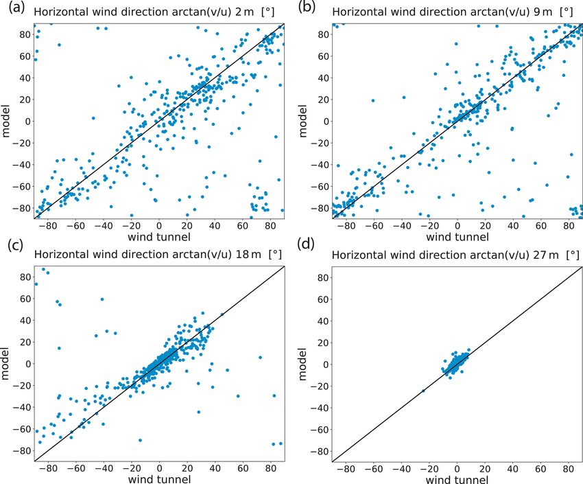
M. Weger et al.: Urban dispersion model CAIRDIO                                                                                     1473

and right cell faces for each dimension, respectively. Fx , Fy ,
and Fz are fluxes whose concrete form is determined by the
partial differential equation. Note that the contravariant flux
has to be used for Fz .
   The pressure-gradient components on the cell faces are
discretized with second-order accuracy. The gradient com-
ponents centered on the x- and z-oriented cell faces, respec-
tively, are

             2ηx 1Ax
                            pR − pL

∂x p =         L          R
        (χ 1V ) + (χ 1V )
       1
           hR − hL Lz→x ∂z p,

    −                                                       (16)
      1x
             2ηz 1Az
                            pR − pL ,

∂z p =         L         R
                                                            (17)
       (χ 1V ) + (χ 1V )                                            Figure 1. (a) Depiction of two different building sections (gray-
                                                                    filled areas) inside a grid cell. The black lines mark the effectively
where    Lz→x is the linear interpolation operator from a z face
                                                                    blocked area of the respective side. The line pattern symbolizes the
to an x face, and 1x is the cuboid size used for differencing       slicing of the grid-cell volume, which is shown here only for the
the terrain function.                                               x dimension. (b) Scaling factors for a complete building, now de-
   For a grid-conform surface, the area fractions ηx,y,z =          picted as fields calculated for three different grid resolutions. χ is
0, from which the required homogeneous zero Neumann                 the volume-scaling field, and ηx , ηy are the horizontal components
boundary condition follows. In this case, a grid cell is com-       of the area-scaling field.
pletely surrounded by grid-conform surfaces and the pres-
sure value inside is decoupled from any neighboring values,
reflecting its physical meaninglessness. For partially open         occasionally, a cell face is assigned to both values from the
semi-permeable cell faces, the boundary condition is im-            adjacent left and right grid cells, respectively, the minimum
posed on a fraction of the cell face area only.                     of both values is taken. For the resulting cell face left with-
   The scaling fields ηx,y,z and χ are derived from geomet-         out assignment, the geometric intersection with buildings is
ric building data. As an alternative to using terrain-following     calculated as in the resolved case. Figure 1b demonstrates
coordinates, it is possible to use diffuse boundaries for the       that this method preserves the blocking effect of a triangular-
terrain, in which case, the subsurface is also represented by       shaped building for spatial resolutions, which are too coarse
a geometric shape. Per definition, the volume-fraction field        to resolve individual building walls.
χ is expressed as the fraction of the obstacle-free volume in
each grid cell. For numerical reasons, however, χ is limited        2.4     Numerics
to a small non-zero value. For well-resolved buildings, the
area-scaling fields ηx,y,z are derived by calculating the inter-    2.4.1    Advection scheme
sections of the buildings with the grid-cell faces. For under-
                                                                    The advective tendency for a scalar q is obtained by adding
resolved buildings, however, this method fails to take the grid
                                                                    the remnant velocity-divergence term from the approximate
alignment into account. A resulting effect may be the entire
                                                                    pressure solution to the flux-divergence term of the conser-
missing of buildings if they do not intersect with a particular
                                                                    vation law (Eq. 15):
cell face but nevertheless block the flow within a grid cell.
Figure 1a shows two possible scenarios, where grid cells are        (∂t q)adv = −∇ · (uq) + q∇ · u.                                  (18)
intersected by a building, which obviously blocks the flow
in one dimension completely but does not intersect with the            The flux components are linear and given by the product of
cell faces oriented in the direction of the blocking. In order to   the reconstructed values q̃ at cell faces and the exactly given
capture such occurrences more reliably, a modified method to        momentum components. We use an upwind-biased stencil of
calculate the area fractions is used. In this method, the grid-     fifth order, which results in two reconstructions (q̃ + and q̃ − )
cell volume is partitioned in slices, with the slicing planes       on each cell face. For an x-oriented face, the reconstructions
being displaced along the dimension considered (e.g., the x         are merged to the numerical flux by considering the wind
dimension for yz faces). The minimum value over the free-           direction:
volume fractions of all slices is computed to define a cell-
                                                                    (uq)x = 0.5 ux (q̃ + + q̃ − ) − ||ux ||(q̃ + − q̃ − ) .

area-scaling factor, which is then assigned to the cell face in                                                                 (19)
closer proximity to the obstacle. For a more robust capture
of non-parallel building walls, the slicing can be repeated           For non-uniform grid spacings, the coefficients of the re-
several times with a slight rotation of the plane normal. If,       construction polynomials are precomputed from the spatial

https://doi.org/10.5194/gmd-14-1469-2021                                                Geosci. Model Dev., 14, 1469–1492, 2021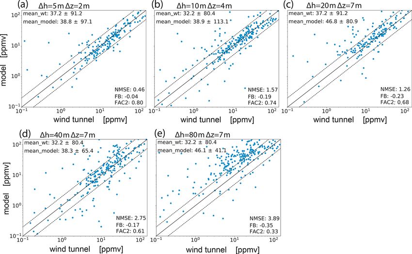
1474                                                                             M. Weger et al.: Urban dispersion model CAIRDIO

                                                                         2.4.2    Model integration

                                                                         In the incompressible-flow equations, the pressure-gradient
                                                                         term is not directly coupled to a prognostic pressure equa-
                                                                         tion. The projection method of Chorin (1968) is used to split
                                                                         the solution procedure in two steps. The first step integrates
                                                                         all the momentum tendencies, except the stated pressure-
                                                                         gradient term, explicitly in time to obtain a predicted velocity
                                                                         ũ:
Figure 2. (a) Plot of the pseudo-grid spacing 1eff  x computed for
a solid cylinder with diameter of 10 m using a uniformly constant        ũ = ut0 + (∂t u)ex |t0 1t.                                 (21)
grid spacing of 1 m. Decoupled cells inside the cylinder are charac-
                                                                           The final velocity estimate after one integration step ut1
terized by 1eff                                         eff
             x > 2 m in this plot. (b) Using same 1x of (a), the
reconstruction coefficients are computed for a five-point upwind-
                                                                         has to fulfill the continuity equation:
biased stencil. The absolute values of the reconstruction coefficients
                                                                         ∇ · ut1 = 0.                                                (22)
are re-normed to 1 and depicted in shades of gray at individual re-
construction sites, which are marked by a vertical red bar. Stencil         The required corrective tendency has to be associated with
points are rendered invisible for values below 10−4 and as such
                                                                         the neglected pressure gradient, which is formally integrated
have a negligible influence on the reconstructed value.
                                                                         with an Euler-backward step to obtain the final velocity at
                                                                         t1 = t0 + 1t :
derivative of the Lagrange polynomial which interpolates the                          1t
primitive function at cell faces (see, e.g., Shu, 1998). We use          ut1 = ũ −        ∇|pt1 .                                   (23)
                                                                                      ρref
the pseudo-grid spacing calculated by 1eff                   L
                                              x = 21x χ /(ηx +
  R
ηx ) instead of the computational grid spacing in order to au-             By applying the divergence operator on both sides and re-
tomatically adjust the effective stencil width near obstacle             quiring that ∇ · ut1 = 0, the well-known Poisson equation for
boundaries. The behavior of the pseudo-grid-based recon-                 pressure is obtained:
struction of maximum fifth order is demonstrated in Fig. 2 for           ρref
a positive flow direction (left to right). Within the shown cir-              ∇ · ũ = 4p|t1 .                                       (24)
                                                                         1t
cular obstacle, the pseudo-grid spacing tends toward infinity,
which effectively excludes such decoupled cells from inter-                 After algebraic solution of this equation, the final state can
polation. The resulting smaller stencils can be downwind bi-             now be composed of the fractional tendencies:
ased. An effective measure to prevent numerical instabilities
                                                                                                         1

is the application of a flux limiter (e.g., from Sweby, 1984)            ut1 = ut0 + 1t (∂t u)ex |t0 −      ∇p|t1 .                   (25)
                                                                                                       ρref
near obstacle boundaries. To avoid non-physical results of
positive scalars, a limiter has to be applied anyway. In the                Equation (25) is only first-order accurate in time. For
case of momentum advection, we use the absolute difference               higher accuracy, it is instead used a third-order strong-
|ηx (j − 1) − ηx (j )| as a weighting function to merge the lim-         stability-preserving Runge–Kutta scheme (SSP-RK3) for the
ited and unlimited reconstructions for obstacle-specific lim-            advective and pressure-gradient tendencies, which also al-
iting. Note that this expression is upwind-biased (assuming a            lows us to use larger time steps. The pressure to correct the
positive wind direction). In the free boundary layer, the dif-           first two intermediate states is extrapolated from values given
ference is zero and no limiting is applied. The routine for              at previous time steps, and only for the final stage, the pres-
scalar cell-centered advection is repeatedly used to advect              sure solver is applied (Karam et al., 2019). We found that
a left-faced ul and right-faced value ur for each momentum               this combination supports stable integration up to a Courant
component (Hicken et al., 2005; Jähn et al., 2015), resulting            number of C = 0.7.
in a total of six advection steps. The final momentum tenden-
cies are obtained by interpolation of two centered tendencies            2.4.3    Pressure solution
on the face:
                         R                 L                           The discretization of the Laplace operator P in the Poisson
  adv       χ 1V ∂tadv ul + χ 1V ∂tadv ur                                equation (Eq. 24) is obtained by the product of the discrete
∂t u =                                         .            (20)         divergence D and gradient in sparse matrix form. D is defined
                  (χ 1V )R + (χ 1V )L
                                                                         by the flux balance in Eq. (15). Combining the operators to
  Spatial accuracy of momentum advection is limited to the               the pressure equation, the following sparse linear system is
order of this interpolation procedure, which is of second or-            obtained:
der here.
                                                                                  1
                                                                         Pp =        Dũ =: b,                                       (26)
                                                                                  1t

Geosci. Model Dev., 14, 1469–1492, 2021                                                     https://doi.org/10.5194/gmd-14-1469-2021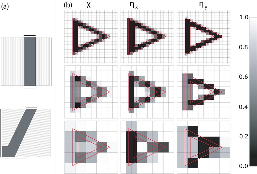
M. Weger et al.: Urban dispersion model CAIRDIO                                                                             1475

where ũ, p, and b are the one-dimensional expanded ar-           the already updated boundary values should not be changed
rays of the corresponding structured fields. Equation (26) is     by the projection:
solved with a geometric multigrid method in parallel using
domain decomposition in two dimensions. The multigrid al-                    ∂ ũ
                                                                  0 = ρref        · n = ∇p · n.                              (28)
gorithm consists of applying a smoothing method of choice                    ∂t
which is accelerated by coarse-grid corrections. Therefore,
                                                                     Here, n is the unit normal vector on the boundary surface.
a hierarchy of coarse grids is employed (Brandt and Livne,
                                                                  A more general case arises with the use of terrain-following
2011). A 3-D coarsening of the grid is carried out by ag-
                                                                  coordinates. By requiring not only ∂t ω = 0 but additionally
glomeration of eight grid cells to form a coarse-grid cell of
                                                                  ∂t w = 0 at the bottom and top of the computation domain,
the next-level grid. For uneven grid sizes, a plane of grid
                                                                  the following boundary condition follows at these bound-
cells with respective orientation is left uncoarsened. This
                                                                  aries:
particular multigrid used in combination with finite volume
discretizations is often referred to as a cell-centered multi-    ∂z p = 0                                                   (29)
grid in literature (Mohr and Wienands, 2004). Particular                 (
challenges to the multigrid algorithm include grid stretch-                0             ∂x h 6 = 0
                                                                  ∂x p =
ing and, in our case, non-smoothly varying coefficients as-                not specified else
sociated with the diffuse boundaries, both resulting in co-              (
efficient anisotropy. An odd grid size results in coefficient              0             ∂y h 6 = 0
                                                                  ∂y p =                                                     (30)
anisotropy of the coarse-grid operators. In such cases, plane              not specified else.
smoothers are often much more robust than their point-wise
pendants (Llorente and Melson, 2000). Nevertheless, most of          In the discrete gradient operator, homogeneous Neumann
the difficulties could be overcome by applying less elaborate     boundary conditions are implemented by setting all coeffi-
methods in the current model. Based on smoothing analysis,        cients associated with the node to zero where the condition
Larsson et al. (2005) give a condition for the optimal loca-      applies.
tion of an uncoarsened plane in the case of an odd grid size.        The boundary condition for the velocity field has to be
Galerkin coarse-grid approximation can result in a better ap-     compatible with a dynamic mesoscale forcing and also sat-
proximation of the coarse-grid operator in this case, while       isfy Eq. (27). Firstly, inflow and outflow regions are dynam-
discretization coarse-grid approximation can be more effi-        ically determined in order to impose separate appropriate
cient for even-sized grid dimensions. Our algorithm employs       boundary conditions. Outflow regions are characterized by
a combination of both methods on different grid levels.           convective transport out of the domain. Therefore, a sim-
                                                                                                                      1t
   Yavneh (1996) found that for smoothing, successive over-       ple normalized convective transport speed (C⊥ = 1x     u · n) is
relaxation (SOR) is generally superior to Gauss–Seidel            computed. Note that more elaborate formulations for C⊥ ex-
smoothing (even for isotropic coefficients), and he also de-      ist. C⊥ is further bounded to [0, 1] for numerical reasons. It
rived approximately optimal over-relaxation factors for SOR       is then C⊥ > 0 for outflow regions. For such regions, the ra-
with red–black ordering applied in multigrid for the solution     diation boundary condition by Miller and Thorpe (1981) is
of anisotropic elliptic equations. In our implementation, also    imposed:
sparse-approximate inverse (SPAI) matrices (Tang and Wan,           t+1
                                                                        = utl+1 − C⊥ utl+1 − utl .

2000; Bröker and Grote, 2001; Sedlacek, 2012) are available       ul+1                                                       (31)
as suitable alternatives to SOR. These smoothers can inher-
ently consider coefficient anisotropy through the algebraic          The order of the spatial indexing l is in normal direction
method by which they are derived. Moreover, a variable num-       to the boundary and not to be mixed up with the standard in-
ber of non-zeros in the matrix allows a flexible control of the   terior indexing. The index l + 1 corresponds to the first ghost
approximation quality and smoothing efficacy.                     cell. At the remaining inflow boundaries, Dirichlet condi-
                                                                  tions are specified.
2.4.4   Lateral boundary conditions                                  Instead of this flexible inflow–outflow boundary condition,
                                                                  a Rayleigh damping layer can be used as another prognostic
Before each pressure correction step, lateral boundary con-       tendency near the domain top:
ditions of the intermediate velocity field ũ are updated. The
                                                                   dmp          R(z)
update has to ensure global mass conservation:                    ∂t     q =−        (q − q0 ).                              (32)
                                                                                 τ
I
   ρref
        ũ · n dA0 = 0.                                    (27)      Equation (32) can be applied to gradually relax any prog-
    1t                                                            nostic variable toward a prescribed horizontal mean state at
∂V
                                                                  the top boundary. R is a ramp function with values between
  This expression implies a homogeneous-zero Neumann              [0, 1], τ the damping timescale, and q0 the prescribed bound-
boundary condition for pressure at all lateral boundaries, as     ary value.

https://doi.org/10.5194/gmd-14-1469-2021                                               Geosci. Model Dev., 14, 1469–1492, 2021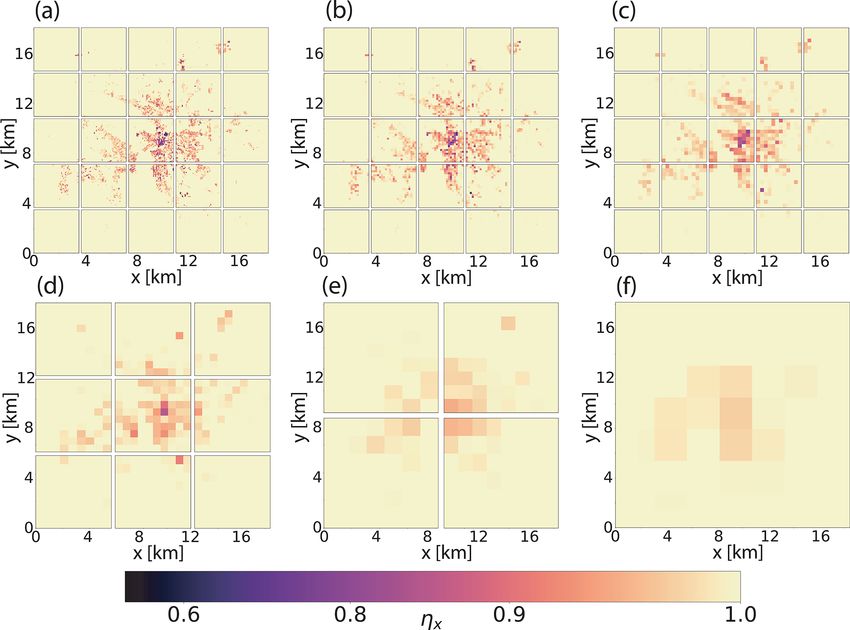
1476 M. Weger et al.: Urban dispersion model CAIRDIO
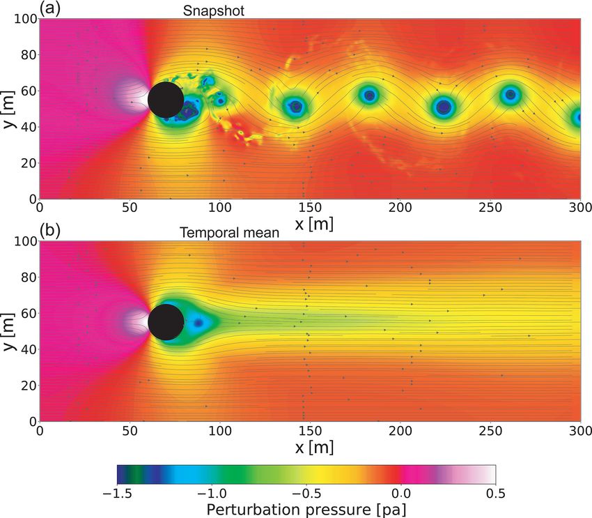
Figure 3. Example of a horizontal multigrid domain decomposition involving six grid levels. Depicted are the area-scaling factors of yz
faces for the city of Leipzig at resolutions of (a) 80, (b) 160, (c) 320, (d) 640, (e) 1280, and (f) 2560 m. The scaling factors are needed in the
discretization of the Poisson equation. On the coarsest grid, a single processor is left for the computation.
Final mass conservation is enforced by making sure that numbers, the principal purpose of the subgrid model is to
the total inflow–mass flow is exactly balanced by the total dissipate enough energy at the shortest wavelengths to ob-
outflow–mass flow. This is accomplished by computing an tain a physically realistic energy cascade. In our case, the
averaged correction velocity from the mass-flow difference. subgrid model also has to compensate for the under-resolved
In the case, each spatial dimension is considered indepen- vertical mixing of tracers within the urban boundary layer.
dently from each other, this results in three different correc- In the Smagorinsky model, the rates of strain sx,y are approx-
tion velocities. The correction velocities are finally added to imated by the velocity gradients:
the boundary-perpendicular velocity component at the out-
flow regions. 1
sx,y = ∂y u + ∂x v . (33)
Figure 4 shows that the outflow boundary condition with 2
the proposed convective transport speed is well suited to our The subscripts x, y refer to the spatial components. The tur-
incompressible model even for highly unsteady flows, like bulent fluxes are derived in analogy to the viscous fluxes by
the depicted vortex street in the wake of a cylinder. Individ- assuming an eddy viscosity k :
ual vortices are not visibly reflected at the boundary, and also
in the temporal mean, based on Fig. 4b), the influence of the u0x u0y = 2x,y sx,y . (34)
boundary is not noticeable. The flexible boundary condition
can principally be applied to any other scalar quantity, al- The often additionally mentioned anisotropic residual-
though, specifying Dirichlet conditions for advected scalars stress tensor is ignored in the given incompressible case. In
was found to be well suited. the most simple case, x,y is also diagnosed from the rates
of strain. x,y is denoted in tensor form, as an anisotropic
mixing length lx,y is used to reflect grid anisotropy:
2.5 Physical processes
2
2
x,y = lx,y |S|f = cs 1x,y |S|fs . (35)
2.5.1 Subgrid model
|S| is the Frobenius norm of the strain-rate tensor. cs is the
For numerical simplicity and efficiency, a static Smagorin- Smagorinsky constant, which is fixed in a static model. Tests
sky subgrid model is used (Deardorff, 1970). Since the at- with a boundary-layer simulation revealed that the range
mospheric model is operated in the limit of infinite Reynolds 0.1 < cs < 0.15 gives good results in combination with the
Geosci. Model Dev., 14, 1469–1492, 2021 https://doi.org/10.5194/gmd-14-1469-2021
M. Weger et al.: Urban dispersion model CAIRDIO 1477
the divergence of the diffusive fluxes. Shifted grids are in-
troduced to account for the definition of the velocity com-
ponents on the cell faces. For example, diffusion of the
u component requires a grid shifted by 1x /2, for which
the scaling fields are also obtained by linear interpolation.
The diffusive fluxes are given by
Fx,y = 2x,y sx,y . (39)
For diffusion of the u component, the fluxes in the three
spatial directions are Fx,x , Fx,y , and Fx,z . Those of the other
components are obtained by permuting the subscripts. For
a scalar quantity q, the required fluxes are Fx,x , Fy,y , and
Fz,z , with the rates of strain being replaced by the gradient
components.
2.5.2 Surface fluxes
Surface fluxes for momentum, heat and moisture are pa-
Figure 4. LES of 3-D flow past a cylinder. The horizontal grid spac- rameterized using Monin–Obukhov similarity theory (Louis,
ing is uniformly 0.5 m. The cylinder has a diameter of 40 m. The 1979). An expression for the vertical transfer coefficient Cz
approaching flow is laminar with u = 1 m s−1 . Flexible Dirichlet- can be obtained by transforming the logarithmic wind law:
radiation conditions are imposed on all horizontal domain bound-
aries, while periodic boundary conditions are used in the z direc- k2
Cz = . (40)
tion. The contour plot depicts the pressure and the streamlines the log2 (z/z0 )
horizontal velocity field. Panel (a) shows a frame at the instance
during a sharply defined vortex is about to cross the right boundary; k = 0.4 is the Von Kármán constant, z0 the surface roughness
panel (b) shows the temporal mean over a representative simulation length, and z the height difference from the modeled surface
period. to the grid level where the parameterization is evaluated.
The momentum sinks from horizontal surfaces are
fifth-order upwind scheme. Grid anisotropy enters via 1x,y , ∂u0 w0 Az p
=− fm Cz u u2 + v 2 (41)
which is further modified by half the mean distances to walls ∂z 1V
hx and hy , respectively:
and
p
1x,y = min 1x 1y , 1.8hx , 1.8hy . (36) ∂v 0 w0 Az p
=− fm Cz v u2 + v 2 . (42)
∂z 1V
Function fs introduces the influence of the stratification on
the eddy viscosity. It is assumed that Analogously, the source terms for heat and moisture from
horizontal surfaces are
0
Ri ≥ 0.25
√ ∂20 w 0 Az p
fs = 1 − 16Ri Ri < 0 (37) =− fh Cz 2 − 2s u2 + v 2 (43)
4 ∂z 1V
(1 − 4Ri) else,
and
with the Richardson number Ri:
∂Q0v w 0 Az p
g∂z 2v =− fh Cz Qv − Qsv u2 + v 2 . (44)
Ri = . (38) ∂z 1V
2v |S|2
2s is the surface potential temperature, and Qsv the surface
For scalar diffusion, the eddy viscosity is divided by the specific humidity. Az is the total exposed horizontal surface
turbulent Prandtl number, which is assumed to be P r = 2/3 within the grid cell, and 1V the effective cell volume. fm
here. and fh are stability functions, and z0 is the surface roughness
If not mentioned otherwise, the appearing spatial deriva- length. We adopt the expressions given in Doms et al. (2013)
tives are discretized with second-order differences. To obtain to calculate fm and fh for land surfaces. Sources and sinks
the strain-rate components and the eddy viscosity on dif- from vertical building walls are treated similarly, but the sta-
ferent stencil points (cell faces areas and cell centers), lin- bility function is set to unity in this case. For x-oriented sur-
ear interpolation is used. The subgrid tendency is formed by faces, z is replaced by half of the average distance between
https://doi.org/10.5194/gmd-14-1469-2021 Geosci. Model Dev., 14, 1469–1492, 2021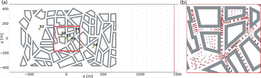
1478                                                                         M. Weger et al.: Urban dispersion model CAIRDIO

surfaces in the equation for the transfer coefficient. Analo-         2.6    Programming language
gously, Az is replaced by Ax for the total projected surface
area with x orientation. The surface fields 2s and Qsv are            The presented model (CAIRDIO v1.0) is written in Python,
part of the external forcing and have to be provided either by        a programming language which facilitates a straightforward
the hosting mesoscale model or field-interpolated measure-            implementation of numerical methods, code compactness,
ments.                                                                and code readability. Python packages like NumPy, SciPy,
                                                                      and mpi4py make the programming language also suitable
2.5.3   Turbulence recycling scheme                                   for high-performance computing. Our model implementation
                                                                      can particularly benefit from NumPy, as all time-critical nu-
Wu (2017) gives an overview of various turbulence genera-             merical routines (e.g., all the routines for the computation of
tion methods to provide turbulent inflow conditions. Among            explicit tendencies) support vectorized computations. This is
the different methods, a turbulence recycling scheme is used          an inherent property of the diffuse interface approach, as all
in our model, as it is computationally efficient and can be           grid cells, except for the ghost cells at subdomain bound-
applied to a wide range of different domains and flow types.          aries, are computation cells and treated in the same manner.
In our implementation, turbulence can be extracted within             All tendencies are formulated in flux-divergence form, and as
a maximum of four vertical planes, each one properly dis-             a result, obstacle boundaries do not have to be specified par-
placed parallel to a particular inflow boundary. The resulting        ticularly. For the multigrid pressure solver, SciPy provides
domain fetch for turbulence recycling has to extend several           efficient data structures, methods, and functions for sparse-
integral length scales in order to prevent a spurious periodic        matrix algebra. Parallel computation is realized through a 2-
pattern of the recycled turbulent features.                           D domain decomposition, with each processing node running
   At each model time step, a horizontal filter is applied on         its own full-fledged simulation. Message Passing Interface
the velocity components within the recycling plane. In the            (MPI) is used to successively exchange data between subdo-
case of coupling with a mesoscale model, the filter width wr          mains.
is set to just below the spatial resolution of the host model
in order to spare mesoscale variations. Vertical filtering is
not feasible due to the strong vertical wind shear within the         3     Numerical tests
boundary layer. The filtered velocity component is subtracted
from the original one to obtain the small-scale fluctuation           Some numerical tests are conducted in order to examine grid
component:                                                            sensitivity of the diffuse obstacle interface, the dynamic core,
                                                                      and parallel efficiency of the model. To test the diffuse ob-
u(z, y)0 = u(z, y)− < u(z, y)>wr .                            (45)    stacle interface, a similar advection test as reported in Cal-
                                                                      houn and LeVeque (2000) is performed. In order to show that
   Equation (45) assumes a boundary perpendicular to the              the dynamic core can reproduce the expected evolution of an
flow in the x direction. The turbulent intensity is rescaled          idealized setup, the rising-bubble experiment of Wicker and
to the target value, after which the fluctuation field can be         Skamarock (1998) is conducted once again. It also provides
added to the inflow boundary field uin of the large-scale flow        a benchmark to compare the anelastic approximation with a
uls .                                                                 fully compressible model used in the original study. Finally,
                                                                      a third test is conducted to demonstrate the strong scalability
                                     ||u0tar ||2 (z) 0                on a high-performance computing platform.

uin (z, y) = uls (z, y) + min amax ,                  u (z, y) (46)
                                      ||u0 ||2 (z)
                                                                      3.1    Advection through an obstacle field
amax is used to limit the artificial amplification of turbulence
shortly after model initialization.                                   In this 2-D test, the computation domain contains randomly
   The filtering operation as well as the calculation of the          positioned circular obstacles of varying size. In a first step, an
turbulent intensities require communications in the parallel          approximate potential flow solution is computed. Therefore,
implementation. For optimal parallel scaling, filtering is per-       one step of the pressure projection method is applied on the
formed on each subdomain containing a part of the recycling           initial wind field defined by u = 1 and v = 0. The resulting
plane instead of the much simpler method of filtering all the         potential flow field is used to advect a test-tracer front, which
data with a single processor. A box-shaped filter is used to          is solely characterized by the left inflow boundary condition:
minimize the amount of communication in the parallel fil-                   (
tering. A final communication may be necessary to transfer                   1   t ≤ 40 s
                                                                      c=                                                           (47)
the recycled turbulence to the inflow boundary. Despite the                  0   t > 40 s.
communication-intense filtering, the computational costs of
the recycling scheme were found to be 1 % to 2 % of total                For the transversal-flow direction, periodic boundary con-
costs on average.                                                     ditions are used.

Geosci. Model Dev., 14, 1469–1492, 2021                                                https://doi.org/10.5194/gmd-14-1469-2021
M. Weger et al.: Urban dispersion model CAIRDIO 1479
Figure 5. Results of the advection test with obstacles. Map plots of the concentration field of a test tracer after a simulation time of 150 s.
The obstacles are drawn by contours of the volume-scaling field χ. Shown are the results of the flow simulations for the grids (a) 200 × 100
cells, (b) 100 × 50 cells, (c) 50 × 25 cells, and 25 × 13 cells, respectively.
spatially averaged concentrations at the outflow boundary vs.
time. For the case with the finest grid, the concentrations at
the outflow boundary start to rise after t = 145 s and peak at
about t = 185 s. At t = 250 s, most of the wave is advected
out of the domain. Remarkably, as already found by Calhoun
and LeVeque (2000), the washout curve is not sensitive to the
grid resolution up to 4 m, which is at the transition when ob-
stacles start to become diffuse. For the case with the coarsest
resolution of 8 m, the peak is slightly broader, peak concen-
trations are lower, and the peak occurs earlier by about 5 s.
At this grid resolution, the numerical diffusion of the advec-
tion scheme becomes important, as the resolution capability
is around six grid points, which is barely enough to resolve
the wave.
Figure 6. Washout curves of the test tracer for the different grid
resolutions in Fig. 5. The values are computed by integrating over 3.2 Rising thermal
the modeled outflow at the downwind (right) domain border.
In the rising thermal simulation described in Wicker and
Skamarock (1998), the Euler equations without diffusion are
solved on a 2-D domain with a height of 10 km and a width
The reference simulation is carried out on a domain with
of 20 km. The grid spacing is uniformly 125 m. The initially
200 × 100 grid cells and a uniform grid spacing of 1 m. The
constant virtual potential temperature field of 2v = 300 K is
obstacle radii range from 5 to 10 m. The simulation is re-
perturbed by a circular thermal:
peated on coarser grids with dimension sizes of 100 × 50,
(
50 × 25, and 25 × 13, respectively. Figure 5 shows the sim- 2cos2 2Lπr
r ≤L
ulation results at t = 150 s. The obstacles are well resolved 12v =
0 r > L,
on the grid with 1 m spacing but become more and more p
diffuse with decreasing grid resolution towards 8 m for the r = x 2 + (z − 2 km)2 , (48)
coarsest grid. The initially planar test-tracer wave is delayed L = 2 km.
and deformed by the obstacles. The qualitative impression is
that the shape of the wave is not very sensitive to the grid The initial vertical velocity is set to w = 0 m s−1 and the
resolution. Even in the most diffuse case, the position and horizontal velocity to u = 20 m s−1 . Periodic lateral bound-
shape of the wave match that of the higher-resolved simu- ary conditions are used and a rigid boundary is placed at the
lations well. The wave dispersion can be quantified by con- domain top. Due to buoyant forces, the thermal starts rising
sidering the washout curves shown in Fig. 6, which are the while it is constantly advected to the right and eventually re-
https://doi.org/10.5194/gmd-14-1469-2021 Geosci. Model Dev., 14, 1469–1492, 20211480 M. Weger et al.: Urban dispersion model CAIRDIO Figure 7. Original plot of Wicker and Skamarock (1998) (Fig. 5c–d therein) © American Meteorological Society. Used with permission. It shows the rising thermal problem computed using a third-order upwind scheme and a second-order Runge–Kutta scheme (Fig. 5c–d therein): shown are the potential temperature (a) and vertical velocity (b) after 1000 s of integration time. Figure 8. Rising thermal simulation with lateral advection: (a) contours of virtual potential temperature at different time steps. The initial and intermediate states are drawn with dashed lines; the final state at t = 1000 s is drawn with solid lines. The contours with θv = 300 K are omitted. (b) Contours of vertical wind speed at t = 1000 s. Dashed lines are used for negative values. enters the domain at the left boundary. After a simulation By scale analysis, the magnitude of the buoyant acceleration time of t = 1000 s, the thermal is again situated in the center is about 1 or 2 orders less than that of the inertial accelera- of the domain. tion in the given example. So, the Boussinesq approximation Figure 8a shows the evolution of the thermal based on should indeed apply well in this example. The used fifth- contours of 2v at the time steps of t = 0, t = 350, t = 650, order upwind scheme is much less diffusive than the third- and t = 1000 s. Two distinct and symmetric rotors develop. order scheme used by Wicker and Skamarock (1998). On the At the simulation time of t = 1000 s, the overall appearance other hand, the flux limiter introduces an adequate amount of of the thermal matches well that of the original simulation diffusion near sharp gradients to prevent oscillations and to by Wicker and Skamarock (1998) as can be seen from the ensure a positive solution (θv ≥ 300 K). This can explain our comparison with the original plot in Fig. 7. In our simu- smoother contour lines inside the rotor. A slight asymmetry lation, however, the thermal is more compact as it is con- from the lateral advection can be noticed, which is most ev- fined between x = ±2300 m and the peak height is at about ident in the contours of vertical wind speed in Fig. 8b. This 8100 m. In the original simulation, it is confined between asymmetry can be slightly more reduced by decreasing the about x = ±2600 m and below 8500 m. Whether this slight integration step size (not shown). The combination of the ad- discrepancy stems from the Boussinesq approximation or the vection scheme with the third-order SSP-RK3 time scheme different numerical schemes used can not be finally clarified. Geosci. Model Dev., 14, 1469–1492, 2021 https://doi.org/10.5194/gmd-14-1469-2021
M. Weger et al.: Urban dispersion model CAIRDIO                                                                              1481

gives stable results up to a Courant number of C = 0.7. Pos-
itivity of the solution is preserved up to C = 0.5.

3.3   Strong scalability test

We tested parallel scalability of the model for a domain span-
ning 350×350 grid cells in the horizontal dimensions and 82
grid cells in the vertical, thus consisting of approximately 10
million cells in total. For realistic demands on the pressure
solver, a grid of diffuse buildings was placed at the bottom
of the domain and vertical grid stretching was applied. The
high-performance computing platform we used for the scal-
ing test is organized into nodes, each one equipped with two
12-core Intel Xeon E5-2680 v3 CPUs, making in total 24
cores per node available. The strong scalability test is car-
ried out for a variable number of cores ranging from 1 to
400. The 400 cores correspond to a minimum average hor-
izontal subdomain size of 17.5 grid cells. Figure 9 demon-        Figure 9. Strong scalability of CAIRDIO v1.0 tested for a domain
strates the scaling efficiency of the model, as well as of the    with 350 × 350 × 82 grid cells using 1 to 400 cores on a high-
individual tasks for pressure projection and advection com-       performance computing platform. Dashed lines show ideal scaling.
putation of three momentum components and two scalars,
which together are responsible for the bulk of the computa-
tion time. As a reference, the dashed lines show ideal scal-      4   Model evaluation with wind-tunnel experiment and
ing starting from a reference of a single core. Comparing             grid size sensitivity tests
the experimentally obtained curves with the idealized curves,
firstly, a peculiar drop in scaling efficiency between four and   The“Michelstadt” wind-tunnel experiment, which was car-
nine cores can be noticed. However, this drop cannot be ex-       ried out in the WOTAN wind tunnel (Lee et al., 2009) of
plained by the parallelization design and it was also not ob-     the University of Hamburg, Germany, is used to evaluate
served using a different platform with less cores (not shown).    the model accuracy and reliability of dispersion simulations
The arithmetic-intense advection computation shows, apart         within an urban canopy. Advantages of wind-tunnel data over
from the already noted drop between four and nine cores,          field observations for model evaluation are the accurately
excellent scaling, which becomes even super-linear above          controlled approaching-flow conditions and the high den-
100 cores due to cache effects. Not surprisingly, the pressure    sity of wind and concentration measurements in both space
solver, which requires two communications for each smooth-        and time, which results in a high statistical significance of
ing iteration, does not scale so well. While cache effects can    data (Schatzmann et al., 2017). The fictitious city district
balance the increasing communication overhead up to 200           “Michelstadt” is based on a typical central European down-
cores, above this number, scaling is no longer satisfactory.      town area with spacious polygonal courtyards surrounded by
Due to the lower costs of the pressure solution in compari-       residential building units at a scale of 1 : 225 (see Fig. 10a).
son with the advection computation, the model shows a very        Building roofs are approximated by horizontal surfaces, and
good scaling up to 400 cores for this test case. Note, how-       their heights range from 15 to 25 m at the full scale. The ap-
ever, that the best decomposition to benefit from cache ef-       proaching flow can be characterized by a neutrally stratified
fects shifts toward a lower number of cores when the vertical     and horizontally homogeneous urban boundary layer with a
dimension size is decreased. In theory, the implementation        parametric surface-roughness length of approximately 1.4 m.
of the smoothing procedure supports overlapped communi-           Experiments were carried out using two different approach-
cation and computation, as the matrix–vector product of the       flow directions of 0 and 180◦ . This provides the opportunity
halo layer is computed independently from the inner matrix–       to test the robustness of model results after model-parameter
vector product. In this test, we could not observe any true       tuning using the wind-tunnel results from the default 0◦ di-
overlap, which would require further investigation. Address-      rection. The experimental dataset consists of time-resolved
ing this feature in future can help to additionally improve       flow and dispersion measurements, from which temporally
scalability of the pressure solver.                               averaged statistics were calculated. A dense array of sen-
                                                                  sors provided horizontal wind measurements within planes at
                                                                  heights of 2, 9, 18, 27, and 30 m over a restricted area. For the
                                                                  dispersion modeling, neutrally buoyant gas was continuously
                                                                  released at different locations on the floor (see Fig. 10 for
                                                                  the locations of the release points). Release points S2 and S4

https://doi.org/10.5194/gmd-14-1469-2021                                            Geosci. Model Dev., 14, 1469–1492, 2021
You can also read