IN SITU OBSERVATIONS OF GREENHOUSE GASES OVER EUROPE DURING THE COMET 1.0 CAMPAIGN ABOARD THE HALO AIRCRAFT
←
→
Page content transcription
If your browser does not render page correctly, please read the page content below
Atmos. Meas. Tech., 14, 1525–1544, 2021
https://doi.org/10.5194/amt-14-1525-2021
© Author(s) 2021. This work is distributed under
the Creative Commons Attribution 4.0 License.
In situ observations of greenhouse gases over Europe during the
CoMet 1.0 campaign aboard the HALO aircraft
Michał Gałkowski1,2 , Armin Jordan1 , Michael Rothe1 , Julia Marshall5,a , Frank-Thomas Koch1,3 , Jinxuan Chen1 ,
Anna Agusti-Panareda4 , Andreas Fix5 , and Christoph Gerbig1
1 Department of Biogeochemical Systems, Max Planck Institute for Biogeochemistry, Jena, Germany
2 Faculty of Physics and Applied Computer Science, AGH University of Science and Technology, Kraków, Poland
3 Meteorological Observatory Hohenpeissenberg, Deutscher Wetterdienst, Hohenpeissenberg, Germany
4 European Centre for Medium-Range Weather Forecasts, Reading, UK
5 Deutsches Zentrum für Luft- und Raumfahrt (DLR), Institut für Physik der Atmosphäre, Oberpfaffenhofen, Germany
a formerly at: Department of Biogeochemical Systems, Max Planck Institute for Biogeochemistry, Jena, Germany
Correspondence: Michał Gałkowski (michal.galkowski@bgc-jena.mpg.de)
Received: 15 July 2020 – Discussion started: 17 August 2020
Revised: 27 November 2020 – Accepted: 8 December 2020 – Published: 26 February 2021
Abstract. The intensive measurement campaign CoMet 1.0 respectively, with the numbers in parentheses giving the
(Carbon Dioxide and Methane Mission) took place during standard uncertainty in the final digits for the numerical
May and June 2018, with a focus on greenhouse gases over value. Higher bias is observed for CAMS CO2 (equal to
Europe. CoMet 1.0 aimed at characterising the distribution 3.7 (1.5) µmol mol−1 ), and for CO the model–observation
of CH4 and CO2 over significant regional sources with the mismatch is variable with height (with offset equal to −1.0
use of a fleet of research aircraft as well as validating remote (8.8) nmol mol−1 ). We also present laboratory analyses of air
sensing measurements from state-of-the-art instrumentation samples collected throughout the flights, which include infor-
installed on board against a set of independent in situ ob- mation on the isotopic composition of CH4 , and we demon-
servations. Here we present the results of over 55 h of accu- strate the potential of simultaneously measuring δ 13 C−CH4
rate and precise in situ measurements of CO2 , CH4 and CO and δ 2 H−CH4 from air to determine the sources of enhanced
mole fractions made during CoMet 1.0 flights with a cavity methane signals using even a limited number of discrete sam-
ring-down spectrometer aboard the German research aircraft ples. Using flasks collected during two flights over the Up-
HALO (High Altitude and LOng Range Research Aircraft), per Silesian Coal Basin (USCB, southern Poland), one of the
together with results from analyses of 96 discrete air samples strongest methane-emitting regions in the European Union,
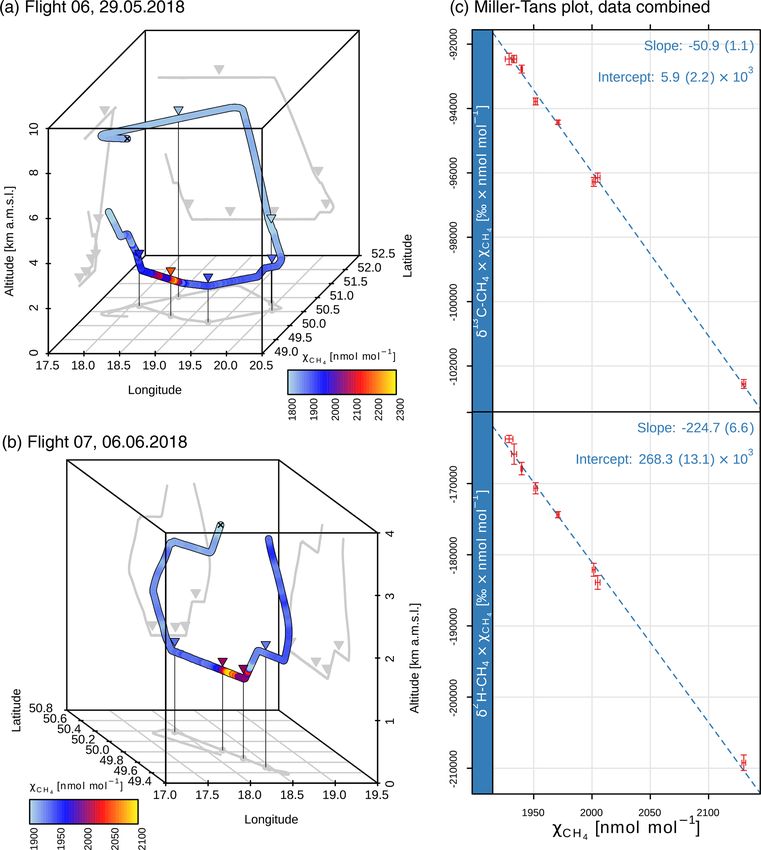
collected aboard the same platform. A careful in-flight cali- we were able to use the Miller–Tans approach to derive the
bration strategy together with post-flight quality assessment isotopic signature of the measured source, with values of δ 2 H
made it possible to determine both the single-measurement equal to −224.7 (6.6) ‰ and δ 13 C to −50.9 (1.1) ‰, giving
precision as well as biases against respective World Meteo- significantly lower δ 2 H values compared to previous studies
rological Organization (WMO) scales. We compare the re- in the area.
sult of greenhouse gas observations against two of the avail-
able global modelling systems, namely Jena CarboScope and
CAMS (Copernicus Atmosphere Monitoring Service). We
find overall good agreement between the global models and 1 Introduction
the observed mole fractions in the free tropospheric range,
characterised by very low bias values for the CAMS CH4 Increased mole fractions of atmospheric greenhouse gases
and the CarboScope CO2 products, with a mean free tropo- (GHGs) are recognised as the primary cause of the warm-
spheric offset of 0 (14) nmol mol−1 and 0.8 (1.3) µmol mol−1 ing observed in the climate system over the past 70 years.
Of these, the most important are carbon dioxide (CO2 ) and
Published by Copernicus Publications on behalf of the European Geosciences Union.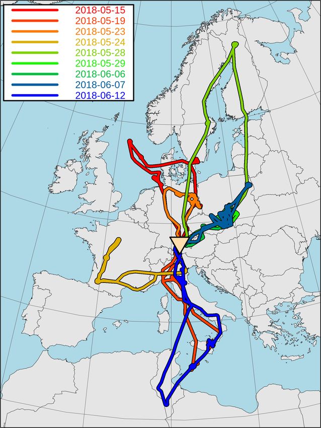
1526                                                   M. Gałkowski et al.: CoMet in situ observations of GHGs over Europe

methane (CH4 ), respectively responsible for approximately          mole fractions for atmospheric carbon dioxide (XCO2 ) and
56 % and 32 % of the globally averaged increase in radia-           methane (XCH4 ) come most often from surface-reflected
tive forcing caused by greenhouse gases, as compared to the         near-infrared and short-wave infrared radiation detectors
pre-industrial period (IPCC et al., 2013). Further increases        (Bovensmann et al., 1999; Kuze et al., 2009; Reuter et al.,
in the atmospheric burden of greenhouse gases are expected          2011; Butz et al., 2012; Eldering et al., 2012; Reuter et al.,
to lead to a multitude of negative impacts over a wide range        2019). While important insights into greenhouse gas bud-
of climate system components throughout the 21st century            gets have been gained (Bergamaschi et al., 2013; Basu et al.,
and beyond. These include further temperature increase, sea         2013), there are still significant limitations when using in-
level rise, changes in precipitation patterns, shrinking of ice     frared methods (Kirschke et al., 2013; Le Quéré et al.,
cover and more. Furthermore, cumulative emissions of CO2            2018). As an alternative to passive remote sensing, the in-
will have lasting effects on most aspects of climate for many       tegrated path differential absorption (IPDA) technique has
centuries, even if anthropogenic emissions are stopped alto-        been adapted in recent years to provide column-averaged
gether (IPCC et al., 2013).                                         measurements of greenhouse gas mole fractions with high
   The accuracy of climate projections is substantially re-         accuracy (e.g. Amediek et al., 2008; Sakaizawa et al., 2009;
duced, however, by uncertainties in the specific components         Spiers et al., 2011; Dobler et al., 2013; Du et al., 2017; Ame-
of greenhouse gas budgets, which stem either from diffi-            diek et al., 2017). All of these remote sensing techniques rely
culties in precise estimation of direct sinks and emissions         heavily on the availability of independent calibration and val-
or from our limited understanding of specific feedback pro-         idation data sets. A good overview on how remote sensing
cesses. Despite the critical importance of this issue, our          observations can be used to infer fluxes is presented in Varon
knowledge about even the two most important anthropogeni-           et al. (2018).
cally influenced greenhouse gases, CO2 and CH4 , is still in-          Aircraft measurements are flexible and constitute a critical
adequate. In fact, even though intense scientific and polit-        link for bridging the gap between ground-based networks and
ical activities have targeted this area of research over the        space-borne observations in constraining emissions at mul-
past 20 years, the uncertainties related to the most impor-         tiple scales. They can be performed either with precise in
tant source and sink processes remain high (Ballantyne et al.,      situ measurement techniques that can be calibrated and made
2015), reflecting the enormous complexity of the Earth sys-         traceable to World Meteorological Organization (WMO) cal-
tem, with its multitude of elements and feedback mecha-             ibration scales (e.g., Wofsy, 2011; Sweeney et al., 2015;
nisms, operating on a vast range of spatial and temporal            Filges et al., 2018; Boschetti et al., 2018; Umezawa et al.,
scales.                                                             2018) or utilising remote sensing instruments (Krings et al.,
   Main sources of uncertainties in the reported budgets are        2013). Airborne observations can be applied to describe re-
similar for both CO2 and CH4 . When considering bottom-             gional and local variability of the observed signals (Wofsy,
up methods, they are related either to (a) the lack of rep-         2011; Sweeney et al., 2015). They can also be used as vali-
resentativeness of flux measurement sites used for upscal-          dation of the coupled transport–emission models (Ahmadov
ing the fluxes from specific source areas or (b) incomplete         et al., 2007; Sarrat et al., 2007; Park et al., 2018; Leifer
knowledge at the process level, which affects the emission          et al., 2018) or used to directly infer the fluxes of measured
models used for the calculation of either emission factors or       components. Such direct inference has been demonstrated in
actual fluxes. Top-down methods, in turn, are based on in-          the past, e.g. using Gaussian plume models (Krings et al.,
verse modelling and critically depend on the availability of        2013), Lagrangian mass-balance approaches (Karion et al.,
high-precision atmospheric observations in the areas studied,       2013a; Cambaliza et al., 2014) or regional Bayesian inverse-
which is still insufficient. In order to significantly reduce the   modelling systems (e.g., Saeki et al., 2013; Boschetti et al.,
global uncertainties in the budgets of greenhouse gases us-         2018).
ing ground-based instrumentation, a significant expansion of           In order to further push the limits and improve the ob-
the observation networks is required to provide precise re-         servation and modelling methods developed in the past, a
gional budgets for the most important source and sink ar-           multi-platform aircraft research mission was envisaged, de-
eas (Ciais et al., 2014). Observation networks of sufficient        signed, proposed and executed in collaboration between the
density are currently only available over Europe and parts of       German Aerospace Center (DLR), the Max Planck Institute
North America, where they have been used successfully to            for Biogeochemistry (MPI-BGC), the University of Bremen,
constrain anthropogenic and biogenic fluxes of greenhouse           the Free University of Berlin, AGH University of Science and
gases (e.g. Bergamaschi et al., 2018).                              Technology and other partners. CoMet 1.0 (Carbon Diox-
   Utilising space-borne observations can bridge the data           ide and Methane Mission; see the overview paper by Fix et
gap by providing high-resolution data on regional scales            al. (2021, this special issue), executed in May and June 2018,
across the globe, which has driven significant develop-             targeted hotspots of CO2 and CH4 emissions in Europe, with
ments in remote sensing techniques since the mid-1990s.             a strong focus on the Upper-Silesian Coal Basin in Poland,
Since the launch of SCIAMACHY in 2002, remote sens-                 one of the largest regional emitters of methane. The mission
ing data on global distributions of column-averaged dry-air         utilised a multitude of state-of-the art instruments applied on

Atmos. Meas. Tech., 14, 1525–1544, 2021                                              https://doi.org/10.5194/amt-14-1525-2021
M. Gałkowski et al.: CoMet in situ observations of GHGs over Europe                                                           1527

both airborne and ground based platforms, including active
lidar (CHARM-F; see Amediek et al., 2017), passive remote
sensing (MAMAP; see Gerilowski et al., 2011; Krings et al.,
2013), in situ measurements (CRDS, QCLS; see, for exam-
ple, Filges et al., 2018) and satellite observations. Wher-
ever possible, these were applied simultaneously in order to
(a) achieve high observation inter-comparability, (b) test the
limits of applied measurement techniques, (c) provide a rich
suite of observations to evaluate atmospheric transport mod-
els and (d) to estimate regional GHG emissions.
    Here we present the results of in situ observations of atmo-
spheric greenhouse gases and methane isotopic composition
obtained over nine research flights of the German research
aircraft HALO (High Altitude and LOng Range Research
Aircraft) during CoMet 1.0, with the use of two airborne in-
struments installed aboard the aircraft during the campaign:
(i) JIG (Jena Instrument for Greenhouse gas measurements),
a continuous analyser for measurements of CH4 , CO, CO2
and H2 O and (ii) JAS (Jena Air Sampler), which collected
discrete 1 L samples for subsequent laboratory analyses of
CH4 , CO2 , H2 , N2 O, SF6 , O2 /N2 , Ar/N2 , δ 13 C−CH4 and
δ 2 H−CH4 .

2     Methods

2.1     CoMet 1.0 flights

During the CoMet 1.0 mission, HALO performed nine re-              Figure 1. Geographical extent of HALO research flights during the
search flights, with more than 63 h of observations over con-      CoMet 1.0 mission.
tinental Europe and parts of northern Africa (Fig. 1), with
the base of operations located in Oberpfaffenhofen (Bavaria,
Germany, marked with a triangle in the figure). During the
                                                                   order to fulfil conditions necessary for long-term deployment
campaign, each flight aimed to reach several scientific goals
                                                                   in the scope of IAGOS ERI (In-service Aircraft for a Global
based on the synoptic meteorological conditions over se-
                                                                   Observing System – European Research Infrastructure). De-
lected target areas. These goals included, for example, com-
                                                                   tailed development of the instrument, with the description of
parisons between active remote sensing and in situ observa-
                                                                   its operational parameters, is described in Chen et al. (2010)
tions, co-located measurements at satellite overpass points,
                                                                   and Filges et al. (2015, 2018). Here, only the basic operation
comparisons against other airborne instruments and others.
                                                                   principle and main differences to the IAGOS setup are given.
For each of those, a specific measurement strategy was
                                                                      The core method of the measurement is wavelength-
adopted. Those relevant for the measurements discussed in
                                                                   scanning cavity ring-down spectroscopy (CRDS), whereby
this study are described in Sect. 2.3. A complete description
                                                                   an infrared-wavelength laser light is injected into a high-
of the CoMet 1.0 mission will be given in an overview pub-
                                                                   finesse optical cavity. In the first phase of the measurement,
lication by Fix et al. (2021, this special issue).
                                                                   the strength of the incident laser beam gradually increases
2.2     In situ instrumentation                                    over time thanks to the resonance effect in the optical cav-
                                                                   ity, which also allows for the enhancement of the effective
2.2.1    JIG – Jena Instrument for Greenhouse gas                  absorption length and thus increases the detector’s sensitiv-
         measurements                                              ity. After reaching the designated signal level, the laser is
                                                                   turned off and the ring-down phase of the measurement be-
In situ continuous airborne measurements of greenhouse             gins. The time constant of the resulting exponential decay
gases on board HALO have been carried out using JIG (Jena          (ring-down time) depends on the absorption coefficient of
Instrument for Greenhouse gas measurements; photo avail-           the measured compound for the laser wavelength, tuned so
able in the Supplement, Fig. S1). The core of the device is        that the scan along selected individual spectral lines of the
a modified commercial analyser G2401-m, developed by Pi-           measured molecules is possible. The measurement requires
carro Inc. (Santa Clara, CA, USA), which was redesigned in         the usage of calibration gases, as well as careful control over

https://doi.org/10.5194/amt-14-1525-2021                                             Atmos. Meas. Tech., 14, 1525–1544, 2021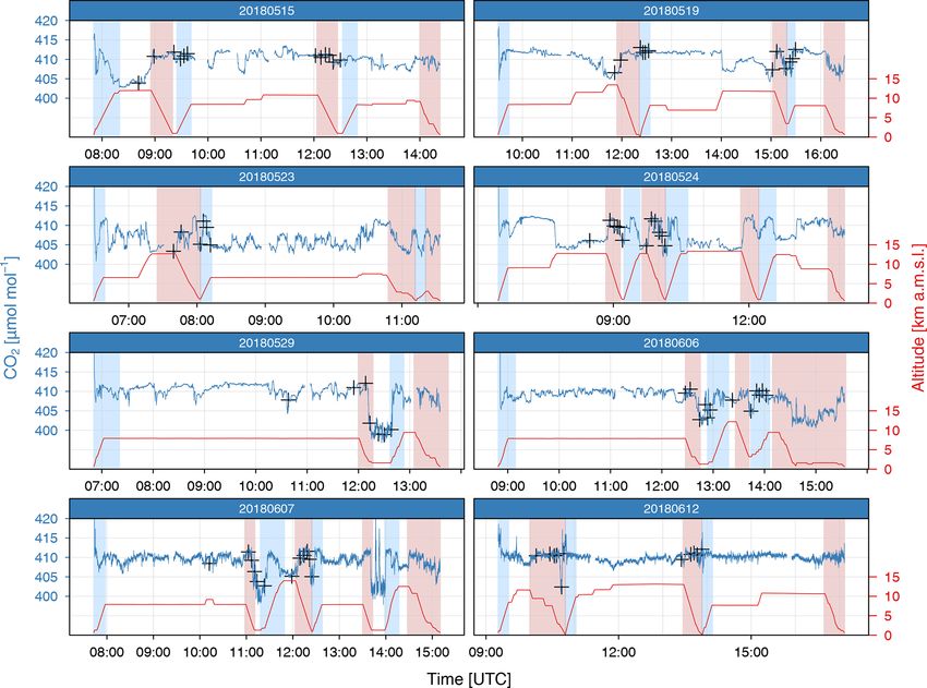
1528                                                M. Gałkowski et al.: CoMet in situ observations of GHGs over Europe

cavity pressure and temperatures in order to prevent sam-        clock reset) caused the loss of 96.8 % of in situ data from that
ple density variations. During the measurements described        day. The remaining 3.2 % have been excluded from the fol-
here, the cavity pressure was set at all times to 186.65 hPa     lowing analysis due to their fragmentation. The second mal-
(140 Torr) and the temperature to 45.00 ◦ C, with tolerance      function occurred during the power-up procedure on 7 June
levels of 0.13 hPa (0.1 Torr) and 0.02 ◦ C, respectively.        2018 (flight no. 8), when JIG suffered an unexpected shut-
   The instrument reports dry mole fractions, defined as the     down due to cabin overheating, which required a manual re-
number of molecules of each species in moles per one mole        set of a temperature switch. This in turn caused unintentional
of dry air, with typical observed ranges expressed in micro-     damage to the optical fibre mount located inside the instru-
moles per mole (µmol mol−1 ) for CO2 (equal to 1 part per        ment housing. The resulting loss of signal strength caused de-
million, ppm) and in nanomoles per mole (nmol mol− 1) for        terioration of the system parameters over flight nos. 8 and 9,
CO and CH4 (equal to 1 part per billion, ppb). As the col-       increasing noise and shifting the instrument calibration pa-
lected air was not dried in the sampling line, a water correc-   rameters. These were subsequently corrected using in-flight
tion was applied based on the online measurements of the         calibrations and post-mission laboratory calibrations. The
H2 O mole fraction, following the approach described in pre-     impact of the malfunction and final effect of applied correc-
vious studies of Filges et al. (2015) and Reum et al. (2019).    tions are discussed in Sect. 3.1.
   Calibration of the instrument was performed in the labo-
ratory before and after the CoMet 1.0 mission by measuring       2.2.2   JAS – Jena Air Sampler
three air mixtures, stored in working tanks, which covered
the range of ambient mole fractions of CO2 , CH4 and CO and      The sampler used during CoMet 1.0 (Fig. S1) is an airborne
had assignments traceable to the respective WMO calibration      version of the automated flask sampler developed within the
scales. All JIG trace gas mole fraction data provided in the     ICOS (Integrated Carbon Observing System) infrastructure.
current study are reported on the current WMO calibration        The device is equipped with 12 slots for holding 1 L glass
scales: CO2 X2007, CH4 X2004A and CO X2014A. The in-             flasks with automatically operated valves at both ends. Sam-
strument calibration was monitored during the mission with       ple air, collected outside the aircraft fuselage with a ded-
the use of two reference in-flight cylinders that contained      icated inlet, flows through tubing (PFA, 415 cm, 6.35 mm
dry mixtures of atmospheric air of known composition, for        (1/4 in.) OD) and into the drying unit (70 cm3 , stainless steel)
each tracer at a high and a low mole fraction, namely 373.4–     filled with magnesium perchlorate. The dryer is connected
397.4 µmol mol−1 for CO2 , 1661.0–1917.1 nmol mol−1 for          via another tubing section (PFA, 317 cm, 6.35 mm (1/4 in.)
CH4 and 77.4–139.5 nmol mol−1 for CO. These were anal-           OD, plus additional 15 cm of 6.35 mm (1/4 in.) OD, stain-
ysed several times during each flight. The calibration cycle     less steel, for pressure sensor mount) to a Teflon diaphragm
consisted of two intervals, each 3 min in length. The first      pump (N 813.3, KNF Neuberger GmbH) that provides the
minute of each interval was discarded in subsequent analyses     over-pressure necessary to flush and pressurise the flasks, up
due to pressure equilibration effects within the regulators.     to approximately 1500 hPa. The pump is connected directly
   Except for a single calibration check performed prior to      to the main input manifold (passing through all three rack-
take-off during a power-up procedure, all the other calibra-     mounted sub-units) via another flexible tube (PFA, 156 cm,
tion check cycles were enabled manually by an onboard op-        6.35 mm (1/4 in.) OD). The input manifold can be connected
erator of the system, during transit phases of the flight, in    to the output line either via open flasks (one or more) or a
contrast to the regular IAGOS implementation (Filges et al.,     two-way bypass valve. Each flask has its own pair of auto-
2015, 2018). The in-flight calibration checks occurred at high   mated motors responsible for operating its input (upstream)
altitudes, where high gradients of GHGs were not expected        and output (downstream) valves. At the end of the sampler
and the loss of information could be minimised. The last cal-    flow line, a mass flow meter (MFM; model D6F-20A6-000,
ibration cycle was always performed immediately before the       Omron) is installed that integrates the total volume of air
final approach of the flight. It should be noted that the re-    flowing through an opened flask, which ensures that the flask
sults of the in-flight calibration checks were only used for     volume has been sufficiently flushed with the sampled air (at
assessing a potential drift in the instrument calibration fac-   least 6 L under normal conditions). At the outlet of the sys-
tors relative to the pre-mission (April 2018) and post-mission   tem, a pressure release valve is installed that maintains the
(November 2018) laboratory calibrations.                         pressure at 1.5 bar and prevents the backflow of the pres-
   Additional, independent verification of the measurement       surised cabin air into the sampler in case of power failure.
quality was carried out by comparison of the mole fractions      Three pressure sensors and three thermometers are also in-
from in situ measurements and those obtained from labora-        stalled to monitor the status of the system.
tory analyses of air samples collected by the JAS (Jena Air          The sampler was controlled via computer in the electronic
Sampler; see Sect. 2.2.2 and the discussion of the results in    control section using dedicated software. The procedure for
Sect. 3.1).                                                      flask flushing and filling was enabled manually by an oper-
   Two malfunctions of the JIG occurred during the CoMet         ator, either at predetermined flight altitudes (in the case of
1.0 mission. On 28 May (flight no. 5), a software issue (i.e.    measurements of vertical profiles) or locations (e.g. plume

Atmos. Meas. Tech., 14, 1525–1544, 2021                                           https://doi.org/10.5194/amt-14-1525-2021
M. Gałkowski et al.: CoMet in situ observations of GHGs over Europe                                                                                 1529

sampling). Each flask was flushed with 10 times its volume         Table 1. Average measurement uncertainties of the flasks collected
prior to closing the upstream and downstream valves. Typ-          during CoMet 1.0. All values given with coverage probability of
ically, flasks were filled during descending profiles but on       0.68. A correction factor based on Student’s t distribution was ap-
some occasions also during ascents. The variable ambient           plied to account for low population size, following the Guide to the
pressure caused the flask fill time to vary between 100 s at       Expression of Uncertainty in Measurement (JCGM, 2008).
high altitudes and 25 s close to the surface.
   In order to precisely establish spatio-temporal coordinates         Compound             Precision        Uncertainty of          Unit
                                                                                                                 scale link
from which the sample is collected, a flow model has been
used that takes into account (i) flow information from the             CO2 a                     0.065                   0.046       µmol mol−1
MFM, (ii) the volume of tubing elements such as the dryer              CH4 a                       1.3                    0.70       nmol mol−1
and tubing and (iii) the varying physical length of tubing be-         N2 Oa                      0.13                    0.12       nmol mol−1
tween the inlet and the flask inlet slots (ranging from 10.76          H2 a                       0.31                    0.28       nmol mol−1
to 15.58 m). For each collected sample, a temporal weighting           SF6 a                     0.044                   0.025       pmol mol−1
function was calculated that represents the collected air vol-         O2 /N2 b                    1.5                     1.6       per meg
ume, following the approach suggested by Chen et al. (2012).           Ar/N2 b                     4.5                     6.0       per meg
   All flasks collected aboard HALO during CoMet 1.0 were              δ 13 C−CH4 c              0.046                    0.12       ‰
analysed in the GasLab of the Max Planck Institute for                 δ 2 H−CH4 c                0.49                     1.4       ‰
Biogeochemistry (MPI-BGC) in Jena, Germany, to estab-                a Precision calculated as the standard error of the repeated flask measurements
lish mole fractions of trace gases (CO2 , CH4 , N2 O, H2 ,           (usually between 3 and 5). An average standard error for a complete set of
                                                                     flasks collected during CoMet 1.0 is given. Uncertainty of the scale link
SF6 ) based on their respective WMO scales. Gas chromato-            specified as the root of the sum of squared uncertainties of (i) specified CCL
graphic analysis of air in glass flasks is done with a gas chro-     (Central Calibration Laboratory)-scale transfer uncertainties, (ii) precision limit
                                                                     of individual laboratory standard calibration events, and (iii) response drifts
matographic system based on two gas chromatographs (GCs;             between successive calibration events. For H2 , scale transfer uncertainty is
6890A, Agilent Technologies) equipped with a flame ioni-             equal to zero by definition, as flasks were measured directly against the primary
                                                                     scale. This uncertainty estimate does not include the accuracy of the respective
sation detector and a nickel CO2 converter (FID) for CH4             WMO scale.
                                                                     b O /N and Ar/N measurements were done on the BGC-IsoLab local
and CO2 , an electron capture detector (ECD) for N2 O and                2 2              2
                                                                     realisation of the Scripps scale. Realisation is achieved through the regular
SF6 , a helium ionisation pulsed discharge detector (D-3-I-          measurements of in-house standards against independently calibrated tanks
HP, Valco Instruments Co. Inc.) for H2 and a HgO Reduction           from Scripps. Reproducibility estimate is given as the average of standard
                                                                     deviations calculated from measurements against in-house standards (IsoLab,
Gas Analyser (RGA3, Trace Analytical) for H2 and CO. Ad-             MPI-BGC, Jena) of three cylinders with air mixtures calibrated independently
ditional analyses of O2 /N2 , Ar/N2 and isotopic composition         at Scripps Institute for Oceanography (SIO), covering the O2 /N2 range of
                                                                     −262.2 to −807.6 per meg and Ar/N2 range of 136.5 to 167.1 per meg.
of methane (δ 13 C−CH4 and δ 2 H−CH4 ) were carried out in           c Only a single measurement of each sample was possible. Precision estimated
the IsoLab of MPI-BGC (Sperlich et al., 2016). The typical           using repeated working standard measurements performed in sequence with the
                                                                     sample (usually four or five per sample). Reproducibility defined according to
measurement precision of the laboratory analyses is given in         Sperlich et al. (2016).
Table 1.
   A significant (approximately 10 nmol mol − 1) bias in CO
mole fractions was observed when comparing in situ mea-
surements from JIG against gas flasks collected using JAS.         and (iii) low-altitude legs, performed to assess the enhance-
Control laboratory experiments run after the campaign have         ments of CO2 and CH4 downwind of their sources (plume
shown that this bias was a result of a growth in CO mole           chasing).
fractions in the period between sample collection and sub-
sequent laboratory analysis. This enhancement in the mole
fraction could be attributed to new valve sealing polymer but      2.3.1    Large-scale variability in upper troposphere and
could not be accurately corrected; therefore we have decided                lower stratosphere
to discard these results. Careful quality control and additional
tests did not show any sign of other gases being affected.         Due to the constraints related to using other instruments (the
                                                                   active lidar), a significant amount of flight time was spent
2.3   Flight patterns                                              flying level at altitudes higher than 4 km, in order to emu-
                                                                   late a flight path similar to that of a satellite system. Typi-
Depending on the scientific goals set out before each re-          cal variability of in situ greenhouse gas mole fraction was
search flight, different flight patterns were executed in or-      low in these cases and is usually considered to be caused by
der to obtain the most valuable data. The main strategies          the intermixing of air masses coming from different regional
adopted for the CoMet 1.0 mission were (i) long-range gradi-       source areas. In situ data obtained in this manner are well
ent observations, designed to maximise the number of obser-        suited for validation of global chemistry models. As an ex-
vations for active lidar measurements with CHARM-F op-             ample, in Sect. 3.2 we compared JIG observations against
erated on HALO; (ii) vertical profiles, aimed mainly at the        well established modelling products: CAMS greenhouse gas
intercomparison between the lidar and in situ observations;        forecasts. A detailed model description is given in Sect. 2.4.

https://doi.org/10.5194/amt-14-1525-2021                                                   Atmos. Meas. Tech., 14, 1525–1544, 2021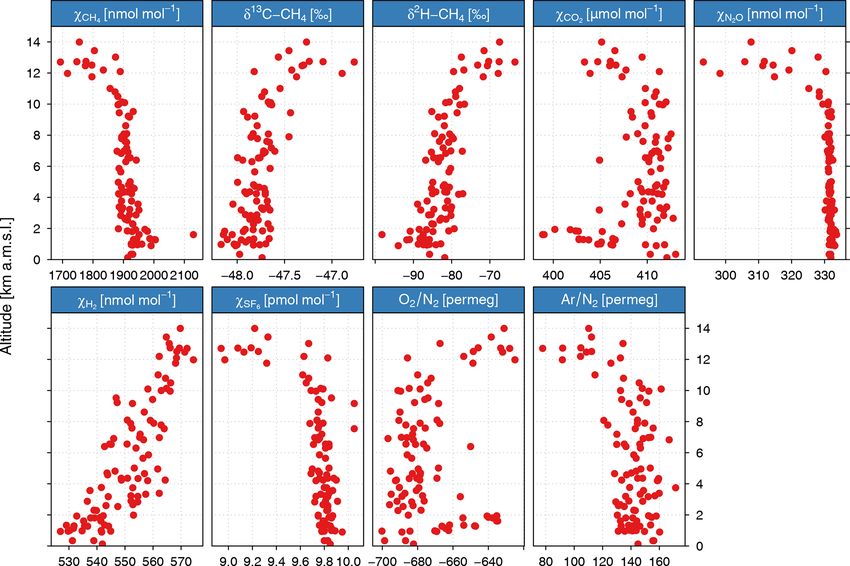
1530                                                  M. Gałkowski et al.: CoMet in situ observations of GHGs over Europe

2.3.2   Vertical profiles                                          where δobs is the measured isotopic signature, δbg is the back-
                                                                   ground signature, χobs is the mole fraction of the analysed
Multiple vertical profiles of the atmosphere were carried out      compound and χbg is the background mole fraction. Here,
during the campaign in order to establish the connection be-       similar to the Keeling approach, information on δ0 can be
tween column-integrated remote sensing and in situ measure-        gleaned from the application of linear regression; however
ments, thus also linking remote sensing observations to com-       the source signature is calculated from the slope, rather than
mon WMO scales for greenhouse gases. The typical strategy          intercept, of the linear fit formula. Following the study by
consisted of (i) a high-altitude overflight over a selected tar-   Cantrell (2008), we have applied a Williamson–York regres-
get, (ii) descent in the form of a spiral to the lowest possible   sion, which allows one to take into account uncorrelated er-
altitude above the target and (iii) subsequent ascent back to      rors in both the x and y axes of the data.
high altitude, usually flown along the shortest path in the di-       The Miller–Tans method relies on the appropriate assign-
rection of the next planned way-point.                             ment of the background signature (i.e. of the atmospheric
   Usually two or three vertical profiles were executed during     air outside of the plume). Long-term data available from at-
a given flight, depending on the availability of points of in-     mospheric observations show that the isotopic composition
terest and airspace accessibility. Wherever possible, profiles     of methane in the atmosphere is variable (Röckmann et al.,
were executed above (a) ICOS stations, (b) TCCON stations          2016; Nisbet et al., 2019) in both space and time. In order to
(Total Carbon Column Observing Network) and (c) Sentinel           estimate the background signature, we have used measure-
5P or GOSAT overpass locations. Flasks were also collected         ments from air samples collected in the immediate vicinity
during vertical soundings, at levels distributed between the       of the target plume, either from the upwind air masses or
minimum and maximum altitude, typically consisting of six          from outside of the main plume.
samples per profile (in some cases reduced to four).
   Measurements of vertical profiles are also of high interest
for model validation exercises, as the availability of highly      2.4   Models
precise data on greenhouse gases over Europe is currently
still limited. In the scope of the current study, we have as-      As part of the Copernicus Atmosphere Monitoring Service
sessed the performance of two well-established modelling           (CAMS), the European Centre for Medium-Range Weather
products (CAMS and Jena CarboScope; see Sect. 2.4) against         Forecasts (ECMWF) performs greenhouse gas simulations
CoMet 1.0 in situ observations.                                    based on its Integrated Forecasting System (IFS) and pro-
                                                                   vides operational global forecasting products focused on
2.3.3   Measurements in the planetary boundary layer –             greenhouse gases. In this work, we have used the 5 d high-
        plume chasing and isotopic composition                     resolution greenhouse gas forecast product from CAMS (ex-
                                                                   periment ID: gqpe, downloaded in April 2020; see Agusti-
A limited number of data were also collected inside the plan-      Panareda et al., 2017; Agustí-Panareda et al., 2019) in or-
etary boundary layer (PBL), usually during the lowest stage        der to validate the model using our observations. Further in
of vertical profile sounding. In several cases, however, these     the text, we will refer to these data as CAMS for simplic-
PBL sections were extended in order to cross low-level emis-       ity. Satellite data were used for initialisation of the forecast,
sion plumes (plume chasing). Of particular interest here are       namely TANSO-GOSAT for CO2 and CH4 and addition-
the flights over the Upper Silesian Coal Basin (a large re-        ally MetOp-IASI for CH4 (Massart et al., 2014, 2016). For
gional methane source) and downwind of the Bełchatów coal          CO, CAMS operational analysis (Inness et al., 2015, 2019)
power plant (the largest single emitter of CO2 in Europe, ac-      was used for forecast initialisation. Original CAMS 1 d fore-
cording to the European Pollutant Release and Transfer Reg-        cast data, available at the TCo1279 Gaussian cubic octahe-
ister, v16; E-PRTR, 2019). For both of these sources, clear        dral grid (equivalent to approximately 9 km horizontal reso-
enhancements from the strong sources were captured when            lution), were interpolated to 0.125◦ × 0.125◦ . The frequency
crossing the plume downwind.                                       of the analysed CAMS data was 3-hourly, and vertical reso-
   Additional to the in situ measurements, flasks were also        lution was the regular L137 ECMWF configuration.
collected to gather information about additional compounds            Additionally, CO2 data were also compared to the
and the stable isotopic composition of CH4 . For the cases         Jena CarboScope product (version s04oc_v4.3, Rödenbeck,
in which sufficient data were available, we have applied the       2005), further referred to as CarboScope. While the resolu-
method of Miller and Tans (2003), a variation of a classic         tion of the driving CarboScope model output fields is much
Keeling model (Keeling, 1958), in order to obtain the iso-         lower in this case (4◦ × 5◦ horizontal), the system benefits
topic mean source signature (δ0 ), expressed using relative        from using the fluxes of CO2 optimised using a Bayesian in-
delta notation. The method assumes a two-factor mixing of          version framework. A detailed description of the modelling
background air and methane-enhanced plume:                         system is given in Rödenbeck et al. (2003) and Rödenbeck
                                                                   (2005). The transport model TM3, which is used by Carbo-
δobs χobs = δ0 χobs − χbg (δbg − δ0 ),                      (1)    Scope, is described in Heimann and Körner (2003).

Atmos. Meas. Tech., 14, 1525–1544, 2021                                             https://doi.org/10.5194/amt-14-1525-2021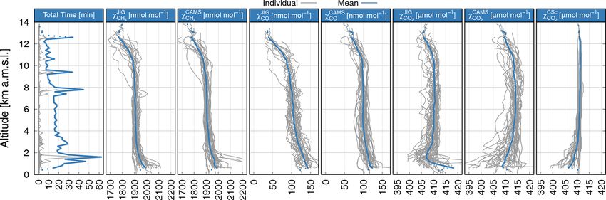
M. Gałkowski et al.: CoMet in situ observations of GHGs over Europe                                                                   1531

Figure 2. In situ mole fractions of CO2 measured throughout CoMet 1.0 with flight altitudes. Shading corresponds to the vertical profiles
discussed throughout the paper. Shading colours are denoted as follows: blue – ascending profile, red – descending profile. Co-located flask
measurements are marked with black crosses.

3     Results and discussion                                               Results from in-flight measurements of the two reference
                                                                        cylinders showed no significant drift; however the flight-
3.1    Overview and data quality                                        to-flight variation of each low- and high-span measurement
                                                                        during the period prior to the instrument malfunction on
A total of 55 h and 17 min of high-frequency (1 Hz) obser-              7 June was slightly larger than expected for CO2 : low-span
vations of CO2 , CH4 and CO were obtained aboard HALO                   measurements varied by 0.10 µmol mol−1 , 0.4 nmol mol−1
in the scope of the CoMet 1.0 campaign. Measurements                    and 1.0 nmol mol−1 , while high-span measurements varied
of CO2 are presented in Fig. 2, and a full overview, in-                by 0.14 µmol mol−1 , 0.3 nmol mol−1 and 0.8 nmol mol−1 for
cluding also CH4 and CO, is available in the Supplement                 CO2 , CH4 and CO, respectively. The likely cause for this is
(Fig. S2). Observations were performed at altitudes rang-               the silicon rubber membranes used in the pressure regulators
ing from approximately 50 m up to 14 km above mean sea                  (Filges et al., 2015), which are known to cause diffusion of
level. Data from 51 vertical profiles are available, of which           CO2 (Hughes and Jiang, 1995). Given that species other than
21 have simultaneous flask measurements. They are listed                CO2 did not show unexpected behaviour, we did not apply
in the Supplement (Table S1). A total of 15 in-flight cali-             any correction of the measurements resulting from the in-
brations were performed, making it possible for the single-             flight measurements of the reference cylinders. For this rea-
measurement precision to be estimated for flights no. 1–7.              son, we also did not apply any correction of drift within each
These were equal to 0.06 µmol mol−1 (CO2 ), 0.3 nmol mol−1              flight, in contrast to the experience of Karion et al. (2013b).
(CH4 ) and 3.1 nmol mol−1 (CO). Malfunction during the                     The comparison between flask and in situ measurements
roll-out procedure prior to flight no. 8 caused deterioration in        is available for all except one flight (no. 5). From the 96
the instrument noise for two subsequent flights (nos. 8 and             samples collected and analysed, 84 had simultaneous in situ
9), with values of precision increasing to 0.3 µmol mol−1 ,             measurements available from JIG that could be used for
1.5 nmol mol−1 and 50 nmol mol−1 for CO2 , CH4 and CO,                  a bias assessment. Here, we compare bias between both
respectively.                                                           our data sets to the “network compatibility goal”, defined

https://doi.org/10.5194/amt-14-1525-2021                                                   Atmos. Meas. Tech., 14, 1525–1544, 2021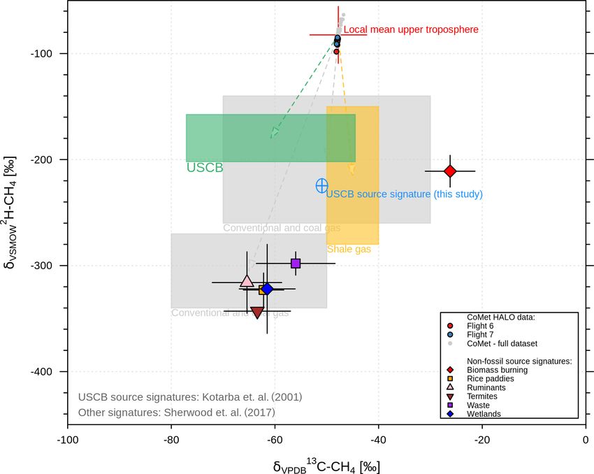
1532 M. Gałkowski et al.: CoMet in situ observations of GHGs over Europe
by the World Meteorological Organization as “the scien- ward flight over Italy, including a vertical profile in the vicin-
tifically determined maximum bias among monitoring pro- ity of Monte Cimone, with a subsequent crossing of Po Val-
grammes that can be included without significantly influenc- ley and the Alps, ending with landing at home base.
ing fluxes inferred from observations with models” (WMO, During the first section of the flight (Fig. 4, i), after the
2019). WMO specifies this compatibility goal as being equal initial climb, the aircraft stayed at high altitude (300 hPa,
to 0.1 µmol mol−1 for CO2 (in the Northern Hemisphere) and approximately 8 km a.m.s.l.), sounding the free troposphere
2 nmol mol−1 for both CH4 and CO. above the Po Valley. Comparison of measured concentra-
As shown in Fig. 3, the average bias for flights 1–7 tions to the model suggests that the chosen flight level
was equal to −0.131 (30) µmol mol−1 for CO2 and −2.93 was well within the free troposphere. Close to the surface,
(32) nmol mol−1 for CH4 , where numbers in parentheses CAMS predicted high enhancements of greenhouse gases,
represent standard uncertainty in the final digits quoted clearly visible on the CH4 and CO plots. At the time (10:00–
for the numerical value. Larger spread when independent 11:00 UTC), the boundary layer was still developing, reach-
measurements are considered (Fig. 2) stems mainly from ing only about the 900 hPa level (approximately 1000 m).
the imperfect match between the temporal coordinates of After crossing the coastline, the aircraft ascended to a
the two instruments, which can be considered random and cruise altitude of 250 hPa (approximately 12 km). Around
does not cause systematical shift. After the malfunction 11:30 UTC it reached the tropopause level and, after another
(see Sect. 2.2.1), i.e. for flights no. 8 and 9, these mean increase in altitude, entered into the stratosphere for approx-
offsets were equal to 0.127 (68) µmol mol−1 and −0.64 imately 10 min immediately prior to the vertical sounding
(91) nmol mol−1 for the respective gases. While the differ- at Lampedusa (Fig. 4, ii). The vertical structure of the at-
ence of values as compared to flights 1–7 is statistically sig- mosphere was generally well predicted in the model (see
nificant, it is still close to the WMO compatibility goal. Sect. 3.4 and also Figs. S3–S18), albeit larger differences can
be observed in the lowest 3 km of the profile, especially for
3.2 Large-scale variability CO2 .
The Mt. Etna section of the flight (Fig. 4, iii) took place
Out of the total number of observations during CoMet 1.0, mostly in the free troposphere, and no significant gradi-
84 % were performed at altitudes above 4 km and are of ents were observed for either of the measured compounds.
particular interest for model validation. To demonstrate the Subsequent transfer over southern Italy (iv) started with
utility of the observations to validate model results, as well an ascent into the stratosphere (at approximately 220 hPa,
as to help understand the patterns in measured mole frac- 13 km a.m.s.l.). After 10 min of northward flight, the aircraft
tions, we analyse and compare JIG measurements to CAMS crossed into the troposphere horizontally again.
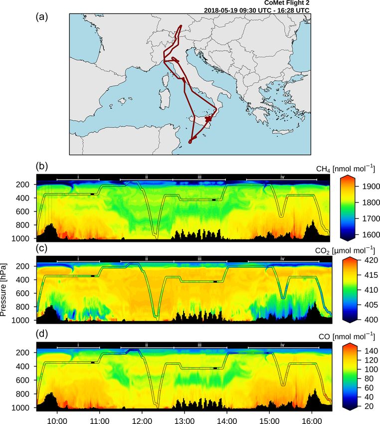
high-resolution products for CO2 , CH4 and CO. Flight no. 2 Immediately before the descent to Monte Cimone, it
(shown in light red in Fig. 1) is discussed as an example. crossed a stratospheric air filament, possibly brought down
The flight (Fig. 4a) was executed on 19 May 2018, with the to the flight level by the outflow of a deep convective sys-
main goal of capturing the large-scale variability of green- tem active in the area in the afternoon on that day. This is
house gases in the atmosphere above Italy and the Mediter- corroborated by CAMS model results, which show a clearly
ranean coast. Two vertical profiles were planned above ICOS defined air-mass structure, depleted in mole fractions for all
stations, namely Lampedusa (35◦ 310 0500 N, 12◦ 370 5000 E) and the observed compounds, stretching from the stratosphere
the Monte Cimone mountain station (Tuscan–Emilian Apen- at 200 hPa down to approximately 400 hPa (corresponding
nines; 44◦ 110 38000 N, 10◦ 420 05000 E). The latter profile was to roughly 13 and 8 km a.m.s.l., respectively). Shortly af-
executed approximately 20 km away from the target due to ter that, the aircraft descended, making a downward spiral
an active thunderstorm over the site. Other points of interest over the northern Apennines, down to approximately 700 hPa
were the Po Valley, crossed twice (morning and afternoon) (3.5 km). The model–observation discrepancy is much higher
at high altitude, and two high-altitude circles around Mount at this point, most probably due to (i) errors in representation
Etna (35◦ 310 05000 N, 12◦ 370 50000 E). of the local convective systems or (ii) errors in the surface
Figure 4b–d show the CAMS model results extracted at fluxes driving the modelled mole fractions or a mixture of
the geographical aircraft time and location, together with cor- both. The high-resolution CAMS product correctly captures
responding in situ observations from JIG overlaid on the air- most of the large-scale phenomena. There are, however, spe-
craft flight path, both plotted using the same colour scale. The cific situations in which the performance of the model drops,
model captures most of the features observed in the atmo- specifically in the vicinity of strong local convection systems,
sphere. Speaking in terms of observed spatial and temporal where parameterisations can sufficiently predict neither the
variability of the atmospheric composition (modelled and ob- height nor the transport of the strong enhancements present
served), four sections of the flight can be identified: (i) morn- in the Po Valley. The reasons behind this discrepancy may
ing overflight over northern Italy; (ii) passage over Mediter- stem from the inability of coarser scale parameterisations to
ranean Sea, ending with a vertical sounding at Lampedusa; capture local phenomena accurately or from an incorrect dis-
(iii) circling Mount Etna at medium altitude; and (iv) north- tribution of the ground-level sources.
Atmos. Meas. Tech., 14, 1525–1544, 2021 https://doi.org/10.5194/amt-14-1525-2021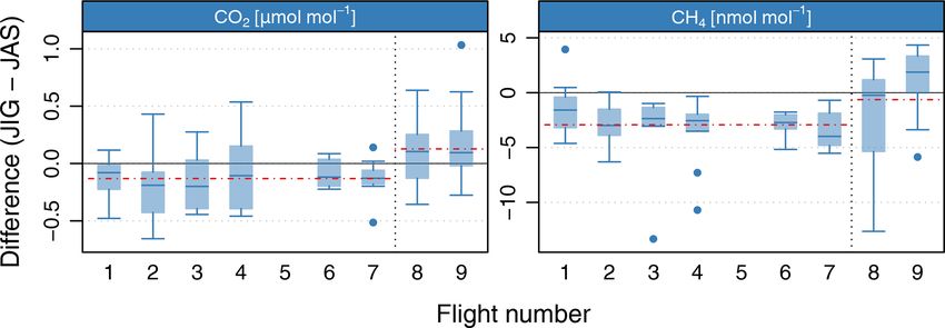
M. Gałkowski et al.: CoMet in situ observations of GHGs over Europe 1533
Figure 3. Comparison between JIG results and analysis of flasks collected during CoMet 1.0 aboard HALO. Data from the last two flights
(separated by the dashed line) indicate a residual change in calibration, following an instrument malfunction. See text for details.
In the following section, we analyse the model–data mis- On average we have observed a 4 µmol mol−1 decrease for
match more closely using the subset of CoMet 1.0 data col- CO2 between 10 and 13 km, which is most probably caused
lected only during the vertical soundings. by the increasing age of the slow-mixing stratospheric air
(Andrews et al., 2001). Decreases of CH4 and CO are more
3.3 Vertical structure of the atmosphere pronounced (on average 150 and 70 nmol mol−1 , i.e. 8 % and
45 % relative to the value at 10 km), underlining an increased
All profiles of CO2 , CH4 and CO collected with JIG are oxidative breakdown of these tracers (added to the age effect
presented in Fig. 5, together with comparison to the Carbo- in case of CH4 ).
Scope and CAMS model products. Individual comparisons While the observed gradient is similar to previously re-
are available in the Supplement (Figs. S3–S10 and S11–S18). ported studies (e.g. Wofsy, 2011; Sweeney et al., 2015;
It should be noted that the mean profile for the lowest alti- Umezawa et al., 2018), measurements from CoMet 1.0 also
tudes is dominated by a limited number of cases when the clearly indicate the increase in atmospheric concentrations
ground level was reached. This happened most often at home over the past years. For example, the CH4 mole fractions
base (EDMO, Oberpfaffenhofen). Similarly, only a limited measured during the IMECC campaign in autumn 2009
number of profiles reached altitudes beyond 12 km a.m.s.l. (Geibel et al., 2012) were approximately 60 nmol mol−1
Again, three distinct altitude ranges can be distinguished lower throughout the atmospheric column than those ob-
based on the observed gas mole fractions and their vari- served in 2018. This number is closely in line with the mean
ance. The lowest, the PBL, is characterised by highly vari- global atmospheric growth of methane of 63.8 nmol mol−1
able concentrations and is located in the altitude range of (between 2009 and 2018; NOAA, 2020).
0–3 km. Both the highest and lowest observed concentra-
tions of CO2 were observed here, with most of the obser- 3.4 Model validation
vations in the range between 400 and 420 µmol mol−1 . Occa-
sionally, peaks of over 420 µmol mol−1 were observed in the The vertical profile subset of the measurements was the basis
vicinity of strong point sources (e.g. Bełchatów power plant). of the comparison to the well-established global modelling
CH4 and CO variability were also high, with most observed systems CAMS and CarboScope. Here, we focus on describ-
values between approximately 1880 and 2000 nmol mol−1 ing the vertical structure of the model–data mismatch, de-
for methane (with peaks above 2100 nmol mol−1 ) and 100– fined as the difference between the modelled results and in
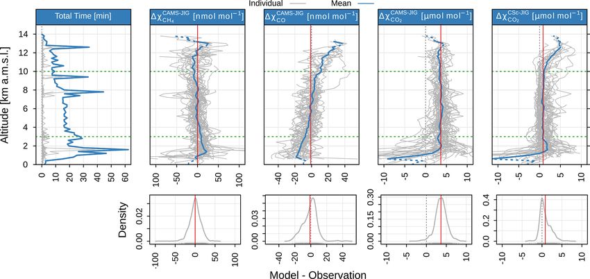
150 nmol mol−1 for carbon monoxide. situ observations from JIG, presented in Fig. 6. Mirroring
Above the PBL range, free tropospheric observations were previous discussion of different characteristics of the atmo-
characterised by much smaller variability. For CO2 , the mean sphere, here the different nature of discrepancies can also
profile becomes flat, with a value of 410 µmol mol−1 up to be separated into three distinct layers of the atmosphere. It
approximately 10 km altitude. For CH4 and CO, a vertical is worth noting that the model–observation mismatch is, in
gradient in the mean values is observed, reflecting the bal- general, constant in neither space nor time, as can be seen
ance between surface anthropogenic sources, large-scale ad- when analysing the variability between different flight days.
vection and tropospheric chemical sinks. However, some important conclusions can be drawn when
Above the altitude of 10 km, a more pronounced decrease analysing the overall vertical structure in the difference be-
in the mole fractions is observed, which is directly related to tween global model results and CoMet 1.0 in situ observa-
occasional crossings into the tropopause region and the low- tions.
ermost stratosphere. The variability of the observed decrease The variability in the mismatch is highest closest to the
is large and follows the variability in the tropopause height. surface (bottom 3 km), which is related to influences from
https://doi.org/10.5194/amt-14-1525-2021 Atmos. Meas. Tech., 14, 1525–1544, 20211534 M. Gałkowski et al.: CoMet in situ observations of GHGs over Europe Figure 4. Curtain plot showing results for 19 May 2018. (a) Overview map with flight path. Time series of aircraft altitude, with CAMS model results as colour plot in background for (b) CH4 , (c) CO2 and (d) CO; coloured lines superimposed on the curtain plot denote in situ measurements from HALO, with mole fractions plotted in the same colour scale. Ranges labelled (i) to (iv) within the panels denote distinct sections of the flight as follows: (i) initial southward crossing of the Po Valley, (ii) passage over Mediterranean towards Lampedusa ending with a vertical sounding near the ICOS station, (iii) circular flights over Mt. Etna, (iv) northward flight over northern Italy with a profile attempted over Mt. Cimone. See the discussion in the text for details. local sources and sinks as well as variability of atmospheric sult of its low spatial resolution. As the in situ measurements mixing and transport in the PBL, which are hard to represent from CoMet 1.0 are not numerous enough to give a robust es- at respective model resolutions (0.125◦ × 0.125◦ for CAMS, timate for the European region, and differences between the 4◦ × 5◦ for CarboScope). Another source of mismatch is re- model predictions and observations will be heavily depen- lated to uncertainties in the emissions data used by the mod- dent on a specific synoptic range and distribution of sources els. Validation of individual emission sources, while of criti- in the vicinity, we do not provide any general statistics for cal importance, remains challenging. In addition, in the case this lowest part of the atmosphere. of biospheric CO2 , the prediction of fluxes on scales relevant In the free tropospheric range, the mismatch represents the for direct comparison of mole fractions on regional scales large-scale offset between the model and observations bet- also remains a difficult task. This is true for all the analysed ter and is only weakly dependent on the spatial distribution compounds and both models, with a markedly larger discrep- of the emissions sources. Under this assumption, the mis- ancy in the CarboScope product that clearly suffers as a re- match is mostly caused either by (i) large-scale (i.e. at least Atmos. Meas. Tech., 14, 1525–1544, 2021 https://doi.org/10.5194/amt-14-1525-2021
M. Gałkowski et al.: CoMet in situ observations of GHGs over Europe                                                                          1535

Figure 5. An overview of the vertical profiles measured during the CoMet 1.0 mission, together with modelled profiles from CAMS and
CarboScope (denoted with CSc). In the first panel, total time is calculated as a sum of 1 s observations from each respective bin. All the other
panels present mole fractions for different variables, binned into 200 m layers. Averages for each layer are shown as a solid blue line, while
solid grey lines represent individual profiles. Dashed lines represent the means with less than 200 s of observations available. Only data from
the individual profiles marked on Fig. 2 are plotted here; i.e. the measurements collected during horizontal sections of the flights are not
included.

Figure 6. Top row: the first panel shows time spent in each altitude bin (200 m) for individual flights (grey lines) and the sum for CoMet 1.0
(solid blue). The four panels to the right show differences between modelled (CAMS and CarboScope, latter abbreviated as CSc) and mea-
sured mole fractions as a function of altitude (grey – individual flights, blue – average per altitude bin). Dashed red line represents the average
value in the altitude range 3–10 km (vertical range marked with horizontal dashed green lines). Bottom: density plots for measurements in
the free tropospheric (3–10 km) range.

national) offsets in emission strengths; (ii) bias in the initial-          with height for CH4 and CO2 , with a symmetric distribu-
isation of the forecasted fields (with CAMS GHG and op-                     tion around a mean value (CH4 : 0 (14) nmol mol−1 ; CO2 :
erational analysis fields which are a combination of model                  3.7 (1.5) µmol mol−1 , where standard uncertainty in the fi-
simulation and satellite observations); or (iii) errors in chem-            nal digits is given in brackets. For CO2 , a substantial offset
istry parameterisations (OH radical reaction chains, CH4 and                is still present, most probably connected with errors in the
CO).                                                                        strength of the net biospheric fluxes predicted in the model.
   In the CAMS product, the offset between the modelled                     This general offset needs to be taken into account if the data
values and observations in the troposphere becomes stable                   are either compared directly to the measurements (this paper)

https://doi.org/10.5194/amt-14-1525-2021                                                        Atmos. Meas. Tech., 14, 1525–1544, 2021
1536                                                M. Gałkowski et al.: CoMet in situ observations of GHGs over Europe

or used as lateral boundary conditions for regional modelling    validation, important constituents were monitored, offering
studies. For CO, a sloped model–data mismatch is observed,       further insights into the state of the atmosphere over Europe
most likely related to known issues with the inventories of      during the CoMet 1.0 mission. The general nature of the col-
anthropogenic emissions of CO (e.g. Boschetti et al., 2015)      lected data follows the patterns described for in situ data,
superimposed on chemistry-related effects. The mean value        with three distinct abundance regimes: (i) PBL, (ii) residual
of the offset of CO in the 3–10 km altitude range is equal to    layer/free troposphere and (iii) tropopause and lower strato-
−1.0 (8.8) nmol mol−1 .                                          sphere, however with some marked differences.
   For altitudes above 10 km, the mismatch between CAMS             For N2 O and SF6 , both potent greenhouse gases (IPCC
and observations shows larger variability for CH4 and CO,        et al., 2013), there is no clearly visible mole fraction gra-
with CO2 discrepancies similar to those observed in the          dient between the PBL and the free troposphere. For both
free troposphere. While the number of observations at these      gases, the variability is known to be dominated by the slow
higher altitudes is relatively low compared to those below       stratospheric transport, effectively causing the “age” of air
10 km, we believe that these differences are also caused by      masses to be higher than the tropospheric air below (An-
errors in both transport and chemistry schemes in the IFS        drews et al., 2001). For N2 O, this effect is superimposed on
system. These have been investigated in some detail in the       the additional signal caused by its photochemical destruc-
case of CH4 , for which the errors in the stratosphere have      tion in the stratosphere. Notably, during CoMet 1.0, two sam-
been found to be larger than those observed in the tropo-        ples were collected with SF6 mole fractions elevated by ap-
sphere (Verma et al., 2017).                                     proximately 0.2 pmol mol−1 . The first was filled on 7 June,
   Optimised CO2 mole fractions from CarboScope also             at 9.2 km altitude, over Czechia, and second on 12 June, at
show overall good agreement when compared to observa-            7.6 km, during the downward profile over the Po Valley. The
tions, despite lower model resolution compared to CAMS.          potential source of these two observations might be worth
The model–data mismatch is dominated by a random term            investigating, especially in light of the constant atmospheric
in the free tropospheric range (0.8 (1.3) µmol mol−1 ). In-      increase of the SF6 , despite substantial efforts to curb emis-
terestingly, the distribution of the mismatch in this altitude   sions of this potent greenhouse gas (Weiss and Prinn, 2011).
range is a positively skewed Gaussian curve (Fig. 6, bottom-     Some attention was also given to molecular hydrogen (H2 )
right panel), with the values in the main peak almost sym-       due to its potential feedbacks to the atmosphere oxidative ca-
metric around 0 µmol mol−1 and the mean offset in the 3–         pacity and stratospheric ozone levels (see Batenburg et al.,
10 km range driven by the values in the tail of the distribu-    2012, and references therein). Values measured during the
tion. The most probable cause is the inability of the model      mission, namely 540 nmol mol−1 near the surface, approxi-
to represent convective uplifting of CO2 -depleted air from      mately 550–560 nmol mol−1 throughout the free troposphere
the PBL. It should also be noted that in the CarboScope          and approximately 570 nmol mol−1 in the lower stratosphere,
product, a systematic over-prediction of CO2 mole fractions      are comparable to previously reported values, e.g. in the
above 10 km (up to 5 µmol mol−1 ) is observed, which might       scope of the CARIBIC project (Batenburg et al., 2012). This
be caused either by (i) significant errors in the tropopause     structure is driven by the presence of a relatively strong soil
height or (ii) vertical mixing in the lower stratosphere that    sink in the latitude band covered during CoMet 1.0, as has
is too fast, leading to underestimation of the gradient and      been confirmed by modelling studies (e.g. Pieterse et al.,
the chemical age of CO2 . In the PBL range, the mole frac-       2011). O2 /N2 and Ar/N2 ratios are presented for complete-
tions are generally underestimated, sometimes by more than       ness but are not discussed in the present study.
10 µmol mol−1 , albeit such a large discrepancy is only visi-       Of particular interest during CoMet 1.0 was the sta-
ble for the lowest altitude range (less than 1 km), where the    ble isotopic composition of methane. Abundances of both
sample size is low. Where the observation set is more ro-        δ 13 C−CH4 and δ 2 H−CH4 are strongly and negatively cor-
bust, the bulk of observations is characterised by differences   related (R = −0.88 and R = −0.96, respectively) with mole
smaller than 10 µmol mol−1 and can have either positive or       fractions of methane, signifying the potential to use the iso-
negative sign. Such behaviour is to be expected when trying      topes as a marker of the source processes. Indeed, in the next
to compare local plume enhancements to the low-resolution        section we present an application of using isotopic compo-
model results that averages over large, inhomogeneous areas      sition to differentiate between specific source types in the
characterised by a dynamic spatio-temporal diurnal cycle of      study area of the Upper Silesian Coal Basin (USCB, southern
fluxes.                                                          Poland).

3.5    Additional data from discrete samples – JAS               3.6   Capturing the USCB source signature with isotopic
                                                                       data
Figure 7 presents additional data acquired throughout the
campaign with discrete samples, with a detailed overview         Due to the broader spatial range covered by the HALO air-
provided in the Supplement (Fig. S19 and Table S1). Apart        craft, the number of samples taken over the USCB area using
from CH4 and CO2 , for which the flask data were used for        the JAS instrument was limited to 12 flasks, collected over

Atmos. Meas. Tech., 14, 1525–1544, 2021                                           https://doi.org/10.5194/amt-14-1525-2021
You can also read