Retracing hypoxia in Eckernförde Bight (Baltic Sea)
←
→
Page content transcription
If your browser does not render page correctly, please read the page content below
Biogeosciences, 18, 4243–4264, 2021
https://doi.org/10.5194/bg-18-4243-2021
© Author(s) 2021. This work is distributed under
the Creative Commons Attribution 4.0 License.

Retracing hypoxia in Eckernförde Bight (Baltic Sea)
Heiner Dietze and Ulrike Löptien
Institut für Geowissenschaften, CAU Kiel, Ludewig-Meyn-Str. 10, 24118 Kiel, Germany

Correspondence: Ulrike Löptien (ulrike.loeptien@ifg.uni-kiel.de)

Received: 8 February 2021 – Discussion started: 12 February 2021
Revised: 27 May 2021 – Accepted: 22 June 2021 – Published: 20 July 2021

Abstract. An increasing number of dead zoning (hypoxia)           ber – and (2) the local ventilation of bottom waters by local
has been reported as a consequence of declining levels of dis-    (within EB) subduction and vertical mixing. Biogeochem-
solved oxygen in coastal oceans all over the globe. Despite       ical processes that consume oxygen locally are apparently
substantial efforts a quantitative description of hypoxia up to   of minor importance for the development of hypoxic events.
a level enabling reliable predictions has not been achieved       Reverse reasoning suggests that subduction and mixing pro-
yet for most regions of societal interest. This does also apply   cesses in EB contribute, under certain environmental condi-
to Eckernförde Bight (EB) situated in the Baltic Sea, Ger-        tions, to the ventilation of the KB by exporting recently ven-
many. The aim of this study is to dissect underlying mech-        tilated waters enriched in oxygen. A detailed analysis of the
anisms of hypoxia in EB, to identify key sources of uncer-        2017 fish-kill incident highlights the interplay between west-
tainties, and to explore the potential of existing monitoring     erly winds importing hypoxia from KB and ventilating east-
programs to predict hypoxia by developing and documenting         erly winds which subduct oxygenated water.
a workflow that may be applicable to other regions facing
similar challenges. Our main tool is an ultra-high spatially
resolved general ocean circulation model based on a code
framework of proven versatility in that it has been applied       1   Introduction
to various regional and even global simulations in the past.
Our model configuration features a spacial horizontal reso-       The impact of humans on the Earth system has reached a
lution of 100 m (unprecedented in the underlying framework        level of magnitude comparable to natural influences. Among
which is used in both global and regional applications) and       the changes apparently accompanying our way into the
includes an elementary representation of the biogeochemical       Anthropocene are decreasing oxygen concentrations in the
dynamics of dissolved oxygen. In addition, we integrate ar-       global oceans. This decrease in oxygen is manifesting itself
tificial “clocks” that measure the residence time of the water    most prominently in coastal regions: in the 1960s only 42 of
in EB along with timescales of (surface) ventilation. Our ap-     the so-called “dead zones”, which no longer permit the sur-
proach relies on an ensemble of hindcast model simulations,       vival of higher animals, were reported. In 2008 this number
covering the period from 2000 to 2018, designed to cover a        already increased to 400 (Diaz and Rosenberg, 2008). The
range of poorly known model parameters for vertical back-         implications can be substantial, including mass mortality of
ground mixing (diffusivity) and local oxygen consumption          (commercial) fish, loss of blue carbon (associated with sea-
within EB. Feed-forward artificial neural networks are used       grass habitat loss), degradation of touristic and recreational
to identify predictors of hypoxia deep in EB based on data at     assets, and release of the potent greenhouse gas N2 O (e.g.,
a monitoring site at the entrance of EB.                          Naqvi et al., 2010).
    Our results consistently show that the dynamics of low           The Baltic Sea in central northern Europe is a prominent
(hypoxic) oxygen concentrations in bottom waters deep in-         example of a coastal region that has been exposed to inter-
side EB is, to first order, determined by the following an-       mittent dead zoning (i.e., hypoxic events) in the past (Zillén
tagonistic processes: (1) the inflow of low-oxygenated water      et al., 2008). Apparently hypoxia has increased over time in
from the Kiel Bight (KB) – especially from July to Octo-          response to anthropogenic nutrient inputs and ocean warm-
                                                                  ing (Jonsson et al., 1990; Carstensen et al., 2014). Conse-

Published by Copernicus Publications on behalf of the European Geosciences Union.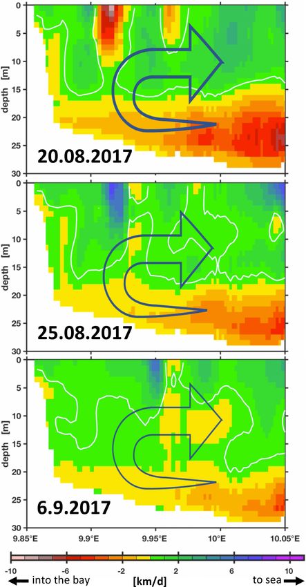
4244                                                       H. Dietze and U. Löptien: Retracing hypoxia in Eckernförde Bight

quently, international mitigation measures are put into action
by the highly industrialized and populated bordering nations
(e.g., Helsinki Convention, EU Marine Strategy Framework
Directive, Baltic Sea Action Plan), and a discussion of geo-
engineering options targeted at containing dead zoning has
been opened (Stigebrandt and Kalen, 2013; Stigebrandt et al.,
2015; Liu et al., 2020).
   The mechanisms behind the dynamics of oxygen dissolved
in seawater are well known: oxygen is produced as a by-
product of organic matter production by autotrophs in the
sunlit surface ocean. Organic matter is exported to depth
where its remineralization is typically associated with oxy-
gen consumption by bacteria. Air–sea fluxes of oxygen may
be in- or outgoing depending on whether the ocean’s surface
is over- or undersaturated. Typical surface concentrations of
dissolved oxygen are around a few hundred millimoles O2
per cubic meter (mmol O2 m−3 ), predominantly set by physi-
cal solubility as a function of temperature and salinity. Addi-
tional complexity is added by the ocean circulation which de-
termines the timescales on which oxygen sources and sinks           Figure 1. Overview map. The colors indicate water depth (in m).
may accumulate before antagonistic processes set in. This
holds especially for the Baltic Sea where sporadic inflows
of salty and oxygenated North Sea surface waters replace            the longest-operated time series stations worldwide (e.g.,
oxygen-deprived bottom waters of the Baltic Sea (Matthäus,          Lennartz et al., 2014). Consequently, EB is exceptionally
2006) and where wind-driven upwelling has been identified           well sampled, which facilitates the development of numer-
as a key process effecting vertical exchange of heat and nu-        ical models and piloting approaches which may be put to
trients (e.g., Lehmann and Myrberg, 2008).                          use in other coastal regions threatened by hypoxia (such as
   Even though there is consensus regarding the underlying          other Baltic Sea regions, the East China Sea, and Cheasa-
processes, the numerical quantitative simulation of hypoxic         peake Bay). The overarching aim is to “. . . identify critical
conditions remains challenging because it is, essentially, the      processes. . . ” and to “. . . provide a supreme dynamic test of
quest to simulate extreme (low) values that are determined by       knowledge. . . ” (Flynn, 2005) by simulating hypoxia in EB
the difference of relatively large and uncertain numbers. This      using a code framework that is proven to be easily applica-
introduces high uncertainty to both the open ocean model ap-        ble globally (e.g., in Dietze et al., 2017), near-globally (e.g.,
plications (e.g., Cocco et al., 2013; Dietze and Löptien, 2013;     in Dietze et al., 2020), and regionally (e.g., in Dietze et al.,
Löptien and Dietze, 2017) and Baltic Sea model applications         2014). We use an ensemble approach of a suite of regional
(Meier et al., 2011, 2012), which limits their contribution         coupled biogeochemical ocean models targeted at dissecting
to management or geoengineering decisions of stakeholders.          uncertainties of the biogeochemical module from those of the
For example, it has been illustrated in a global model that         ocean circulation module. The analyses are aided by integrat-
deficiencies in biogeochemical model components may be              ing artificial tracers measuring residence times – a concept
compensated for by deficiencies in circulation model compo-         essential to understanding hypoxia (e.g., Fennel and Testa,
nents (Löptien and Dietze, 2019), thereby obscuring even the        2019). Finally, we use an artificial neuronal network (ANN)
sign of the sensitivity of the (global) warming to come. This       to identify the critical processes that make the oxygen defi-
raises the question if it is actually feasible to reliably (i.e.,   ciency deep in the EB predictable – an approach which also
getting the right answer for the right reason) simulate low-        gives guidance on the question of where uncertainty may
oxygen events in systems such as the Baltic Sea that are (1)        lurk.
infamous for their natural variability (Meier et al., 2021) and
(2) subject to antagonistic effects of improved management
of water resources and climate change on oxygen concentra-          2   Methods
tions (e.g., Lennartz et al., 2014; Hoppe et al., 2013), which
is notoriously difficult to deconvolve (Naqvi et al., 2010).        MOMBE (Modular Ocean Model Bight of Eckernförde) is
   The present study steps forward to simulate oxygen dy-           a new configuration of a general ocean circulation model
namics at the exemplary site Eckernförde Bight (EB) which           (GCM). The GCM is coupled to a simple representation of
is an appendix to the Kiel Bight (KB) in the German part            biogeochemical processes by introducing an additional pas-
of the Baltic Sea (Fig. 1). The EB site is special in that          sive tracer that is advected and mixed just like the tracer
it hosts the monitoring station Boknis Eck (Fig. 2), one of         temperature and salinity but, other than that, is controlled by

Biogeosciences, 18, 4243–4264, 2021                                                    https://doi.org/10.5194/bg-18-4243-2021
H. Dietze and U. Löptien: Retracing hypoxia in Eckernförde Bight                                                                         4245

Figure 2. Model bathymetry. The horizontal and vertical resolutions are 100 and 1 m, respectively. The northern and eastern boundaries are
closed (rigid walls). Sea surface height, temperatures, and salinities around the closed boundaries are restored to prescribed values. Gray
circles depict the locations of the observational sites at the entrance and deep inside EB. Mittelgrund is a shallow. Note that the region east
of the orange rectangular area is discarded in all following plots because it is essentially determined by our boundary conditions rather than
by intrinsic model dynamics.

prescribed rates of oxygen production and consumption. Fur-               2.1.1   Grid and bathymetry
ther, we introduce artificial tracers or “clocks” that estimate
the residence times and the age (i.e., the time of last contact           The bathymetric data are provided by the Federal Mar-
to the surface) of water parcels. This approach facilitates the           itime and Hydrographic Agency of Germany (BSH;
dissection between local (i.e., inside EB) and remote (e.g.,              https://www.geoseaportal.de/mapapps/resources/apps/
inflowing hypoxic deep water from the KB) processes that                  bathymetrie/index.html?lang=de, last access: 15 July 2021).
drive the oxygen dynamics. The following subsections de-                  We use a bilinear scheme to interpolate these onto an
scribe the GCM, followed by a model evaluation in Sect. 3.                Arakawa B model grid (Arakawa and Lamp, 1977).
Feed-forward neural networks designed to mimic the full-                  There are 165 × 103 grid boxes horizontally, each about
fledged coupled GCM at a station deep inside the bight are                100 m × 100 m in size (Fig. 2). The total wet area of the
described in Sect. 4.4.                                                   model is 119 km2 . The vertical resolution is 1 m with a
                                                                          total of 31 layers. The average water depth is 11.7 m. The
2.1   Model configuration                                                 bathymetry was smoothed with a filter similar to the Shapiro
                                                                          filter (Shapiro, 1970). The filter weights are 0.25, 0.5, and
We use the Modular Ocean Model framework MOM4p1,                          0.25. The filter essentially fills steep holes in the ocean floor
as released by NOAA’s Geophysical Fluid Dynamics Lab-                     which increases numerical stability of the GCM. The filter
oratory (Griffies, 2009). Model code and configuration are                was successively applied three times as this has proven (in
almost identical to those described in Dietze et al. (2014)               Dietze and Kriest, 2012; Dietze et al., 2014, 2020) to be a
and Dietze et al. (2020). The few exceptions are listed in                good compromise between unnecessary smoothing on the
the following subsections. Section 2.1.1 describes the model              one hand and numerical instability on the other hand.
grid, Sect. 2.1.2 describes the subgrid parameterizations, and
Sect. 2.1.3 specifies the input data (boundary conditions).               2.1.2   Subgrid parameterizations
Section 2.1.4 documents the representation of sea ice. Sec-
tion 2.1.5 introduces the implementation of the residence                 Even a horizontal resolution as high as 100 m horizontally
time and age racers. The implementation of the oxygen mod-                and 1 m vertically fails to explicitly resolve all (turbulent)
ule is documented in Sect. 2.1.6.                                         processes of relevance for the transport and mixing of sub-
                                                                          stances in EB. Hence, effects of unresolved small-scale pro-
                                                                          cesses have to be parameterized. We use parameterizations

https://doi.org/10.5194/bg-18-4243-2021                                                            Biogeosciences, 18, 4243–4264, 2021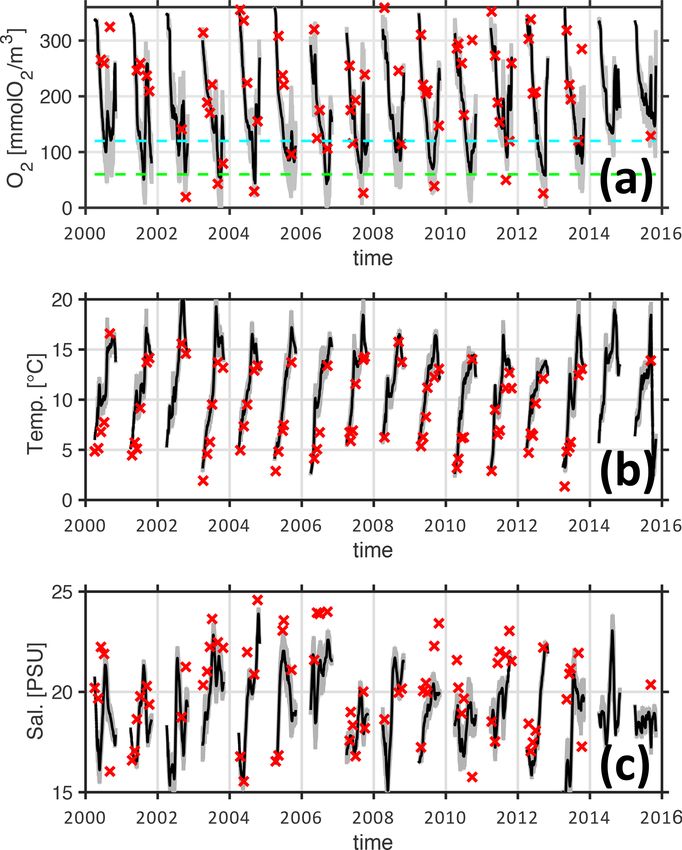
4246                                                      H. Dietze and U. Löptien: Retracing hypoxia in Eckernförde Bight

and settings identical to those applied by Dietze et al. (2014)    entering and leaving the EB. This factor will be considered
in a high-resolution model configuration of the Baltic Sea.        when analyzing the model results.
An exception is the parameter choice for the vertical back-           The water exchange across the rigid wall boundary con-
ground diffusivity: Holtermann et al. (2012) estimates from        dition is mimicked by restoring to prescribed temperature,
measurements for deep water processes in the central Baltic        salinity, and sea surface height values at the model bound-
Sea a vertical diffusivity of 10−5 m2 s−1 (calculated from         aries only. There is no restoring inside EB, and there are
the propagation speed of a purposely deployed dye-like sub-        no tides because the impact of tides is negligible in the
stance). Closer to coast Holtermann et al. (2012) report much      Baltic Sea. For sea surface height we restore it to pre-
higher values. Because mapping this information on condi-          scribed values taken from an oceanic reanalysis carried out
tions in EB is difficult, we decided to test a range of vertical   with MOMBA (Dietze et al., 2014). MOMBA differs from
background diffusivities and to assess the respective model        MOMBE in that it covers the entire Baltic Sea with a hor-
performances based on available observations. The consid-          izontal resolution of 1 nautical mile, while MOMBE intro-
ered diffusivities are 5×10⁻⁵ , 1×10⁻⁴ , and 5×10⁻⁴ m2 s−1 .       duced here covers the EB only – albeit with much higher
This range comprises relatively low diffusivities, which are       resolution (100 m). For the sake of consistency, MOMBA
characteristic for the deep central Baltic Sea, and fairly high    has been integrated for the entire hindcast period 2000–
values, which are more representative for coastal mixing (as       2018 using the atmospheric forcing described above (which
can be expected in the shallow Eckernförde Bight).                 differs from Dietze et al., 2014). For temperature, salinity,
                                                                   and oxygen we restore MOMBE at its horizontal bound-
                                                                   aries with Kiel Bight to interpolated measurements from
2.1.3   Boundary conditions
                                                                   station Boknis Eck at the entrance of EB (Lennartz et al.,
                                                                   2014, http://www.bokniseck.de/, last access: 15 July 2021,
The atmospheric boundary conditions of our model are               http://doi.pangaea.de/10.1594/PANGAEA.855693).
set by a reanalysis from the Swedish Meteorological and
Hydrological Institute (SMHI). We use the results of the           2.1.4   Sea ice
reanalysis framework as a means to interpolate (patchy)
observations in time and space. The underlying atmo-               The focus of our investigation is on ice-free seasons. We
spheric model features a horizontal resolution of 11 km.           will show in Sect. 4.1 that the memory of the system un-
For the period 2000 to 2015 we use RCA4 (Samuelsson                der consideration, as given by residence times in Eckernförde
et al., 2015, 2016). RCA4 data are available only until            Bight, is less than a month. This suggests that sea ice dynam-
2015. Hence, for the period 2016 to 2018 we switched               ics are rather irrelevant to the processes and seasons exam-
to another product: UERRA (regional reanalysis for Eu-             ined here. Even so, for the sake of completeness, we report
rope;      https://cds.climate.copernicus.eu/cdsapp#!/dataset/     that our ocean component is coupled to a dynamical sea ice
reanalysis-uerra-europe-complete?tab=overview, last ac-            module, the NOAA’s Geophysical Fluid Dynamics Labora-
cess: 15 July 2021). UERRA is more advanced but does not           tory (GFDL) sea ice simulator (SIS). The SIS uses elastic–
include “spectral nudging” to the large-scale atmospheric          viscous–plastic rheology adapted from Hunke and Dukow-
circulation. This detail may allow for unrealistic shifts in       icz (1997). We use the exact same settings described in Di-
the trajectories of low-pressure systems. Fortunately, for         etze et al. (2020) (which are identical to the settings in Dietze
the time and location under consideration here, a rough            et al., 2014, except for switching to levitating sea ice).
comparison with the observations from Kiel lighthouse (in
position 54.3344◦ N, 10.1202◦ E) showed a generally good           2.1.5   Artificial clocks
agreement between reanalysis and direct observations (not
shown).                                                            In order to facilitate the dissection of local versus remote pro-
   A key element of regional ocean circulation model con-          cesses influencing the oceanic oxygen concentrations in EB,
figurations are artificial boundary conditions introduced to       we introduce two artificial tracers or “clocks” to the ocean
limit the model domain. Typically, the choice of the extent of     circulation model (following an approach similar to Dietze
the model domain is enforced by computational capabilities         et al., 2009). Both clocks behave like dyes in that they are
rather than by scientific necessity. This can be problematic       subject to transport processes just like temperature, salinity,
because boundary conditions are known to introduce spu-            and dissolved oxygen. In addition to being transported, the
rious effects (e.g., Jensen, 1998; Blayo and Debreu, 2005;         clocks continuously count up time in every grid box. The
Herzfeld et al., 2011). Our choice is pragmatic in that we         first clock is reset to zero whenever a water parcel reaches
choose a rigid wall (such as Carton and Chao, 1999; Dietze         the ocean surface. Thus, it measures the time elapsed since a
et al., 2014). In combination with our spacial discretization      water parcel had been in contact with the atmosphere. This
(Arakawa B; Arakawa and Lamp, 1977) this necessitates a            time is also referred to as the age of the water. The second
no-slip boundary condition which removes kinetic energy.           clock is reset to zero at the eastern boundaries of the model
By this choice, we may underestimate the effect of water           domain. Thus, it measures the time elapsed since water en-

Biogeosciences, 18, 4243–4264, 2021                                                   https://doi.org/10.5194/bg-18-4243-2021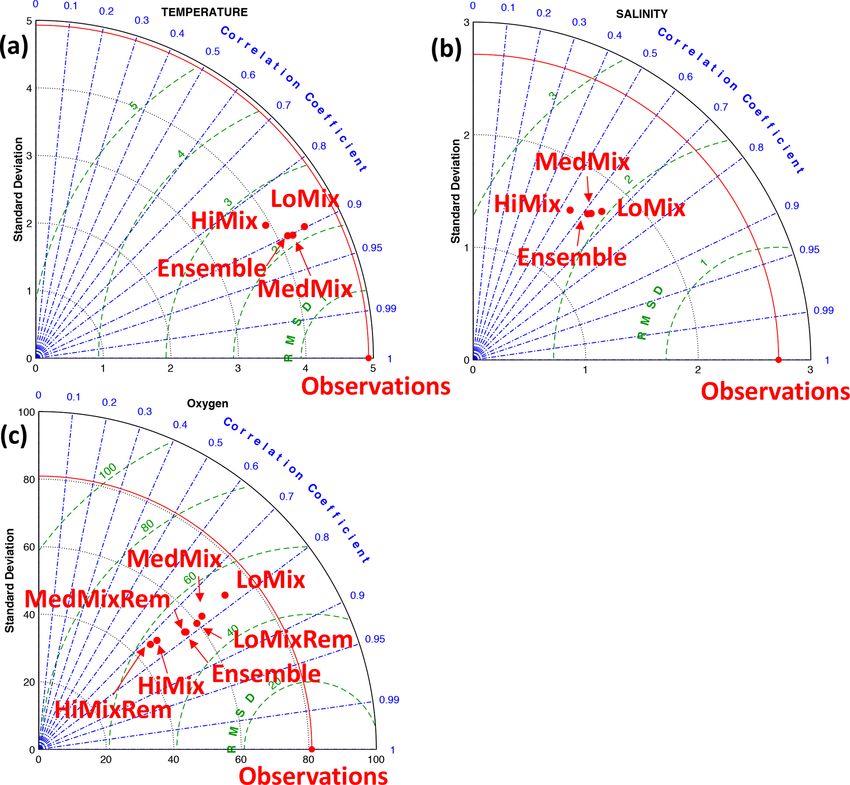
H. Dietze and U. Löptien: Retracing hypoxia in Eckernförde Bight                                                            4247

tered EB. This time is also referred to as the residence time     and define the threshold values for hypoxia as a concentration
of water in EB.                                                   of dissolved oxygen of 2 mg O2 L−1 , which corresponds to
                                                                  ≈ 60 mmol O2 m−3 . The relevance of this threshold is that it
2.1.6    Oxygen                                                   limits the survival of most fish (Hofmann et al., 2011). In ad-
                                                                  dition we consider a second threshold of 4 mg O2 L−1 corre-
Our dissolved oxygen module is dubbed EckO2 module                sponding to ≈ 120 mmol O2 m−3 . This value is used as an in-
(from Eckernförde O2 ). The module is very similar to the         dicator for the eutrophication of stratified water bodies (such
OXYCON approach that Bendtsen and Hansen (2013) used              as EB) by the Baltic Marine Environment Protection Com-
and also Lehmann et al. (2014). A schematic representation        mission (Helsinki Commission – HELCOM, 16th Meeting of
of EckO2 is given in Fig. 3. Following Bendtsen and Hansen        the Intersessional Network on Eutrophication Helsinki, Fin-
(2013), the local development over time of dissolved oxygen,      land, 29–30 January 2020), and as such it is of relevance to
∂O2
 ∂t , is defined by                                               the stakeholder LLUR.
∂O2
      = A(O2 ) + D(O2 ) + S(O2 ),                           (1)
  ∂t
where A und D denote the divergence of the 3-D advective          3   Ensemble generation
and diffusive fluxes as calculated by the GCM. S denotes bio-
geochemical oxygen sources and sinks given by the model           Among the challenges in simulating oxygen dynamics is
parameters opro at the sunlit sea surface, by orewa at depth      that both biotic parameters (determining oxygen respiration;
below the compensation depth zco, and by orese in the low-        Sect. 2.1.6) and the antagonistic abiotic parameters (that con-
ermost wet model grid box. These parameters determine how         trol ventilation with surface water high in oxygen such as, for
much oxygen is generated by primary production (opro) and         example, vertical diffusivity; Sect. 2.1.2) are uncertain. Our
how much is consumed at depth (orewa) and in the sediment         approach is to run an ensemble of simulations encompass-
(orese). The respective parameter choices are based on litera-    ing a plausible range of settings. These settings are listed in
ture values listed in Table 1. Following Babenerd (1991) and      Table 2. We compare low, medium, and high levels of dif-
based on Ærtebjerg et al. (1981) we assume that the subsur-       fusivity (tagged LoMix, MedMix, and HighMix, respectively)
face oxygen consumption rates are rather uniform throughout       and, further, simulations which totally neglect local sources
KB, EB, and up into the Danish straits. This assumption is        and sinks of oxygen (tagged Rem for “remote biotic effects
necessitated by our lack of direct measurements of consump-       only”) versus those featuring a best guess of local sources
tion rates in EB. EckO2 prescribes climatological monthly         and sinks that are on the higher end of published estimates
mean consumption rates.                                           (cf. Table 1 with Table 2). This section identifies the most re-
   Note that our choice of oxygen consumption rates (Ta-          alistic simulations which will be considered in the following.
ble 2) corresponds to a best guess at the higher end of pub-      The ultimate goal is to chose parameter settings which cover
lished estimates (Table 1). To this end the simulations includ-   the contemporary uncertainty range.
ing these local sources and sinks of oxygen provide an upper         Figure 4 shows Taylor diagrams which compare simulated
bound on the effects of local biotic processes on local oxygen    and observed temperature, salinity, and oxygen. The simula-
dynamics in EB. A lower bound is explored by setting local        tions with high diffusivity (HiMix and HiMixRem) feature the
consumption and production to zero.                               lowest performance in reproducing the observed variability
                                                                  in temperature, salinity, and oxygen. This is consistent with
2.2     Observations                                              an assessment of simulated velocities by Marlow (2020). We
                                                                  thus discard these simulations from the analysis. The more
We use data from the regular monitoring program of the Lan-       realistic simulations LoMix and HiMix are very similar irre-
desamt für Landwirtschaft, Umwelt und ländliche Räume             spective of whether we account for local sources and sinks
(LLUR). Respective approximate monthly observations of            of oxygen or not. We conclude (from Fig. 4) that the lower
salinity, temperature, and oxygen covered the entire hindcast     values for the diffusivity are more realistic and that local
period at the monitoring station Buoy 2a (location marked         sources and sinks of oxygen are apparently of minor impor-
in Fig. 2). Typical surface concentrations of dissolved oxy-      tance within EB.
gen are around a few hundred millimoles O2 per cubic me-             Figure 5 shows simulated and observed oxygen concentra-
ter (mmol O2 m−3 ), predominantly set by physical solubility      tions at the bottom of the monitoring station Buoy 2a for the
as a function of temperature and salinity (and rather con-        years 2000–2015. The respective months of April to October
stant atmospheric concentrations). At depth, however, oxy-        are shown. November to March are omitted because these
gen sinks can accumulate oxygen deficits until critical thresh-   months feature high concentrations of dissolved concentra-
olds for the survival of animal or even plants are under-         tions beyond our scope of interest. The overall impression is
cut. Common denominations for critical thresholds are hy-         that the model retraces the dynamics of temperature, salin-
poxic, suboxic, and anoxic conditions. Their respective val-      ity, and oxygen reasonably well. Figure 6 provides a more
ues are, however, fuzzy. Here, we follow Gray et al. (2002)       quantitative estimate of the fidelity in reproducing hypoxic

https://doi.org/10.5194/bg-18-4243-2021                                                  Biogeosciences, 18, 4243–4264, 2021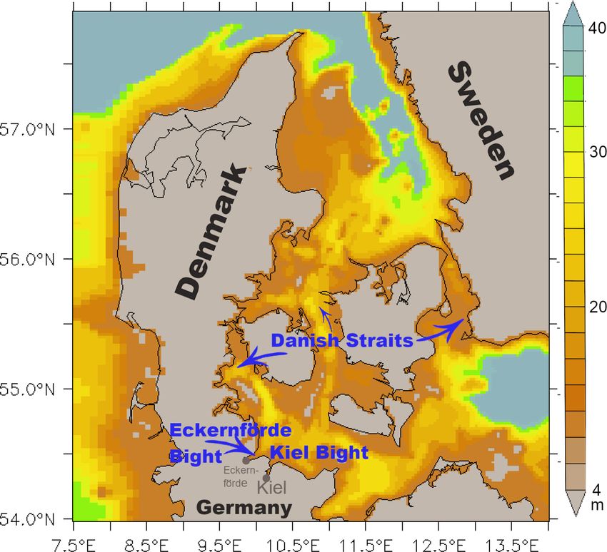
4248                                                        H. Dietze and U. Löptien: Retracing hypoxia in Eckernförde Bight

Figure 3. Schematic of dissolved oxygen module EckO2 . EckO2 calculates sinks and sources of oxygen throughout the water column
for every grid box. These terms are then passed to the 3-D general ocean circulation that handles the effect of advection and diffusion.
The velocity of the air–sea gas exchange is determined by the piston velocity kgt. Above the compensation depth zco, primary production
produces oxygen at a rate prescribed by the model parameter opro. Below the compensation depth zco, respiration of organic matter consumes
dissolved oxygen at a rate prescribed by orewa. At the bottom, prescribed oxygen fluxes orese mimic the oxygen consumption of the sediment
that is fueled by the transfer across the water–sediment boundary. Table 2 summarizes respective parameter settings.

events (as defined by the 120 mmol O2 m−3 introduced in                entrance of EB to forecast hypoxia within EB at the monitor-
Sect. 1) at the monitoring station Buoy 2a. It shows sensitiv-         ing station Buoy 2a.
ity and specificity achieved with the simulations LoMix and
MedMix that account for local sources and sinks of oxygen:             4.1   Residence and ventilation times
LoMix typically simulates ≈ 70 % true positives and ≈ 10 %
false positives. MedMix, in comparison, simulates only sev-
eral percent false positives but fails to identify every third         The estimates of residence and ventilation times are calcu-
event (i.e., ≈ 70 % true positives).                                   lated with “artificial clocks”, as described in Sect. 2.1.5. Both
                                                                       model versions LoMix and MedMix show similar results: the
                                                                       water with the longest residence time is found at the end of
                                                                       EB in the interior close to the city of Eckernförde (Fig. 7).
4   Results                                                            Typical values are of the order of 1 month for both exemplary
                                                                       months, August and October. Overall, MedMix shows lower
We start with exploring the simulated residence and venti-             values than LoMix indicating that vertical diffusive processes
lation timescales (Sect. 4.1) for the simulations LoMix and            promote the horizontal exchange of water between EB and
MedMix. This provides a base for understanding the dynam-              KB. This makes sense because the longest residence times
ics behind our hindcast presented in Sect. 4.2. A complemen-           can be found at the surface (Fig. 8), suggesting that, on av-
tary case study of the intense hypoxic event 2017 is presented         erage, water enters the bight at depth and leaves the bight at
in Sect. 4.3. Section 4.4 describes the application of artificial      the surface. A stronger vertical diffusivity is then associated
intelligence for feature selection and extraction of the predic-       with an accelerated rate of surface water renewal by deep
tive capability of monitoring data at station Boknis Eck at the        water with shorter residence times.

Biogeosciences, 18, 4243–4264, 2021                                                        https://doi.org/10.5194/bg-18-4243-2021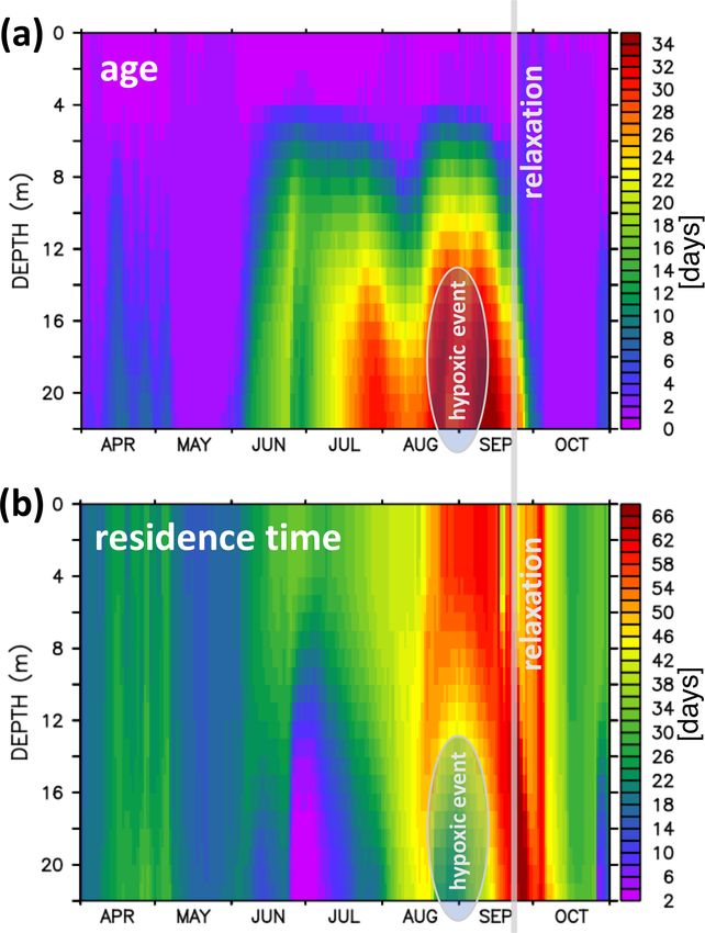
H. Dietze and U. Löptien: Retracing hypoxia in Eckernförde Bight                                                                            4249

Table 1. Estimates of oxygen consumption and production converted to respective model parameters of the EckO2 module. Conversions may
include division by the average water depth and area of Eckernförde Bight (see Sect. 2.1.1), a O2 : C ratio of 1.1, and a C : P ratio of 106.

   Reference                    Description                                                    opro               orewa                 orese
                                                                                  (mmol O2 m−2 d−1 )   (mmol O2 m−3 d−1 )   (mmol O2 m−2 d−1 )
   Babenerd (1991)              In situ measurements during summer strat-                                            3.75
                                ification 1985 and 1986 at the monitoring
                                station Boknis Eck
   Bendtsen and Hansen (2013)   Prescribed parameters in a model of the                         2.75                 0.36                  3.1
                                Baltic Sea–North Sea transition which
                                yielded a good fit to observed oxygen con-
                                centrations
   Rahm (1987)                  Budget calculations for the Baltic Proper                                            0.26
   Noffke et al. (2016)         In situ measurements with a lander in the                                                             5.8–20.8
                                eastern Gotland Basin
   Pers and Rahm (2000)         Budget calculations for the Baltic Proper                                         1.1–2.4
   Smetacek (1980, 1985)        In situ measurements in the western Kiel                                                                   1.6
                                Bight with detritus traps in June (assuming
                                negligible fraction of permanent burial)
   Smetacek (1980, 1985)        In situ measurements in the western Kiel                                                                   6.3
                                Bight with detritus traps in August (assum-
                                ing negligible fraction of permanent burial)
   Haustein (2002)              Average (dry days) oxygen consumption                                                0.04
                                equivalent of Kiel Bülk sewage effluent,
                                distributed evenly over Eckernförde Bight
   Haustein (2002)              Episodic, extreme discharge event during                                             0.36
                                18 and 19 July 2002 of the Kiel Bülk
                                sewage plant, converted into oxygen con-
                                sumption equivalent distributed evenly over
                                Eckernförde Bight
   Nausch et al. (2011)         Average Kiel Bülk sewage phosphorous ef-                                             0.03
                                fluent, converted into oxygen consumption
                                assuming that it fuels organic matter pro-
                                duction that is remineralized in Eckernförde
                                Bight
   Nausch et al. (2011)         Phosphorous loads of rivulet Schwentine                                              0.18
                                that drains into Kiel Bight, converted into
                                oxygen consumption assuming that it fu-
                                els organic matter production that is entirely
                                remineralized at depth in Eckernförde Bight

   The distribution of ventilation times or age is similar to                    oxygenated surface waters. Biogeochemical processes in the
that of residence times in that the highest values are generally                 interior of EB are apparently of minor importance for the
found within the bight towards Eckernförde (Fig. 9). The hor-                    oxygen dynamics within EB.
izontal gradient is more pronounced in the simulation with
lower mixing, while higher prescribed vertical background                        4.2   The typical seasonal cycle inside EB
mixing equalizes the effective ventilation processes horizon-
tally. In terms of vertical distribution, age has, in contrast to                Figure 5 shows a comparison between the observed and sim-
the residence time, high values at depth and low at the sur-                     ulated temporal evolution of dissolved oxygen concentra-
face, where it is reset to zero (Fig. 10).                                       tions at the bottom of the monitoring station Buoy 2. Most
   In summary, we find that residence times and age are of                       prominent is a pronounced seasonal cycle. The generic expla-
similar magnitude. This suggests that the first order control                    nation for such seasonal cycles in such latitudes is that tem-
of processes that determine oxygen concentrations in EB is                       peratures and biomass production in the surface waters ramp
an antagonistic interplay of inflowing water (generally low                      up in spring, being driven by enhanced levels of photosyn-
in oxygen) and the local aeration by vertical exchange with                      thetically available radiation (note, however, that there is an

https://doi.org/10.5194/bg-18-4243-2021                                                                 Biogeosciences, 18, 4243–4264, 2021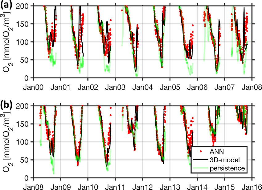
4250                                                           H. Dietze and U. Löptien: Retracing hypoxia in Eckernförde Bight

Table 2. List of model parameter settings for the EckO2 module and diffusive background mixing in MOMBE: κv refers to vertical back-
ground mixing (diffusivity), and opro, orewa, and orese refer to monthly (one value per month starting with the January value) oxygen
production, water column oxygen respiration, and oxygen consumption by the sediment, respectively (cf. Fig. 3). Values for orewa and orese
are derived from the published estimates listed in Table 1; opro is calculated as residual assuming instant equilibration of sedimentary fluxes.

    Tag              Description                                   κv     opro               orewa              orese
                                                             (m2 s−1 )    (mmol O2 m−2 d−1 ) (mmol O2 m−3 d−1 ) (mmol O2 m−2 d−1 )
    LoMix            Low vertical background mixing of       5 × 10⁻⁵     48 47 47 46 46 45      3.8 3.8 3.8 3.8 3.8    4 3.5 3 2.5 2.1 1.6
                     momentum and tracers. Local oxy-                     48 50 50 49 48 48      3.8 3.8 3.8            3.95 6.3 5.8 5.4 4.9
                     gen consumption and production                                                                     4.4
                     rates at the upper limit of published
                     estimates.
    LoMixRem         Low vertical background mixing of       5 × 10⁻⁵     0000000000             0000000000             0000000000
                     momentum and tracers. No local                       00                     0                      00
                     oxygen consumption and produc-
                     tion.
    MedMix           Medium vertical background mix-         1 × 10⁻⁴     48 47 47 46 46 45      3.8 3.8 3.8 3.8 3.8    4 3.5 3 2.5 2.1 1.6
                     ing of momentum and tracers. Lo-                     48 50 50 49 48 48      3.8 3.8 3.8            3.95 6.3 5.8 5.4 4.9
                     cal oxygen consumption and pro-                                                                    4.4
                     duction rates at the upper limit of
                     published estimates.
    MedMixRem        Medium vertical background mix-         1 × 10⁻⁴     0000000000             0000000000             0000000000
                     ing of momentum and tracers. No                      00                     0                      00
                     local oxygen consumption and pro-
                     duction.
    HiMix            High vertical background mixing         5 × 10⁻⁴     48 47 47 46 46 45      3.8 3.8 3.8 3.8 3.8    4 3.5 3 2.5 2.1 1.6
                     of momentum and tracers. Local                       48 50 50 49 48 48      3.8 3.8 3.8            3.95 6.3 5.8 5.4 4.9
                     oxygen consumption and produc-                                                                     4.4
                     tion rates at the upper limit of pub-
                     lished estimates.
    HiMixRem         High vertical background mixing of      5 × 10⁻⁴     0000000000             0000000000             0000000000
                     momentum and tracers. No local                       00                     0                      00
                     oxygen consumption and produc-
                     tion.

ongoing discussion on this issue: Behrenfeld, 2010; Arteaga                  Based on the hindcast simulation from 2000 to 2015 hy-
et al., 2020; Smetacek, 1985). The biomass eventually sinks               poxic events at station Buoy 2a are most common in Au-
to depth where it degrades and issues oxygen consumption.                 gust and October with a local minimum of occurrences in
Later in the season, the water column stratifies, and the sur-            September (Fig. 11). This is inconsistent with the generic ex-
face layer heats up, effectively creating a barrier to the ex-            planation outlined above, where a period of ever decreasing
change of bottom water (deprived of oxygen) and the oxy-                  levels of dissolved oxygen ends in autumn when increasing
genated surface waters. As autumn approaches, the surface                 winds and a pronounced air–sea heat transfer promotes net
ocean cools again and weakens the stratified barrier to ver-              ventilation. So why do hypoxic conditions deep in EB at sta-
tical mixing. This facilitates the wind-driven mixing events              tion Buoy 2a become more frequent after the September set-
that come along with more unstable autumn weather. In win-                back despite increasing winds and decreasing thermal strat-
ter, convective mixing homogenizes the entire (rather shal-               ification? The histograms of bottom oxygen concentrations
low) water column vertically (e.g., Fennel and Testa, 2019;               observed at station Boknis Eck, situated at the entrance to
Petenati, 2017). Apparently the model captures this dynamic               EB (and used to prescribe the conditions of water flowing
well; i.e., the ensemble mean of LoMix and MedMix features                into EB in the model), suggest that particularly low oxygen
a high visual correspondence between the respective curves                concentrations are more frequent in October than in August
in Fig. 5 (see Fig. 4 for more quantitative estimate).                    (Fig. 12). Hence, water entering EB from KB in October
                                                                          is more likely to “import” hypoxia. Note that these consid-

Biogeosciences, 18, 4243–4264, 2021                                                            https://doi.org/10.5194/bg-18-4243-2021
H. Dietze and U. Löptien: Retracing hypoxia in Eckernförde Bight 4251
Figure 4. Model assessment (Taylor plots) at station Buoy 2a in the interior of EB (Fig. 2). Observational data and model output refer to
the 2000 to 2015 period. The simulation tags are defined in Table 2: LoMix, MedMix, and HiMix denote the levels of diffusive background
mixing. Rem indicates remote effects of biogeochemical sources and sinks of oxygen only (i.e., no local oxygen consumption in EB.
erations are in line with simulations LoMixRem/LoMix and The notion of “imported” hypoxic conditions is backed by
MedMixRem/MedMix, each pair showing in Fig. 4 very little the Hovmöller diagrams of simulated age and residence
effect of local oxygen consumption within EB, even though times at the monitoring station Buoy 2a in Fig. 14: dur-
(1) the respective biotic local oxygen consumptions are cho- ing the buildup of the hypoxic event in EB, the residence
sen to represent the upper limit of published estimates and time features a local minimum deep inside EB. This suggests
(2) the water exchange with KB is hampered by a rigid wall the prevalence of water masses “recently imported” from
boundary condition. KB (Fig. 14b). Simultaneously, the age features a maximum
We conclude that the typical oxygen deficit in late sum- (Fig. 14a), indicating that the recently imported hypoxic wa-
mer is imported along with water from the KB, rather than ters are well shielded from ventilation by oxygenated sur-
being produced locally in EB. The following Sect. 4.3 will face waters. Further evidence is provided in Fig. 15, show-
elucidate the underlying succession of events by means of a ing that the oxygen decline in EB is contemporaneous with
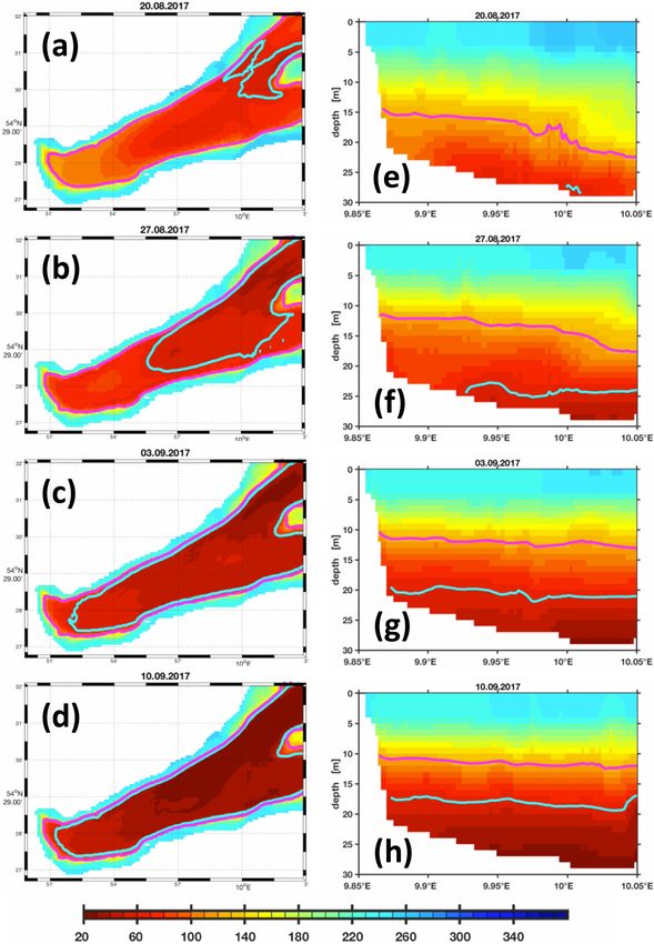
detailed case study. winds blowing out of the bight. These winds drive an over-
turning circulation, shown in Fig. 16, with surface waters be-
4.3 Hypoxic event 2017 ing pushed out of the bight and bottom waters, for continuity
reasons, being sucked into the bight at depth. Consequently,
In fall 2017 a particularly pronounced hypoxic event oc- we find in Fig. 15 that the oxygen decline at the entrance
curred and led to a mass fish-kill incidence. In the following, of the bight (at station Boknis Eck) occurs earlier than the
we analyze this event in the MOMBE LoMix simulation. oxygen decline inside the bight (at station Buoy 2a) – just
Figure 13 shows a sequence of snapshots of simulated hy- as expected in a system where water enters the bight at the
poxia in EB, starting 20 August and ending at peak con- bottom.
ditions on 10 September. Over the course of these several During the relaxation phase that terminates the 2017 hy-
weeks, EB loses oxygen, and hypoxic waters apparently en- poxic event, the processes are reversed: Fig. 17 shows that the
ter the bight at the bottom from the east and move upwards. winds are blowing consistently into the bight for more than
https://doi.org/10.5194/bg-18-4243-2021 Biogeosciences, 18, 4243–4264, 2021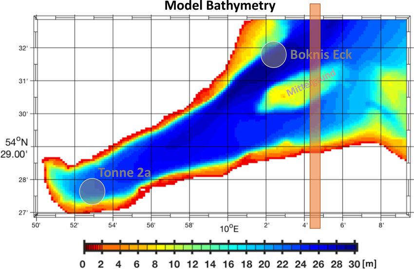
4252                                                         H. Dietze and U. Löptien: Retracing hypoxia in Eckernförde Bight

                                                                      Figure 6. Fidelity of hindcasted hypoxic events (oxygen threshold
                                                                      of 120 mmol O2 m−3 ) at station Buoy 2a.

                                                                      for netting and landing of doomed fish. The following section
                                                                      applies artificial intelligence (AI) to pursue these questions.

                                                                      4.4   AI-based feature selection and time series
Figure 5. Simulated and observed oxygen concentrations at the bot-          prediction
tom (20 m depth) of the monitoring station Buoy 2a. Panels (a–c)
refer to oxygen concentrations, temperature, and salinity, respec-    The following section explores the statistical relations be-
tively. Red crosses denote observations. The black line denotes the   tween the simulated time series at station Buoy 2a deep in the
ensemble mean of the simulations MedMix and LoMix. The gray           bight and Boknis Eck at the entrance of the bight. The major
line envelopes the ensembles’ extremes at any given time. The hor-    aims are (1) to gain further mechanistic insight and (2) to de-
izontal dashed cyan and green lines in panel (a) show 120 and
                                                                      velop a surrogate model for the stakeholder that may be im-
60 mmol O2 m−3 hypoxia thresholds, respectively.
                                                                      plemented on off-the-shelf desktop computers, smart phones,
                                                                      or even on very low cost (< 10 EUR) embedded devices
                                                                      rather than necessitating access to a super-computing facil-
                                                                      ity (as is the case with the full-fledged coupled model). This
a week. Consequently, water is pushed into the bight at the           section is motivated by recent and encouraging success in
surface, having nowhere to go. Some of the well-oxygenated            emulating general circulation models (e.g., Castruccio et al.,
surface water is subducted to depth and subsequently leaves           2014), ecosystem models (e.g., Fer et al., 2018), the tremen-
EB at depth. Just as expected, the increase in oxygen at the          dous success in machine learning and data-driven methods
monitoring station Buoy 2a inside the bight occurs earlier            in fluid dynamics (as summarized, for example, by Brunton
than the corresponding oxygen increase at the entrance sta-           et al., 2020a), and the sneaking suspicion that “. . . the most
tion Boknis Eck. The oxygen levels at Boknis Eck now lag              pressing scientific and engineering problems of the modern
behind Buoy 2a by approximately 1 week.                               era are not amenable to empirical models or deviations of
   In summary, we identified a governing mechanism by                 first principles. . . ” (Brunton et al., 2020b).
which EB is – depending on wind direction – either (1) im-               In the following, we describe the application of shallow
pacted by imported low-oxygenated waters from KB or (2)               and deep feed-forward artificial neural networks (ANNs) to
being flushed by oxygenated surface water that is subducted           forecast bottom oxygen concentrations deep inside EB at the
to depth in the interior of EB and is exported at depth to KB         Buoy 2a monitoring station 2 weeks in advance from the at-
– whereby EB is effectively ventilating KB.                           mospheric conditions and the regularly sampled monitoring
   Open questions, however, remain. Of particular interest            station Boknis Eck at the entrance of the bight. The forecast
is the questions of why some years are hit especially hard            range is chosen as a compromise between the time needed for
by hypoxia and whether such events are predictable days or            mitigation measures (e.g., by netting and landing of doomed
weeks in advance. Such predictions may, for example, allow            fish) and forecast accuracy which typically degrades with

Biogeosciences, 18, 4243–4264, 2021                                                      https://doi.org/10.5194/bg-18-4243-2021
H. Dietze and U. Löptien: Retracing hypoxia in Eckernförde Bight 4253
Figure 7. Simulated climatological estimate of the residence time of water parcels in EB. The units are days elapsed since the water flushed
into the bight. The estimate refers to the longest residence time found in local water columns. Panels (a) and (b) refer to August calculated
by the simulations LoMix and MedMix, respectively. Panels (c) and (d) refer to October calculated by the simulations LoMix and MedMix,
respectively. Note that the model domain extends beyond the eastern boundary shown here (see also Fig. 2).
Figure 8. Simulated climatological estimate of the residence times of water parcels in EB. The units are days elapsed since the water
flushed into the bight. Sections along EB are shown. Panels (a) and (b) refer to August calculated by the simulations LoMix and MedMix,
respectively. Panels (c) and (d) refer to October calculated by the simulations LoMix and MedMix, respectively. Note that the model domain
extends beyond the eastern boundary shown here (see also Fig. 2).
forecasting range. During the course of this exercise we will methods (Makridakis et al., 2018), is beyond the scope of this
use different combinations of predictors (or input data) and article.
test their impact on the forecast skill – a process also re-
ferred to as capacity estimation and feature selection (e.g., 4.4.1 Capacity estimation and feature selection
Sbalzarini et al., 2002). Note, however, that a comprehensive
analysis of time series forecasting, which must include tradi-
For training the ANNs, we draw our training (80 %) and val-
tional statistical approaches in addition to machine learning
idation data (20 %) randomly from the 2000 to 2016 model
https://doi.org/10.5194/bg-18-4243-2021 Biogeosciences, 18, 4243–4264, 20214254 H. Dietze and U. Löptien: Retracing hypoxia in Eckernförde Bight Figure 9. Simulated climatological estimate of local ventilation. The color shading denotes the time elapsed (age) since bottom water has been in contact with the atmosphere in units of days. Panels (a) and (b) refer to August calculated by the simulations LoMix and MedMix, respectively. Panels (c) and (d) refer to October calculated by the simulations LoMix and MedMix, respectively. Note that the model domain extends beyond the eastern boundary shown here (see also Fig. 2). Figure 10. Simulated climatological estimate of local ventilation. The color shading denotes the time elapsed (age) since water parcels have been in contact with the atmosphere in units of days. Sections along EB are shown. Panels (a) and (b) refer to August calculated by the simulations LoMix and MedMix, respectively. Panels (c) and (d) refer to October calculated by the simulations LoMix and MedMix, respectively. Note that the model domain extends beyond the eastern boundary shown here (see also Fig. 2). hindcast. We hand-design features (input data) and test their provide a lower bound on the potential of ANNs for the task respective capacity to forecast bottom oxygen concentrations at hand. at station Buoy 2a (target data). Hand-designed features are The ANN is trained using the Levenberg–Marquardt al- “. . . two edged swords” (e.g., Reichstein et al., 2019): they gorithm (Marquardt, 1963) applied to neural network train- can be seen as an advantage because they give us control of ing following Hagan and Menhaj (1994) and Hagan et al. the explanatory drivers which may be used to promote sys- (1996). Each training is repeated 30 times, each of which tem understanding. On the other hand, hand-designed fea- may yield (slightly) differing results because, depending on tures are typically suboptimal. To this end our results here the (random) initialization of weights, the algorithm may ter- Biogeosciences, 18, 4243–4264, 2021 https://doi.org/10.5194/bg-18-4243-2021
H. Dietze and U. Löptien: Retracing hypoxia in Eckernförde Bight                                                                4255

                                                                      forecast totaling 106 input features (given by the three 1 m
                                                                      resolution vertical profiles of temperature, salinity, and oxy-
                                                                      gen down to 26 m depth and the 14 daily forecasts of zonal
                                                                      and meridional winds each). This setup is based on an opti-
                                                                      mistic estimate of the number of features available to stake-
                                                                      holders. Specifically, we assume to have access to a correct
                                                                      biweekly wind forecast along with one full vertical profile
                                                                      each of temperature, salinity, and oxygen at the monitoring
                                                                      station Boknis Eck located at the entrance of EB (i.e., the 106
Figure 11. Simulated climatological (2000–2015) occurrence of         features introduced above).
hypoxia at the monitoring station Buoy 2a. Occurrence refers to the
                                                                         Figure 18 suggests that the Pareto Frontier is at 45 %, cor-
sum of suboxic (i.e., < 120 mmol O2 m−3 ) model grid boxes, iden-
                                                                      responding to a 55 % reduction in error relative to the persis-
tified in climatological daily model output. From November to June
suboxic conditions were absent.                                       tence model. A total of 80 % of this yields a Pareto Optimal
                                                                      of 56 %. This corresponds to one or two nodes. Additional
                                                                      tests with deeper ANNs featuring up to 10 hidden layers with
                                                                      two nodes were unsuccessful in that respective errors were
                                                                      always higher than 50 %. We conclude that a simple two node
                                                                      shallow ANN already features a reasonable performance, and
                                                                      two input features, of the 106 tested, may suffice to capture
                                                                      the main effects.
                                                                         Table 3 summarizes our effort to identify the most pre-
                                                                      dictive features by backward elimination (e.g., Dietterich,
                                                                      2002). Using combinations of only 15 features comprised of
                                                                      biweekly zonal wind speed and the bottom values of either
                                                                      temperature, salinity, or oxygen yielded a moderate degra-
                                                                      dation in performance of only 10 % (Table 3 entries 2 to 4).
                                                                      Pushing further we identified a combination of two features
                                                                      only that are, on the one hand, within this 10 % degradation
Figure 12. Histogram of observed climatological bottom oxygen         and, on the other hand, especially easy to measure for stake-
concentrations at Boknis Eck (capped at 100 mmol O2 m−3 ).            holders: surface and bottom temperatures at station Boknis
                                                                      Eck. Contrary to intuition, adding wind forecasts does not
                                                                      improve the ANNs fidelity (compare entries 5 and 6 in Ta-
minate in potentially differing local optima of the cost func-        ble 3). Even so, the ANN fits the training and validation data
tion. As cost function we choose mean-squared errors (calcu-          remarkably well (Fig. 19). We conclude that the ANN’s bi-
lated from MOMBE output and the ANN prediction designed               weekly forecast exploits links other than those being direct
to mimic the MOMBE output). Figure 18 shows respective                consequences of the wind-driven inflow versus ventilation
cost as errors relative to a naive biweekly persistency fore-         mechanism identified in Sect. 4.3. Section 4.4.2 puts this ex-
cast based on bottom oxygen concentrations at the monitor-            ploitation to the test using independent test (model) data.
ing station Boknis Eck: apparently the ANN’s performance
converges at 45 % relative to the persistency forecast. Defin-        4.4.2   ANN generalization
ing this as the Pareto frontier suggests a Pareto optimal of
56 %, which corresponds to one or two nodes. The idea of              This section discusses the fidelity of the two-node ANN us-
opting for a rather parsimonious two-node model that scores           ing simulated bottom and surface temperatures identified in
80 % of the Pareto Frontier rather than 100 % is to reduce the        Sect. 4.4.2 as being parsimonious but – nevertheless – yield-
risk of overfitting which may hinder generalization. Further,         ing reasonable results compared to more complex architec-
parsimonious models are easier to interpret than their com-           tures, such as deeper nets using more nodes and input data.
plex counterpart such that their robustness is easier to assess.      Here, we use independent test data covering the years 2016 to
This is especially important because we have no straightfor-          2018 of our hindcast simulation. These data have been used
ward way to extract human semantics from the “rules” the              neither in training nor during validation so far. To rate the
neural network learned during the optimization process that           forecast it is compared to the “persistence model”, which as-
related our input features to the target bottom oxygen con-           sumes that the oxygen concentrations at station Boknis Eck
centrations at station Buoy 2a.                                       appear 2 weeks later at station Buoy 2a (green line in Fig. 20).
   We start with a shallow (one input, one hidden, and one            The first striking impression of the close-ups in Fig. 20 is
output layer) ANN utilizing the full vertical profiles of tem-        that all years feature a similar seasonal decline in bottom
perature, salinity, and oxygen along with a biweekly wind             oxygen in autumn and this decline generally closely resem-

https://doi.org/10.5194/bg-18-4243-2021                                                      Biogeosciences, 18, 4243–4264, 2021
4256 H. Dietze and U. Löptien: Retracing hypoxia in Eckernförde Bight Figure 13. Simulation (LoMix) of the 2017 hypoxic event. The colors refer to oxygen concentrations (in mmol O2 m−3 ). The contours in cyan and magenta show the 60 and 120 mmol O2 m−3 isolines. The left column (a–d) shows oxygen concentrations on the sea floor. The right column (e–h) shows a section through the bight with the city of Eckernförde to the left and the entrance to the bight to the right. (Corresponding animations featuring daily resolution named LoMix_O2_Bottom_2015.m4v and LoMix_O2_zonal_2017.m4v are archived at https://doi.org/10.5281/zenodo.4271940.) Note that the model domain extends beyond the eastern boundary shown here (see also Fig. 2). bles the oxygen decline in Boknis Eck 2 weeks in advance. Ventilation, however, takes place in the interior of the bight, Large interannual differences, however, occur at the onset and its signal reaches station Boknis Eck at the entrance af- of the trend reversal. This “return point” in time is not cap- terwards such that we indeed expect no predictive power of tured well by the persistency model. These results are con- the persistency model under these circumstances. To this end, sistent with our results in Sect. 4.3 showing that the decline our ANN clearly outperforms the persistency model in that it is driven by the import of low-oxygenated waters from KB. predicts an earlier and more realistic recovery of oxygen val- Biogeosciences, 18, 4243–4264, 2021 https://doi.org/10.5194/bg-18-4243-2021
H. Dietze and U. Löptien: Retracing hypoxia in Eckernförde Bight                                                                       4257

Table 3. Capacity estimation of input features. This table relates the fidelity of biweekly walk-forward ANN forecasts of bottom oxygen
concentrations at the monitoring station Buoy 2a with data from station Boknis Eck fed to the ANN. The average of wind speed squared
refers to respective biweekly forecasts of zonal winds. The error is the RMS deviation between the (computationally cheap) ANN projection
and simulated (computationally expensive; full-fledged coupled biogeochemical ocean circulation model) bottom oxygen concentrations at
Buoy 2a relative to the respective RMS of the persistence model (which naively assumes that Boknis Eck bottom oxygen concentrations will
persist for 14 d at Buoy 2a.

                         Input features                                                                Error (%)
                         Average of zonal and meridional wind speed squared, full vertical profiles            54
                         (26 depth levels) of O2 , temperature, and salinity
                         Average of zonal wind speed squared, bottom O2                                        64
                         Average of zonal wind speed squared, bottom salinity                                  65
                         Average of zonal wind speed squared, bottom temperature                               62
                         Average of zonal wind speed squared, surface and bottom temperatures                  58
                         Surface and bottom temperatures                                                       58

                                                                       Figure 15. Simulated temporal evolution of (a) wind direction,
                                                                       (b) wind speed, and (c) bottom oxygen concentrations during the
Figure 14. Hovmöller diagrams of simulated water age and res-
                                                                       buildup of the 2017 hypoxic event. The black and red lines in
idence time at the monitoring station Buoy 2a (a and b, respec-
                                                                       panel (c) refer to station Boknis Eck at the entrance and station Buoy
tively). The oval marking in August–September highlights the 2017
                                                                       2a deep inside EB, respectively.
hypoxic event. The vertical gray line marks the start of the relax-
ation phase ending the hypoxic event.

                                                                       and stratification (“derived” from the temperature difference
                                                                       between surface and depth) at the entrance of the bight with
ues during the end of summer/beginning of autumn despite               oxygen concentration in the interior of the bight – without
the ANN also exclusively relying on data at the entrance at            utilizing information on winds. This clearly emphasizes the
station Boknis Eck.                                                    role of stratification in putting an end to hypoxic events: EB
   The ANN essentially and successfully links information              is in the latitudes of prevailing westerlies, with “prevailing”
regarding season (“derived” from sea surface temperature)              entailing that the local winds shift back and forth as the

https://doi.org/10.5194/bg-18-4243-2021                                                         Biogeosciences, 18, 4243–4264, 2021
4258 H. Dietze and U. Löptien: Retracing hypoxia in Eckernförde Bight
Figure 17. Simulated temporal evolution of (a) wind direction, (b)
wind speed, and (c) bottom oxygen concentrations during the relax-
ation phase that terminates the 2017 hypoxic event. The black and
red lines in panel (c) refer to station Boknis Eck at the entrance and
station Buoy 2a deep inside EB, respectively.
Figure 16. Simulated, daily mean zonal currents during the buildup
of the 2017 hypoxic event shown in Figs. 13–15. Green to blue
colors characterize flows to the east (towards the KB). Yellow to
red colors indicate flows to the west (into EB). The unit is kilo-
meters per day (km d−1 ). The depicted section has an extension of
≈ 13 km. Note that the model domain extends beyond the eastern
Figure 18. ANN error relative to naive persistency forecast versus
boundary shown here (see also Fig. 2).
the number of neurons in the hidden layer. The black line features
the best ANN parameter setting found within an ensemble of 30
optimizations for each of the number of neurons tested. The gray
bars denote the ensemble’s standard deviations.
weather systems travel east. Any of these wind shifts from
westerly to easterly may end an hypoxic event in EB – if the
stratification is weak enough (and winds are strong enough) which ends hypoxic events. Given that the EM is positioned
such that oxygenated surface water can be pushed to depth. in the prevailing westerlies, the winds regularly change to
In a nutshell, if the stratification has sufficiently weakened, easterlies, but this only drives substantial oxygenation (re-
you know that the next wind shift will subduct oxygenated placement) of bottom waters if the stratification is weak
water, thereby ending the hypoxic event. enough to be penetrated. Hence, there is a high explanatory
In summary, the ANN features a remarkable performance power of surface and bottom temperatures at the entrance of
given that it simply relies on two temperature measurements EB to predict the dynamics of hypoxia deep in EB.
at the entrance of the bight. This performance is owed to the
importance of stratification in setting the length of hypoxic
events: eroding stratification preconditions the wind-driven
downwelling or subduction of oxygenated surface waters
Biogeosciences, 18, 4243–4264, 2021 https://doi.org/10.5194/bg-18-4243-2021You can also read