Using R for Data Analysis and Graphics Introduction, Code and Commentary
←
→
Page content transcription
If your browser does not render page correctly, please read the page content below
Using R for Data Analysis and Graphics

                    Introduction, Code and Commentary

                                              J H Maindonald

                           Centre for Mathematics and Its Applications,
                                    Australian National University.

©J. H. Maindonald 2000, 2004, 2008. A licence is granted for personal study and classroom use.
Redistribution in any other form is prohibited.

Languages shape the way we think, and determine what we can think about (Benjamin Whorf.).

This latest revision has corrected several errors. I plan, in due course, to post a new document that will largely
replace this now somewhat dated document, taking more adequate account of recent changes and enhancements
to the R system and its associated packages since 2002.
19 January 2008
ii

                C a m ba r v ille              W h ia n W h ia n                    C o n o n da le                B ulbur in
                B e llbir d                    B y r a n ge r y                     A lly n R iv e r

                                                                                                            f e m a le   m a le
                                               60         65               70      75

                                                                                                                                  42
                                                                                                                                  40
                          t   a   i   l

                                                                                                                                  38
                       le n gt h

                                                                                                                                  36
                                                                                                                                  34
                                                                                                                                  3   2
      75
      70

                                                                   f   o   o   t

                                                                  le n gt h
      65
      60

                                                                                                        ear co n ch               55
                                                                                                                                  50
                                                                                                          le n gt h
                                                                                                                                  45

                                                                                                                                  4   0

           32        36                   40
                                                                                             4   0

                                                                                                       45        50        55

Lindenmayer, D. B., Viggers, K. L., Cunningham, R. B., and Donnelly, C. F. : Morphological variation
among populations of the mountain brushtail possum, trichosurus caninus Ogibly
(Phalangeridae:Marsupialia). Australian Journal of Zoology 43: 449-459, 1995.

possum n. 1 Any of many chiefly herbivorous, long-tailed, tree-dwelling, mainly Australian marsupials, some
of which are gliding animals (e.g. brush-tailed possum, flying possum). 2 a mildly scornful term for a person. 3
an affectionate mode of address.
From the Australian Oxford Paperback Dictionary, 2nd ed, 1996.

                                                                                                                                          ii
Introduction...........................................................................................................................................................1
       The R System..................................................................................................................................................1
       The Look and Feel of R ..................................................................................................................................1
       The Use of these Notes ...................................................................................................................................2
       The R Project ..................................................................................................................................................2
       Web Pages and Email Lists.............................................................................................................................2
       Datasets that relate to these notes....................................................................................................................2
       _________________________________________________________________________ .......................2

1. Starting Up ........................................................................................................................................................3
   1.1      Getting started under Windows.................................................................................................................3
   1.2      Use of an Editor Script Window................................................................................................................4
   1.3       A Short R Session .....................................................................................................................................5
       1.3.1       Entry of Data at the Command Line...................................................................................................6
       1.3.2 Entry and/or editing of data in an editor window...................................................................................6
       1.3.3 Options for read.table() ..........................................................................................................................6
       1.3.4 Options for plot() and allied functions ...................................................................................................7
   1.4       Further Notational Details.......................................................................................................................7
   1.5       On-line Help.............................................................................................................................................7
   1.6       The Loading or Attaching of Datasets......................................................................................................7
   1.7       Exercises ..................................................................................................................................................8

2. An Overview of R..............................................................................................................................................9
   2.1 The Uses of R ................................................................................................................................................9
       2.1.1 R may be used as a calculator. ...............................................................................................................9
       2.1.2 R will provide numerical or graphical summaries of data .....................................................................9
       2.1.3 R has extensive graphical abilities .......................................................................................................10
       2.1.4 R will handle a variety of specific analyses .........................................................................................10
       2.1.5 R is an Interactive Programming Language .........................................................................................11
   2.2 R Objects.....................................................................................................................................................11
   *2.3 Looping .....................................................................................................................................................12
       2.3.1 More on looping...................................................................................................................................12
   2.4 Vectors ........................................................................................................................................................12
       2.4.1 Joining (concatenating) vectors............................................................................................................13
       2.4.2 Subsets of Vectors................................................................................................................................13
       2.4.3 The Use of NA in Vector Subscripts....................................................................................................13
       2.4.4 Factors..................................................................................................................................................14
   2.5 Data Frames ...............................................................................................................................................15
       2.5.1 Data frames as lists ..............................................................................................................................15
       2.5.2 Inclusion of character string vectors in data frames.............................................................................15
       2.5.3 Built-in data sets ..................................................................................................................................15
iv
2.6 Common Useful Functions..........................................................................................................................16
2.6.1 Applying a function to all columns of a data frame .............................................................................16
2.7 Making Tables.............................................................................................................................................17
2.7.1 Numbers of NAs in subgroups of the data ...........................................................................................17
2.8 The Search List ...........................................................................................................................................17
2.9 Functions in R .............................................................................................................................................18
2.9.1 An Approximate Miles to Kilometers Conversion...............................................................................18
2.9.2 A Plotting function...............................................................................................................................18
2.10 More Detailed Information .......................................................................................................................19
2.11 Exercises ...................................................................................................................................................19
3. Plotting.............................................................................................................................................................21
3.1 plot () and allied functions ..........................................................................................................................21
3.1.1 Plot methods for other classes of object...............................................................................................21
3.2 Fine control – Parameter settings...............................................................................................................21
3.2.1 Multiple plots on the one page .............................................................................................................22
3.2.2 The shape of the graph sheet................................................................................................................22
3.3 Adding points, lines and text .......................................................................................................................22
3.3.1 Size, colour and choice of plotting symbol ..........................................................................................23
3.3.2 Adding Text in the Margin...................................................................................................................24
3.4 Identification and Location on the Figure Region ......................................................................................24
3.4.1 identify() ..............................................................................................................................................24
3.4.2 locator()................................................................................................................................................25
3.5 Plots that show the distribution of data values ...........................................................................................25
3.5.1 Histograms and density plots ...............................................................................................................25
3.5.3 Boxplots ...............................................................................................................................................26
3.5.4 Normal probability plots ......................................................................................................................26
3.6 Other Useful Plotting Functions .................................................................................................................27
3.6.1 Scatterplot smoothing ..........................................................................................................................27
3.6.2 Adding lines to plots ............................................................................................................................28
3.6.3 Rugplots ...............................................................................................................................................28
3.6.4 Scatterplot matrices..............................................................................................................................28
3.6.5 Dotcharts ..............................................................................................................................................28
3.7 Plotting Mathematical Symbols ..................................................................................................................29
3.8 Guidelines for Graphs.................................................................................................................................29
3.9 Exercises .....................................................................................................................................................29
3.10 References .................................................................................................................................................30
4. Lattice graphics...............................................................................................................................................31
4.1 Examples that Present Panels of Scatterplots – Using xyplot() ...........................................................31
4.2 Some further examples of lattice plots ........................................................................................................32
4.2.1 Plotting columns in parallel .................................................................................................................32
ivv
4.2.2 Fixed, sliced and free scales.................................................................................................................33
4.3 An incomplete list of lattice Functions........................................................................................................33
4.4 Exercises .....................................................................................................................................................33
5. Linear (Multiple Regression) Models and Analysis of Variance ................................................................35
5.1 The Model Formula in Straight Line Regression........................................................................................35
5.2 Regression Objects......................................................................................................................................35
5.3 Model Formulae, and the X Matrix.............................................................................................................36
5.3.1 Model Formulae in General .................................................................................................................37
*5.3.2 Manipulating Model Formulae ..........................................................................................................38
5.4 Multiple Linear Regression Models ............................................................................................................38
5.4.1 The data frame Rubber.........................................................................................................................38
5.4.2 Weights of Books.................................................................................................................................40
5.5 Polynomial and Spline Regression..............................................................................................................41
5.5.1 Polynomial Terms in Linear Models....................................................................................................41
5.5.2 What order of polynomial? ..................................................................................................................42
5.5.3 Pointwise confidence bounds for the fitted curve ................................................................................43
5.5.4 Spline Terms in Linear Models............................................................................................................43
5.6 Using Factors in R Models .........................................................................................................................43
5.6.1 The Model Matrix ................................................................................................................................44
*5.6.2 Other Choices of Contrasts ................................................................................................................45
5.7 Multiple Lines – Different Regression Lines for Different Species .............................................................46
5.8 aov models (Analysis of Variance)..............................................................................................................47
5.8.1 Plant Growth Example .........................................................................................................................47
*5.8.2 Shading of Kiwifruit Vines ................................................................................................................48
5.9 Exercises .....................................................................................................................................................49
5.10 References .................................................................................................................................................50
6. Multivariate and Tree-based Methods..........................................................................................................51
6.1 Multivariate EDA, and Principal Components Analysis.............................................................................51
6.2 Cluster Analysis ..........................................................................................................................................52
6.3 Discriminant Analysis .................................................................................................................................52
6.4 Decision Tree models (Tree-based models) ................................................................................................53
6.5 Exercises .....................................................................................................................................................54
6.6 References ...................................................................................................................................................54
*7. R Data Structures .........................................................................................................................................55
7.1 Vectors ........................................................................................................................................................55
7.1.1 Subsets of Vectors................................................................................................................................55
7.1.2 Patterned Data ......................................................................................................................................55
7.2 Missing Values ............................................................................................................................................55
7.3 Data frames.................................................................................................................................................56
7.3.1 Extraction of Component Parts of Data frames....................................................................................56
vvi
7.3.2 Data Sets that Accompany R Packages................................................................................................56
7.4 Data Entry Issues........................................................................................................................................57
7.4.1 Idiosyncrasies.......................................................................................................................................57
7.4.2 Missing values when using read.table()................................................................................57
7.4.3 Separators when using read.table()............................................................................................57
7.5 Factors and Ordered Factors .....................................................................................................................57
7.6 Ordered Factors..........................................................................................................................................58
7.7 Lists.............................................................................................................................................................59
*7.8 Matrices and Arrays..................................................................................................................................59
7.8.1 Arrays...................................................................................................................................................60
7.8.2 Conversion of Numeric Data frames into Matrices..............................................................................61
7.9 Exercises .....................................................................................................................................................61
8. Functions..........................................................................................................................................................62
8.1 Functions for Confidence Intervals and Tests.............................................................................................62
8.1.1 The t-test and associated confidence interval.......................................................................................62
8.1.2 Chi-Square tests for two-way tables.....................................................................................................62
8.2 Matching and Ordering ..............................................................................................................................62
8.3 String Functions..........................................................................................................................................62
*8.3.1 Operations with Vectors of Text Strings – A Further Example .........................................................62
8.4 Application of a Function to the Columns of an Array or Data Frame ......................................................63
8.4.1 apply() ..................................................................................................................................................63
8.4.2 sapply() ................................................................................................................................................63
*8.5 aggregate() and tapply() ...........................................................................................................................63
*8.6 Merging Data Frames...............................................................................................................................64
8.7 Dates ...........................................................................................................................................................64
8.8. Writing Functions and other Code.............................................................................................................65
8.8.1 Syntax and Semantics ..........................................................................................................................65
8.8.2 A Function that gives Data Frame Details ...........................................................................................66
8.8.3 Compare Working Directory Data Sets with a Reference Set..............................................................66
8.8.4 Issues for the Writing and Use of Functions ........................................................................................66
8.8.5 Functions as aids to Data Management................................................................................................67
8.8.6 Graphs ..................................................................................................................................................67
8.8.7 A Simulation Example .........................................................................................................................67
8.8.8 Poisson Random Numbers ...................................................................................................................68
8.9 Exercises .....................................................................................................................................................68
*9. GLM, and General Non-linear Models .......................................................................................................70
9.1 A Taxonomy of Extensions to the Linear Model .........................................................................................70
9.2 Logistic Regression .....................................................................................................................................71
9.2.1 Anesthetic Depth Example...................................................................................................................72
9.3 glm models (Generalized Linear Regression Modelling)............................................................................74
vivii
9.3.2 Data in the form of counts....................................................................................................................74
9.3.3 The gaussian family .............................................................................................................................74
9.4 Models that Include Smooth Spline Terms..................................................................................................74
9.4.1 Dewpoint Data .....................................................................................................................................74
9.5 Survival Analysis.........................................................................................................................................74
9.6 Non-linear Models ......................................................................................................................................75
9.7 Model Summaries........................................................................................................................................75
9.8 Further Elaborations ..................................................................................................................................75
9.9 Exercises .....................................................................................................................................................75
9.10 References .................................................................................................................................................75
*10. Multi-level Models, Repeated Measures and Time Series .......................................................................76
10.1 Multi-Level Models, Including Repeated Measures Models .....................................................................76
10.1.1 The Kiwifruit Shading Data, Again ...................................................................................................76
10.1.2 The Tinting of Car Windows .............................................................................................................78
10.1.3 The Michelson Speed of Light Data .................................................................................................79
10.2 Time Series Models ...................................................................................................................................80
10.3 Exercises ...................................................................................................................................................80
10.4 References .................................................................................................................................................81
*11. Advanced Programming Topics ................................................................................................................82
11.1. Methods....................................................................................................................................................82
11.2 Extracting Arguments to Functions ..........................................................................................................82
11.3 Parsing and Evaluation of Expressions ....................................................................................................83
11.4 Plotting a mathematical expression ..........................................................................................................84
11.5 Searching R functions for a specified token. .............................................................................................85
12. Appendix 1.....................................................................................................................................................86
12.1 R Packages for Windows...........................................................................................................................86
12.2 Contributed Documents and Published Literature ...................................................................................86
12.3 Data Sets Referred to in these Notes.........................................................................................................86
12.4 Answers to Selected Exercises ..................................................................................................................87
Section 1.6 ....................................................................................................................................................87
Section 2.7 ....................................................................................................................................................87
Section 3.9 ....................................................................................................................................................87
Section 7.9 ....................................................................................................................................................87
viiviii viii
1

Introduction
These notes are designed to allow individuals who have a basic grounding in statistical methodology to work
through examples that demonstrate the use of R for a range of types of data manipulation, graphical presentation
and statistical analysis. Books that provide a more extended commentary on the methods illustrated in these
examples include Maindonald and Braun (2003).

The R System
R implements a dialect of the S language that was developed at AT&T Bell Laboratories by Rick Becker, John
Chambers and Allan Wilks. Versions of R are available, at no cost, for 32-bit versions of Microsoft Windows
for Linux, for Unix and for Macintosh OS X. (There are are older versions of R that support 8.6 and 9.) It is
available through the Comprehensive R Archive Network (CRAN). Web addresses are given below.
The citation for John Chambers’ 1998 Association for Computing Machinery Software award stated that S has
“forever altered how people analyze, visualize and manipulate data.” The R project enlarges on the ideas and
insights that generated the S language.
Here are points that potential users might note:
    R has extensive and powerful graphics abilities, that are tightly linked with its analytic abilities.
    The R system is developing rapidly. New features and abilities appear every few months.
    Simple calculations and analyses can be handled straightforwardly. Chapters 1 and 2 indicate the range of
    abilities that are immediately available to novice users. If simple methods prove inadequate, there can be
    recourse to the huge range of more advanced abilities that R offers. Adaptation of available abilities allows
    even greater flexibility.
    The R community is widely drawn, from application area specialists as well as statistical specialists. It is a
    community that is sensitive to the potential for misuse of statistical techniques and suspicious of what might
    appear to be mindless use. Expect scepticism of the use of models that are not susceptible to some minimal
    form of data-based validation.
    Because R is free, users have no right to expect attention, on the R-help list or elsewhere, to queries. Be
    grateful for whatever help is given.
    Users who want a point and click interface should investigate the R Commander (Rcmdr package) interface.
    While R is as reliable as any statistical software that is available, and exposed to higher standards of
    scrutiny than most other systems, there are traps that call for special care. Some of the model fitting
    routines are leading edge, with a limited tradition of experience of the limitations and pitfalls. Whatever the
    statistical system, and especially when there is some element of complication, check each step with care.
    The skills needed for the computing are not on their own enough. Neither R nor any other statistical system
    will give the statistical expertise needed to use sophisticated abilities, or to know when naïve methods are
    inadequate. Anyone with a contrary view may care to consider whether a butcher’s meat-cleaving skills are
    likely to be adequate for effective animal (or maybe human!) surgery. Experience with the use of R is
    however, more than with most systems, likely to be an educational experience.
Hurrah for the R development team!

The Look and Feel of R
R is a functional language.1 There is a language core that uses standard forms of algebraic notation, allowing
the calculations such as 2+3, or 3^11. Beyond this, most computation is handled using functions. The action of
quitting from an R session uses the function call q().
It is often possible and desirable to operate on objects – vectors, arrays, lists and so on – as a whole. This
largely avoids the need for explicit loops, leading to clearer code. Section 2.1.5 has an example.

1
  The structure of an R program has similarities with programs that are written in C or in its successors C++ and Java.
Important differences are that R has no header files, most declarations are implicit, there are no pointers, and vectors of text
strings can be defined and manipulated directly. The implementation of R uses a computing model that is based on the
Scheme dialect of the LISP language.
2 The Use of these Notes The notes are designed so that users can run the examples in the script files (ch1-2.R, ch3-4.R, etc.) using the notes as commentary. Under Windows an alternative to typing the commands at the console is, as demonstrated in Section 1.2, to open a display file window and transfer the commands across from the that window. Readers of these notes may find it helpful to have available for reference the document: “An Introduction to R”, written by the R Development Core Team, supplied with R distributions and available from CRAN sites. The R Project The initial version of R was developed by Ross Ihaka and Robert Gentleman, both from the University of Auckland. Development of R is now overseen by a `core team’ of about a dozen people, widely drawn from different institutions worldwide. Like Linux, R is an “open source” system. Source-code is available for inspection, or for adaptation to other systems. Exposing code to the critical scrutiny of highly expert users has proved an extremely effective way to identify bugs and other inadequacies, and to elicit ideas for enhancement. Reported bugs are commonly fixed in the next minor-minor release, which will usually appear within a matter of weeks. Novice users will notice small but occasionally important differences between the S dialect that R implements and the commercial S-PLUS implementation of S. Those who write substantial functions and (more importantly) packages will find large differences. The R language environment is designed to facilitate the development of new scientific computational tools. The packages give access to up-to-date methodology from leading statistical and other researchers. Computer- intensive components can, if computational efficiency demands, be handled by a call to a function that is written in the C or Fortran language. With the very large address spaces now possible, and as a result of continuing improvements in the efficiency of R’s coding and memory management, R’s routines can readily process data sets that by historical standards seem large – e.g., on a Unix machine with 2GB of memory, a regression with 500,000 cases and 100 variables is feasible. With very large datasets, the main issue is often manipulation of data, and systems that are specifically designed for such manipulation may be preferable. Note that data structure is, typically, an even more important issue for large data sets than for small data sets. Additionally, repeated smaller analyses with subsets of the total data may give insight that is not available from a single global analysis. Web Pages and Email Lists For a variety of official and contributed documentation, for copies of various versions of R, and for other information, go to http://cran.r-project.org and find the nearest CRAN (Comprehensive R Archive Network) mirror site. Australian users may wish to go directly to http://mirror.aarnet.edu.au/pub/CRAN There is no official support for R. The r-help email list gives access to an informal support network that can be highly effective. Details of the R-help list, and of other lists that serve the R community, are available from the web site for the R project at http://www.R-project.org/ Note also the Australian and New Zealand list, hosted at http://www.stat.auckland.ac.nz/r-downunder, Email archives can be searched for questions that may have been previously answered. Datasets that relate to these notes Copy down the R image file usingR.RData from http://wwwmaths.anu.edu.au/~johnm/r/dsets/ Section 1.6 explains how to access the datasets. Datasets are also available individually; go to http://wwwmaths.anu.edu.au/~johnm/r/dsets/individual-dsets/ A number of the datasets are now available from the DAAG or DAAGxtras packages. _________________________________________________________________________ Jeff Wood (CMIS, CSIRO), Andreas Ruckstuhl (Technikum Winterthur Ingenieurschule, Switzerland) and John Braun (University of Western Ontario) gave me exemplary help in getting the earlier S-PLUS version of this document somewhere near shipshape form. John Braun gave valuable help with proofreading, and provided several of the data sets and a number of the exercises. I take full responsibility for the errors that remain. I am grateful, also, to various scientists named in the notes who have allowed me to use their data.
3

1. Starting Up
R must be installed on your system! If it is not, follow the installation instructions appropriate to the operating
system. Installation is now especially straightforward for Windows users. Copy down the latest SetupR.exe
from the relevant base directory on the nearest CRAN site, click on its icon to start installation, and follow
instructions. Packages that do not come with the base distribution must be downloaded and installed separately.
It pays to have a separate working directory for each major project. For more details. see the README file that
is included with the R distribution. Users of Microsoft Windows may wish to create a separate icon for each
such working directory. First create the directory. Then right click|copy2 to copy an existing R icon, it, right
click|paste to place a copy on the desktop, right click|rename on the copy to rename it3, and then finally go to
right click|properties to set the Start in directory to be the working directory that was set up earlier.

1.1         Getting started under Windows
Click on the R icon. Or if there is more than one icon, choose the icon that corresponds to the project that is in
hand. For this demonstration I will click on my r-notes icon.
In interactive use under Microsoft Windows there are several ways to input commands to R. Figures 1 and 2
demonstrate two of the possibilities. Either or both of the following may be used at the user’s discretion.
This document mostly assumes that users will type commands into the command window, at the command line
prompt. Figure 1 shows the command window as it appears when version 2.0.0 of R has just been started.

                                                                                               Fig. 1: The upper
                                                                                               left portion of the R
                                                                                               console (command
                                                                                               line) window, for
                                                                                               version 2.0.0 of R,
                                                                                               immediately after
                                                                                               starting up.

The command line prompt, i.e. the >, is an invitation to start typing in your commands. For example, type 2+2
and press the Enter key. Here is what appears on the screen:
      > 2+2
      [1] 4
      >

Here the result is 4. The[1] says, a little strangely, “first requested element will follow”. Here, there is just one
element. The > indicates that R is ready for another command.

2
    This is a shortcut for “right click, then left click on the copy menu item”.
3
  Enter the name of your choice into the name field. For ease of remembering, choose a name that closely matches the name
of the workspace directory, perhaps the name itself.
4
For later reference, note that the exit or quit command is
> q()
Alternatives to the use of q() are to click on the File menu and then on Exit, or to click on the in the top right
hand corner of the R window. There will be a message asking whether to save the workspace image. Clicking
Yes (the safe option) will save all the objects that remain in the workspace – any that were there at the start of
the session and any that have been added since.
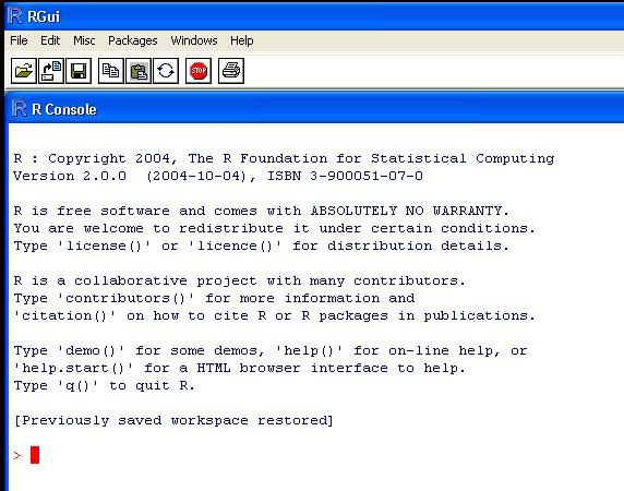
1.2 Use of an Editor Script Window
The screen snapshot in Figure2 shows a script file window. This allows input to R of statements from a file
that has been set up in advance, or that have been typed or copied into the window. To get a script file window,
go to the File menu. If a new blank window is required, click on New script. To load an existing file, click on
Open script…; you will be asked for the name of a file whose contents are then displayed in the window. In
Figure 2 the file was firstSteps.R.
Highlight the commands that are intended for input to R. Click on the `Run line or selection’ icon, which is the
middle icon of the script file editor toolbar in Figs. 2 and 3, to send commands to R.
Fig. 2: The
focus is on an
R display file
window, with
the console
window in the
background.
Fig. 3: This shows the five icons that appear when the focus
is on a script file window. The icons are, starting from the
left:
Open script, Save script, Run line or selection, Return focus
to console, and Print. The text in a script file window can be
edited, or new text added. Display file windows, which have
a somewhat similar set of icons but do not allow editing, are
another possibility.
Under Unix, the standard form of input is the command line interface. Under both Microsoft Windows and
Linux (or Unix), a further possibility is to run R from within the emacs editor4. Under Microsoft Windows,
4
This requires emacs, and ESS which runs under emacs. Both are free. Look under Software|Other on the CRAN page.5
attractive options are to use either the R-WinEdt utility that is designed for use with the shareware WinEdt
editor, or to use the free tinn-R editor5.
1.3 A Short R Session
We will read into R a file that holds population figures for Australian states and territories, and total population,
at various times since 1917, then using this file to create a graph. The data in the file are:
Year NSW Vic. Qld SA WA Tas. NT ACT Aust.
1917 1904 1409 683 440 306 193 5 3 4941
1927 2402 1727 873 565 392 211 4 8 6182
1937 2693 1853 993 589 457 233 6 11 6836
1947 2985 2055 1106 646 502 257 11 17 7579
1957 3625 2656 1413 873 688 326 21 38 9640
1967 4295 3274 1700 1110 879 375 62 103 11799
1977 5002 3837 2130 1286 1204 415 104 214 14192
1987 5617 4210 2675 1393 1496 449 158 265 16264
1997 6274 4605 3401 1480 1798 474 187 310 18532
The following reads in the data from the file austpop.txt on a disk in drive d:
> austpop6
A simple way to get the plot is:
> plot(ACT ~ Year, data=austpop, pch=16) # For the DAAG version, replace ‘Year’ by ‘year’
The option pch=16 sets the plotting character to a solid black dot.
This plot can be improved greatly. We can specify more informative axis labels, change size of the text and of
the plotting symbol, and so on.
1.3.1 Entry of Data at the Command Line
A data frame is a rectangular array of columns of data. Here we will have two columns, and both columns will
be numeric. The following data gives, for each amount by which an elastic band is stretched over the end of a
ruler, the distance that the band moved when released:
stretch 46 54 48 50 44 42 52
distance 148 182 173 166 109 141 166
The function data.frame() can be used to input these (or other) data directly at the command line. We will
give the data frame the name elasticband:
elasticband7
1.3.4 Options for plot() and allied functions
The function plot() and related functions accept parameters that control the plotting symbol, and the size and
colour of the plotting symbol. Details will be given in Section 3.3.
1.4 Further Notational Details
As noted earlier, the command line prompt is
>
R commands (expressions) are typed following this prompt6.
There is also a continuation prompt, used when, following a carriage return, the command is still not complete.
By default, the continuation prompt is
+
In these notes, we often continue commands over more than one line, but omit the + that will appear on the
commands window if the command is typed in as we show it.
For the names of R objects or commands, case is significant. Thus Austpop is different from austpop. For
file names however, the Microsoft Windows conventions apply, and case does not distinguish file names. On
Unix systems letters that have a different case are treated as different.
Anything that follows a # on the command line is taken as comment and ignored by R.
Note: Recall that, in order to quit from the R session we had to type q(). This is because q is a function.
Typing q on its own, without the parentheses, displays the text of the function on the screen. Try it!
1.5 On-line Help
To get a help window (under R for Windows) with a list of help topics, type:
> help()
In R for Windows, an alternative is to click on the help menu item, and then use key words to do a search. To
get help on a specific R function, e.g. plot(), type in
> help(plot)
The two search functions help.search() and apropos() can be a huge help in finding what one wants.
Examples of their use are:
> help.search("matrix")
(This lists all functions whose help pages have a title or alias in which the text string
“matrix” appears.)
> apropos(“matrix”)
(This lists all function names that include the text “matrix”.)
The function help.start() opens a browser window that gives access to the full range of documentation for
syntax, packages and functions.
Experimentation often helps clarify the precise action of an R function.
1.6 The Loading or Attaching of Datasets
The recommended way to access datasets that are supplied for use with these notes is to attach the file
usingR.RData., available from the author's web page. Place this file in the working directory and,
from within the R session, type:
> attach("usingR.RData")
Files that are mentioned in these notes, and that are not supplied with R (e.g., from the datasets or
MASS packages) should then be available without need for any further action.
6
Multiple commands may appear on the one line, with the semicolon (;) as the separator.8
Users can also load (use load()) or attach (use attach()) specific files. These have a similar
effect, the difference being that with attach() datasets are loaded into memory only when required
for use.
Distinguish between the attaching of image files and the attaching of data frames. The attaching of
data frames will be discussed later in these notes.
1.7 Exercises
1. In the data frame elasticband from section 1.3.1, plot distance against stretch.
2. The following ten observations, taken during the years 1970-79, are on October snow cover for Eurasia.
(Snow cover is in millions of square kilometers):
year snow.cover
1970 6.5
1971 12.0
1972 14.9
1973 10.0
1974 10.7
1975 7.9
1976 21.9
1977 12.5
1978 14.5
1979 9.2
i. Enter the data into R. [Section 1.3.1 showed one way to do this. To save keystrokes, enter the successive
years as 1970:1979]
ii. Plot snow.cover versus year.
iii Use the hist() command to plot a histogram of the snow cover values.
iv. Repeat ii and iii after taking logarithms of snow cover.
3. Input the following data, on damage that had occurred in space shuttle launches prior to the disastrous launch
of Jan 28 1986. These are the data, for 6 launches out of 24, that were included in the pre-launch charts that
were used in deciding whether to proceed with the launch. (Data for the 23 launches where information is
available is in the data set orings, from the DAAG package.)
Temperature Erosion Blowby Total
(F) incidents incidents incidents
53 3 2 5
57 1 0 1
63 1 0 1
70 1 0 1
70 1 0 1
75 0 2 1
Enter these data into a data frame, with (for example) column names temperature, erosion, blowby and
total. (Refer back to Section 1.3.1). Plot total incidents against temperature.9
2. An Overview of R
2.1 The Uses of R
2.1.1 R may be used as a calculator.
R evaluates and prints out the result of any expression that one types in at the command line in the console
window. Expressions are typed following the prompt (>) on the screen. The result, if any, appears on
subsequent lines
> 2+2
[1] 4
> sqrt(10)
[1] 3.162278
> 2*3*4*5
[1] 120
> 1000*(1+0.075)^5 - 1000 # Interest on $1000, compounded annually
[1] 435.6293
> # at 7.5% p.a. for five years
> pi # R knows about pi
[1] 3.141593
> 2*pi*6378 #Circumference of Earth at Equator, in km; radius is 6378 km
[1] 40074.16
> sin(c(30,60,90)*pi/180) # Convert angles to radians, then take sin()
[1] 0.5000000 0.8660254 1.0000000
2.1.2 R will provide numerical or graphical summaries of data
A special class of object, called a data frame, stores rectangular arrays in which the columns may be vectors of
numbers or factors or text strings. Data frames are central to the way that all the more recent R routines process
data. For now, think of data frames as matrices, where the rows are observations and the columns are variables.
As a first example, consider the data frame hills that accompanies these notes7. This has three columns
(variables), with the names distance, climb, and time. Typing in summary(hills)gives summary
information on these variables. There is one column for each variable, thus:
> load("hills.Rdata") # Assumes hills.Rdata is in the working directory
> summary(hills)
distance climb time
Min.: 2.000 Min.: 300 Min.: 15.95
1st Qu.: 4.500 1st Qu.: 725 1st Qu.: 28.00
Median: 6.000 Median:1000 Median: 39.75
Mean: 7.529 Mean:1815 Mean: 57.88
3rd Qu.: 8.000 3rd Qu.:2200 3rd Qu.: 68.62
Max.:28.000 Max.:7500 Max.:204.60
We may for example require information on ranges of variables. Thus the range of distances (first column) is
from 2 miles to 28 miles, while the range of times (third column) is from 15.95 (minutes) to 204.6 minutes.
We will discuss graphical summaries in the next section.
7
There are also versions in the DAAG package and in the Venables and Ripley MASS package.10
2.1.3 R has extensive graphical abilities
The main R graphics function is plot(). In addition to plot() there are functions for adding points and lines
to existing graphs, for placing text at specified positions, for specifying tick marks and tick labels, for labelling
axes, and so on.
There are various other alternative helpful forms of graphical summary. A helpful graphical summary for the
hills data frame is the scatterplot matrix, shown in Figure 5. For this, type:
> pairs(hills)
Figure 5: Scatterplot matrix for the Scottish hill race data
2.1.4 R will handle a variety of specific analyses
The examples that will be given are correlation and regression.
Correlation:
We calculate the correlation matrix for the hills data:
> options(digits=3)
> cor(hills)
distance climb time
distance 1.000 0.652 0.920
climb 0.652 1.000 0.805
time 0.920 0.805 1.000
Suppose we wish to calculate logarithms, and then calculate correlations. We can do all this in one step, thus:
> cor(log(hills))
distance climb time
distance 1.00 0.700 0.890
climb 0.70 1.000 0.724
time 0.89 0.724 1.000
Unfortunately R was not clever enough to relabel distance as log(distance), climb as log(climb), and time as
log(time). Notice that the correlations between time and distance, and between time and climb, have reduced.
Why has this happened?
Straight Line Regression:
Here is a straight line regression calculation. The data are stored in the data frame elasticband (DAAG
package). The variable names are the names of columns in that data frame. The formula that is supplied to the
lm() command asks for the regression of distance travelled by the elastic band (distance) on the amount by
which it is stretched (stretch).11
> plot(distance ~ stretch,data=elasticband, pch=16)
> elastic.lm lm(distance ~stretch,data=elasticband)
Call:
lm(formula = distance ~ stretch, data = elasticband)
Coefficients:
(Intercept) stretch
-63.571 4.554
More complete information is available by typing
> summary(lm(distance~stretch,data=elasticband))
Try it!
2.1.5 R is an Interactive Programming Language
We calculate the Fahrenheit temperatures that correspond to Celsius temperatures 25, 26, …, 30:
> celsius fahrenheit conversion print(conversion)
Celsius Fahrenheit
1 25 77.0
2 26 78.8
3 27 80.6
4 28 82.4
5 29 84.2
6 30 86.0
2.2 R Objects
All R entities, including functions and data structures, exist as objects. They can all be operated on as data.
Type in ls() to see the names of all objects in your workspace. An alternative to ls() is objects(). In both
cases there is provision to specify a particular pattern, e.g. starting with the letter `p’8.
Typing the name of an object causes the printing of its contents. Try typing q, mean, etc.
In a long session, it makes sense to save the contents of the working directory from time to time. It is also
possible to save individual objects, or collections of objects into a named image file. Some possibilities are:
save.image() # Save contents of workspace, into the file .RData
save.image(file="archive.RData") # Save into the file archive.RData
save(celsius, fahrenheit, file="tempscales.RData")
Image files, from the working directory or (with the path specified) from another directory, can be attached, thus
making objects in the file available on request. For example
attach("tempscales.RData")
ls(pos=2) # Check the contents of the file that has been attached
The parameter pos gives the position on the search list. (The search list is discussed later in this chapter, in
Section 2.9.)
Important: On quitting, R offers the option of saving the workspace image, by default in the file .RData in the
working directory. This allows the retention, for use in the next session in the same workspace, any objects that
were created in the current session. Careful housekeeping may be needed to distinguish between objects that are
8
Type in help(ls) and help(grep) to get details. The pattern matching conventions are those used for grep(),
which is modelled on the Unix grep command.You can also read