Scaling Auctions as Insurance: A Case Study in Infrastructure Procurement
←
→
Page content transcription
If your browser does not render page correctly, please read the page content below
Scaling Auctions as Insurance: A Case Study in
                  Infrastructure Procurement

                                              ∗                                     †
                    Valentin Bolotnyy                  Shoshana Vasserman

                                          February 2021

                                               Abstract

           Most U.S. government spending on highways and bridges is done through “scaling”
       procurement auctions, in which private construction firms submit unit price bids for
       each piece of material required to complete a project. Using data on bridge maintenance
       projects undertaken by the Massachusetts Department of Transportation (MassDOT),
       we present evidence that firm bidding behavior in this context is consistent with op-
       timal skewing under risk aversion: firms limit their risk exposure by placing lower
       unit bids on items with greater uncertainty. We estimate bidders’ risk aversion, the
       risk in each auction, and the distribution of bidders’ private costs. Simulating equilib-
       rium item-level bids under counterfactual settings, we estimate the fraction of project
       spending that is due to risk and evaluate auction mechanisms under consideration by
       policymakers. We find that scaling auctions provide substantial savings relative to
       lump sum auctions and show how our framework can be used to evaluate alternative
       auction designs.

   ∗
     Hoover Institution, Stanford University. Email: vbolotnyy@stanford.edu
   †
     Stanford Graduate School of Business. Email: svass@stanford.edu. This paper was a chapter in our
PhD dissertations. We are indebted to our advisors Ariel Pakes, Elie Tamer, Robin Lee, Edward Glaeser,
Claudia Goldin, Nathaniel Hendren, Lawrence Katz and Andrei Shleifer for their guidance and support, as
well as to Steve Poftak and Jack Moran, Frank Kucharski, Michael McGrath, and Naresh Chetpelly, among
other generous public servants at MassDOT. Their support was invaluable. We are also very grateful to Ali
Yurukoglu, Andrzej Skrzypacz, Paulo Somaini, Susan Athey and Zi Yang Kang for their many insightful
comments and suggestions, and to Cameron Pfiffer, Philip Greengard and Yingbo Ma for the boost that
their help gave to our computational capacity.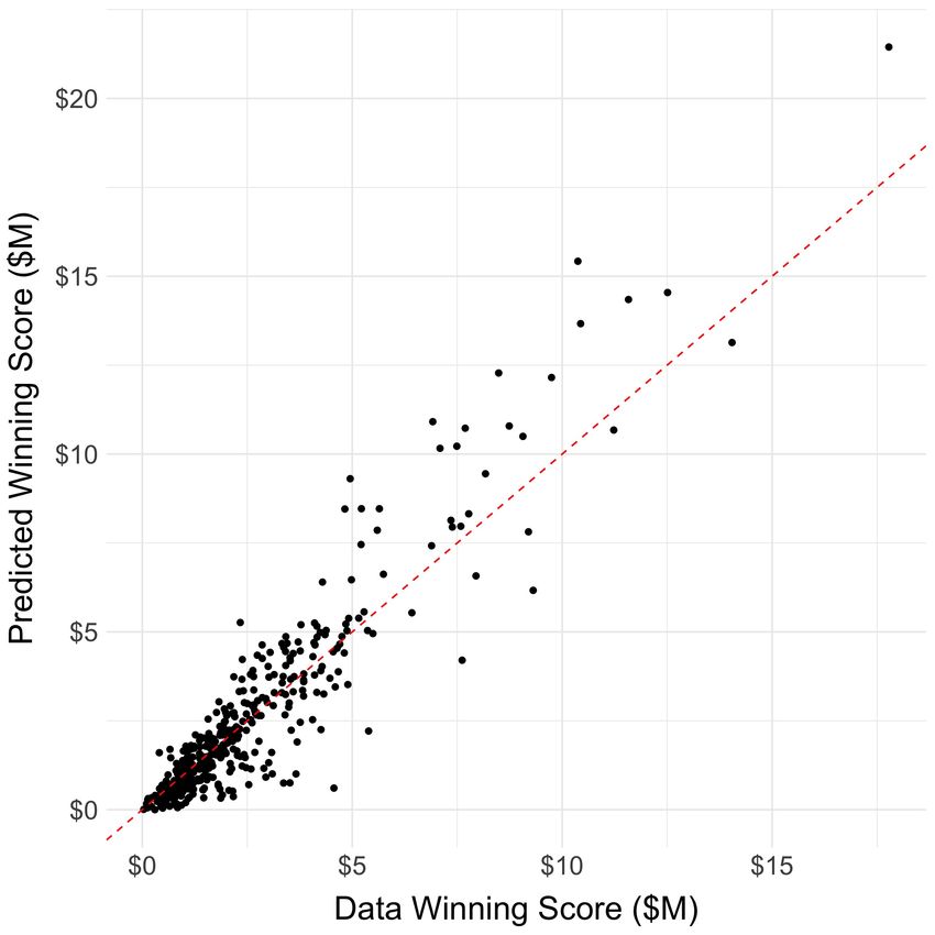
1       Introduction
Infrastructure investment underlies nearly every part of the American economy and consti-
tutes hundreds of billions of dollars in public spending each year.1 However, investments
are often directed into complex projects that experience unexpected changes. Project un-
certainty can be costly to the firms that implement construction—many of whose businesses
are centered on public works—and to the government. The extent of firms’ risk exposure
depends not only on project design, but also on the mechanism used to allocate contracts.
Contracts with lower risk exposure may be more lucrative and thus might invite more com-
petitive bids. As such, risk sharing between firms and the government can play a significant
role in the effectiveness of policies meant to reduce taxpayer expenditures.
    We study the mechanism by which contracts for construction work are allocated by the
Highway and Bridge Division of the Massachusetts Department of Transportation (MassDOT
or “the DOT”). Along with 40 other states, MassDOT uses a scaling auction, whereby
bidders submit unit price bids for each item in a comprehensive list of tasks and materials
required to complete a project. The winning bidder is determined by the lowest sum of unit
bids multiplied by item quantity estimates produced by MassDOT project designers. This
winner is then paid based on the quantities ultimately used in completing the project.
    Scaling auctions thus have several key features. First, they are widespread and common
in public infrastructure procurement. Second, they collect bids over units (that is, tasks and
materials) that are standardized and comparable across auctions. Third, they implement a
partial sharing of risk between the government and private contractors.
    To study auction design in this setting, we specify and estimate a model of bidding in
scaling auctions with risk averse bidders. Our model characterizes equilibrium bids in two
separable steps: an “outer” condition that ensures that a bidder’s score—the weighted sum
of unit bids that is used to determine the winner of the auction—is optimally competitive
with respect to the opposing bidders, and an “inner” condition that ensures that the unit
bids chosen to sum up to the equilibrium score maximize the expected utility of winning.
In effect, the “inner” condition constitutes a portfolio optimization problem for bidders.
Equilibrium unit bids distribute a bidder’s score across different items, trading off higher
expected profits from high bids on items predicted to overrun against higher risk from low
bids on other items.
    The separability of the “inner” and “outer” problems yields a useful property: given an
observation of a bidder’s equilibrium score, her equilibrium unit bids are fully specified by
the characterization of her (“inner”) portfolio problem. This allows us to both interpret
    According to the CBO, infrastructure spending accounts for roughly $416B or 2.4% of GDP annually
    1

across federal, state and local levels. Of this, $165B—40%—is spent on highways and bridges alone.

                                                 1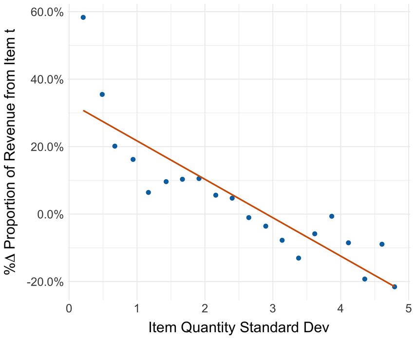
reduced form patterns of risk-averse bidding behavior and to estimate the primitives that
rationalize the unit bids observed in our data, without specifying the data generating process
for the scores themselves.
    Using a detailed data set obtained through a partnership with MassDOT, we establish
the patterns of bidding behavior that motivate our approach. For each auction in our study,
we observe the full set of items involved in construction, along with ex-ante estimates and
ex-post realizations of the quantity of each item, a DOT estimate of the market unit rate for
the item, and the unit price bid that each bidder who participated in the auction submitted.
As in prior work on scaling auctions, we show that contractors skew their bids, placing high
unit bids on items they believe will overrun the DOT quantity estimates and low unit bids
on items they believe will under-run. This suggests that contractors are generally able to
predict the direction of ex-post changes to project specifications, and bid so as to increase
their ex-post earnings.
    Furthermore, our data suggest that contractors are risk averse. As noted in Athey and
Levin (2001), risk neutral bidders would be predicted to submit “penny” bids—unit bids of
essentially zero—on all but the items that are predicted to overrun by the largest amount.
By contrast, the vast majority of unit bids observed in our data are interior (that is, non-
extremal), even though no significant penalty for penny bidding has ever been exercised.
We show that while contractors bid higher on items predicted to overrun, holding all else
fixed, they also bid lower on items that are more uncertain. This suggests that contractors
optimize not only with respect to expected profits, but also with respect to the risk that any
given expectation will turn out to be wrong.
    Risk aversion, combined with inherent project risk, has significant implications for DOT
spending, as well as for the efficacy of policies to reduce it. Risk averse bidders internalize
a utility cost from uncertainty, and require higher overall bids in order to insure themselves
sufficiently to be willing to participate. As such, auction rules that decrease bidders’ exposure
to significant losses can be effective toward lowering overall bids, and subsequently lowering
DOT payments to the winning bidder.
    In order to gauge the level of risk and risk aversion in our data, we estimate a structural
model of uncertainty and optimal bidding. In the first stage of our estimation procedure, we
use the history of predicted and realized item quantities to fit a model of bidder uncertainty
over item quantity realizations. In the second stage, we construct a Generalized Method
of Moments (GMM) estimator for bidders’ risk aversion, as well as their private costs, in
each project. Our estimator relies only on predictions of optimal unit bids at the auction-
bidder-item level, evaluated from each bidder’s portfolio problem under the constraint of her
observed score. As such, our identification strategy leverages granular variation in project

                                               2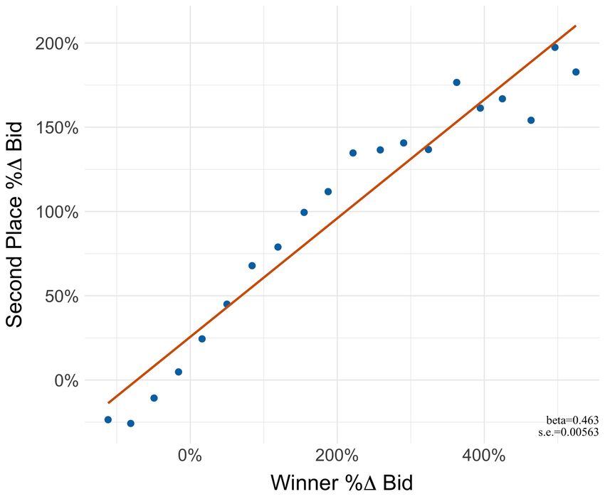
composition (e.g., which items are needed, at what market rate, and in what quantities),
in addition to more standard project characteristics such as the identity of the designing
engineer. As our predictions of optimal bids capture the bidders’ competitive considerations
entirely through the score—which is taken as data—our estimation approach does not re-
quire strong assumptions about bidders’ beliefs about their opponents, nor does it require
exogenous variation in the composition of bidders across auctions.
    We use our structural estimates to evaluate not only the cost of uncertainty to the DOT,
but also the performance of scaling auctions relative to alternatives used in other procure-
ment settings. Using an independent private values framework, we simulate the equilibrium
outcomes under a counterfactual setting in which uncertainty about item quantities is re-
duced to zero. When bidder predictions are unaffected—the only change is that uncertainty
about these predictions is eliminated—we find that DOT spending decreases by 13.5% for
the median auction. This suggests that project uncertainty contributes to a substantial risk
premium.
    However, scaling auctions perform quite well given the level of uncertainty in these
projects. The most common alternative type of procurement mechanism is a lump sum
auction, in which bidders commit to a total payment for the project at the time of the auc-
tion and are liable for all implementation costs afterward. Lump sum auctions require less
planning by the DOT, and they incentivize bidders to be economical when they can be. But
for projects that are highly standardized and monitored—such the bridge projects in our
data—lump sum auctions primarily shift risk from the DOT onto the risk-averse bidders.
Seen in this light, scaling auctions provide a powerful lever for the DOT to lower its costs:
not only do scaling auctions provide insurance by reimbursing bidders for every item that
is ultimately used, but they also allow bidders to hedge their risks through portfolio opti-
mization. In our simulations, we find that moving from the scaling format to a lump sum
format would increase DOT spending by 69% for the median auction, although the increase
is much lower if ex-post renegotiation is possible.
    Given these results, we ask whether scaling auctions can be further improved through
a policy that might reasonably be considered by the DOT. The first answer is negative.
Although we find a substantial risk premium from eliminating uncertainty holding everything
else fixed, a policy to reduce uncertainty—through training or directives, for instance—
may not be very effective at reducing costs in practice. Uncertainty in our data is fairly
symmetric: under-runs and over-runs both occur frequently, both in quantities and in DOT
spending. As such, when we compare the no-uncertainty counterfactual against the status-
quo, DOT savings in the median auction are reduced to only 0.28%, with losses at the
25th percentile. This is because eliminating uncertainty gives bidders access to the exact

                                             3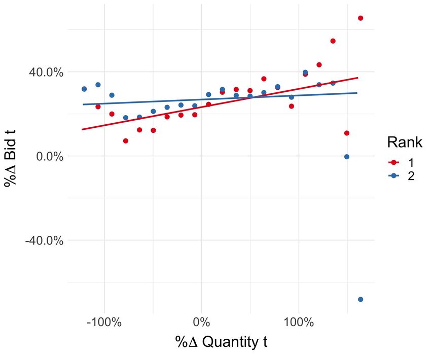
quantities that will ultimately be used, allowing them to avoid making “mistakes” (from
an ex-post perspective) that had benefited the DOT under uncertainty. In some cases, this
difference in predictions dominates the elimination of the risk premium. Thus, although we
find that reducing uncertainty is beneficial to the DOT on net, it may not hold up to scrutiny
when practical considerations are accounted for.
    However, an alternative proposal that was raised by MassDOT in 2017—but was ulti-
mately defeated—may be worth considering. We examine a policy in which each item is given
a strictly positive unit reservation price. When bidders maximize their portfolios of bids un-
constrained, they balance maximizing their expected profits against minimizing their risk.
This generally does not result in the risk-minimizing spread. A minimum reservation price
forces bidders to bid higher on items that they are willing to be effectively uncompensated
for. While this moves bidders away from their optimal portfolio, it also lowers the risk that
they undertake. Furthermore, as all bidders are subject to the same constraint, competition
entails that the distribution of scores does not change substantially in equilibrium, and so
bidders are forced to lower their bids for items that they would strongly overbid otherwise.
As a result, the risk premium paid by the DOT decreases endogenously. Considering a unit
reservation price of 25% of each item’s market rate, we find that the risk premium decreases
by a fifth. A policy of this sort may thus present a cost-effective way to improve on the
status quo.

2    Related Literature
Strategic bid skewing in scaling auctions has been documented in various contexts where
bidders may be better informed than the auctioneer. Studying US timber auctions, Athey
and Levin (2001) first established that positive correlations between (dollar) over-bids and
(unit) over-runs in auction data could be interpreted as evidence that bidders are able to
predict which components of their bids will overrun. Bajari, Houghton, and Tadelis (2014)
made a similar observation in the context of highway paving procurement auctions in Cali-
fornia. However, neither paper evaluates the welfare impact of bid-skewing or the underlying
uncertainty that causes it.
    Bidders who are risk-neutral, such as in the model proposed by Bajari et al. (2014), would
be predicted to skew “completely”—that is, bid very high on one component of the project
and zero on all the others—unless they face an additional incentive not to do so. Moreover,
absent such an incentive, there is no welfare cost to skewing whatsoever: were the government
to perfectly predict quantities such that there are no over-runs, the ultimate payment to the
winning bidder would be the same. Bajari et al. (2014) accounts for the lack of complete

                                              4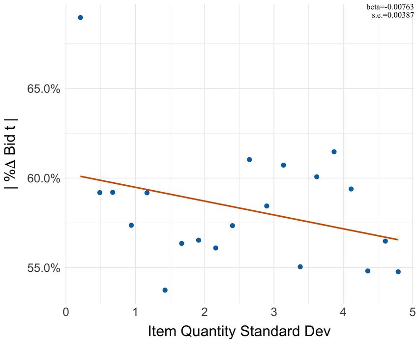
skewing in their data by imposing a penalty on unit bids that increases in the distance
between the bid and the government’s unit cost estimate, as well as the distance between
the ex-ante unit quantity estimate and the ex-post realization of that quantity. While this
enables Bajari et al. (2014) to structurally estimate average adaptation cost multipliers and
calibrate the cost of ex-post renegotiation, the penalty function coefficient is found to be
insignificantly different from zero, and no bidder-specific types or counterfactual strategies
are estimated.
    As in Athey and Levin (2001), our paper argues that the absence of complete skewing
is primarily driven by risk aversion. Our model of risk averse bidding predicts that unit
bids will be skewed both as a function of bidders’ predictions of ex-post quantities and the
amount of uncertainty in each prediction. The heart of our paper rests in the resulting
portfolio optimization problem, which determines the spread of unit bids for each score that
a bidder submits, and consequently, both the bidder’s private value for winning the auction
and the government’s ex-post payment to the bidder if she wins—both of which differ from
the score itself.
    Our portfolio characterization of bid skewing has several key implications for the anal-
ysis of scaling auctions. First, it allows us to construct reduced form correlation tests for
risk aversion: much as a positive correlation between over-bids and over-runs is evidence of
bidder information, a negative correlation between absolute markups and component-level
uncertainty is indicative of risk aversion. Second, it provides a novel channel for identi-
fication of bidder and auction-level model parameters. Our identification strategy differs
from the canonical approaches of Guerre, Perrigne, and Vuong (2009), Campo, Guerre, Per-
rigne, and Vuong (2011) and Campo (2012). Like these papers, we require functional form
assumptions such as the CARA utility function. However, whereas their approaches rely
on the optimality of single-dimensional bids with respect to the probability of beating out
other bidders—analogous to the first order condition characterizing the optimal score in our
model—our approach uses the optimality of the composition of unit bids to maximize the
value of executing a contract conditional on each bidder’s score.
    This has important implications for the assumptions about equilibrium play that are
required. The Campo and GPV approaches require bids to be interpreted as equilibrium
outcomes of an explicit competitive bidding game—whether a symmetric IPV game or an
asymmetric affiliated values game. By contrast, our identification approach is agnostic to the
competitive conditions under which each bidder’s score is chosen. Subject to comparatively
weak conditions that guarantee the separability of the deterministic portfolio-optimization
problem from the equilibrium problem of choosing a score for each bidder, our identifi-
cation strategy is robust to a number of alternative settings, dynamic considerations and

                                              5
collusion. This does not mean that we are impervious to the non-identification results de-
tailed in Guerre et al. (2009): we still require a parametric (or potentially, semi-parametric)
characterization of bidders’ utility and exogenous variation in the distribution of contract
values across auctions. However, the particular assumptions needed are different: instead
of assumptions about bidders’ beliefs about each other, we use assumptions about bidders’
beliefs about project characteristics. This set of assumptions may be preferable in a highly
standardized infrastructure procurement setting such as ours, where historical information
is publicly available and bidders are often industry veterans, but where inherent uncertainty
about the underlying physical conditions at each project site is high.
Finally, our portfolio approach facilitates counterfactual analyses of alternative auction
rules. Because bidders are not paid the score that they compete with—but rather a linear
transformation of their unit bids—a prediction of counterfactual scores that does not model
the relationship between scores and unit bids would be insufficient to generate predictions
for government cost or welfare. Using our model, we evaluate policies to reduce uncertainty
regarding item quantities, to pre-commit payments at the time of bidding, and to enforce
minimum unit bids on all items.
Our paper contributes to a substantial literature on the efficiency of infrastructure pro-
curement auctions.2 Closest to us is Luo and Takahashi (2019), a contemporary paper that
studies infrastructure procurement by the Florida DOT. Like us, Luo and Takahashi (2019)
considers risk averse bidders and compares scaling auctions against lump sum auctions.
However, this paper follows a GPV/Campo-style approach for identification and reduces
the project components that receive unit bids (which number 67 for the median auction in
our dataset) into two aggregates—one with bidder-auction-specific variation and one with
a bidder-auction-specific mean—for estimation. As such, while Luo and Takahashi (2019)
offers novel evidence of risk aversion and the costliness of lump sum auctions in settings with
high uncertainty, we view our analyses as complementary in methodology and contribution.
More generally, our paper builds on a rich literature on scoring auctions. While the the-
oretical results for risk-neutral bidders in Che (1993) and Asker and Cantillon (2008) do not
apply to our model directly, the separability of equilibrium bidding into an ”outer” score-
setting stage and an ”inner” portfolio-maximizing stage in our model is closely related to the
separability of quality provision and bidding. Our paper also relates to the theoretical liter-
ature on optimal mechanism design. While we focus on “practical” mechanisms—ones that
do not require knowledge of the bidder type distribution, for instance—it is possible to char-
acterize the theoretically optimal mechanism for our setting by applying the characterization
in Maskin and Riley (1984) and Matthews (1987) to our framework.
2
See for instance, Lewis and Bajari (2011) and Krasnokutskaya and Seim (2011).
63 Scaling Auctions with MassDOT
Like most other states, Massachusetts manages the construction and maintenance for its
highways and bridges through its Department of Transportation. In order to develop a new
project, MassDOT engineers assemble a detailed specification of what the project will entail.
This includes an itemized list of every task and material (item) that is necessary to complete
the project, along with estimates for the quantity with which it will be needed, and a market
unit rate for its cost. The itemized list of quantities is then advertised to prospective bidders.
In order to participate in an auction for a given project, a contractor must first be pre-
qualified by MassDOT. Pre-qualification entails that the contractor is able to complete the
work required, given their staff and equipment. Notably, it generally does not depend on
past performance. In order to submit a bid, a contractor posts a unit price for each of
the items specified by MassDOT. Since April 2011, all bids have been processed through
an online platform, Bid Express, which is also used by 41 other state DOTs. All bids are
private until the completion of the auction.
Once an auction is complete, each contractor is given a score, computed by the sum of
the product of each item’s estimated quantity and the contractor’s unit-price bid for it. The
bidder with the lowest score is then awarded a contract to execute the project in full. In the
process of construction, it is common for items to be used in quantities that deviate from
MassDOT specifications. All changes, however, must be approved by an on-site MassDOT
manager. The winning contractor is ultimately paid the sum of her unit price bid multiplied
by the actual quantity of each item used. Unit prices are almost never renegotiated. However,
there is a mechanical price adjustment on certain commodities such as steel and gasoline if
their market prices fluctuate beyond a predefined threshold (typically 5%).3
MassDOT reserves the right to reject bids that are heavily skewed. However, this has
never been successfully enforced and most bids violate the condition that should trigger
rejection.4 MassDOT has entertained other proposals to curtail bid skewing, such as a 2017
push to require a minimum unit price on each item. However, this proposal was defeated
after bidder protests.
4 Data and Reduced Form Results
Our data come from MassDOT and cover highway and bridge construction and maintenance
projects undertaken by the state from 1998 to 2015. We work with projects for which
MassDOT has digital records on 1) identities of the winning and losing bidders; 2) bids for
3
See https://www.mass.gov/service-details/massdot-special-provisions for details.
4
See Section B in the Online Appendix for a detailed discussion.
7the winning and losing bidders; and 3) data on the actual quantities used for each item.
2,513 projects meet these criteria, 440 of which are related to bridge work. We focus on
bridge projects alone for this paper, as these projects are particularly prone to item quantity
adjustments.
All bidders who participate in auctions for these projects are able to see, ex-post, how
everyone bid on each item. In addition, all contractors have access to summary statistics on
past bids for each item, across time and location. Officially, all interested bidders find out
about the specifications and expectations of each project at the same time, when the project
is advertised (a short while before it opens up for bidding). Only those contractors who
have been pre-qualified at the beginning of the year to do the work required by the project
can bid on the project. Thus, contractors do not have a say in project designs, which are
furnished either in-house by MassDOT or by an outside consultant.
Once a winning bidder is selected, project management moves under the purview of an
engineer working in one of six MassDOT districts around the state. This Project Manager
assigns a Resident Engineer to monitor work on a particular project out in the field and to
be the first to decide whether to approve or reject under-runs, over-runs, and Extra Work
Orders (EWOs). The full approval process of changes to the initial project design involves
several layers of review. Under-runs and over-runs, as the DOT defines them and as we will
define them here, apply to the items specified in the initial project design and refer to the
difference between actual item quantities used and the estimated item quantities. EWOs
refer to work done outside of the scope of the initial contract design and are most often
negotiated as lump sum payments from the DOT to the contractor. For the purposes of our
discussion and analyses, we will focus on under-runs and over-runs in bridge construction
and maintenance projects.
Statistic Mean St. Dev. Pctl(25) Median Pctl(75)
Project Length (Estimated) 1.53 years 0.89 years 0.88 years 1.48 years 2.01 years
Project Value (DOT Estimate) $2.72 million $3.89 million $981,281 $1.79 million $3.3 million
# Bidders 6.55 3.04 4 6 9
# Types of Items 67.80 36.64 37 67 92
Net Over-Cost (DOT Quantities) −$286,245 $2.12 million −$480,487 −$119,950 $167,933
Net Over-Cost (Ex-Post Quantities) −$26,990 $1.36 million −$208,554 $15,653 $275,219
Extra Work Orders $298,796 $295,173 $78,775 $195,068 $431,188
Table 1: Summary Statistics
Table 1 provides summary statistics for the bridge projects in our data set. We measure
the extent to which MassDOT overpays the projected project cost in two ways. First,
we consider the difference between what the DOT ultimately pays the winning bidder and
the DOT’s initial estimate of what it will pay at the conclusion of the auction. Summary
8statistics for this measure are presented in the “Net Over-Cost (DOT Quantities)” row of
Table 1.
While it seems as though the DOT is saving money on net, this is a misrepresentation
of the costs of bid skewing. The initial estimate—which uses the DOT’s ex-ante quantity
estimates and corresponds to the winning bidder’s score in our model—is not necessarily
representative of the payments that the bidder expects upon winning. Sophisticated bidders
anticipate changes from the initial DOT estimates, and bid accordingly to maximize their
ex-post payments. As such, a more appropriate metric is to compare the amount that was
ultimately spent in each project against the dot product of the DOT’s unit cost estimates and
the actual quantities used. This is presented in the “Net Over-Cost (Ex-Post Quantities)”
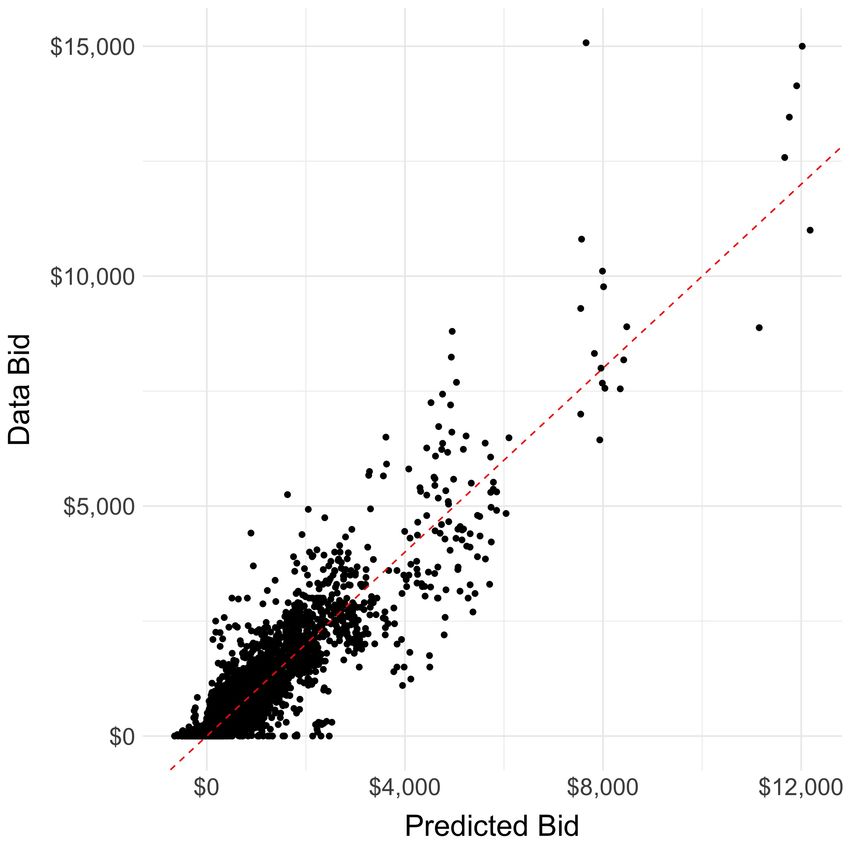
row of Table 1. The median over-payment by this metric is about $15,000, but the 25th
and 75th percentiles are about -$210,000 and $275,000. Figure 1 shows the spread of over-
payment across projects. As we will show in our counterfactual section, the distribution of
over-payment corresponds to the potential savings from the elimination of risk.
Figure 1: Net Over-Cost (Ex-Post Quantities) Across Bridge Projects
Bidder Characteristics There are 2,883 unique project-bidder pairs (i.e., total bids sub-
mitted) across the 440 projects that were auctioned off. There are 116 unique firms that
participate, albeit to different degrees. We divide them into two groups: ‘common’ firms,
which participate in at least 30 auctions within our data set, and ‘rare firms‘, which partic-
ipate in fewer than 30 auctions. We retain individual identifiers for each of the 24 common
firms, but group the 92 rare firms together for purposes of estimation. Common firms con-
stitute 2,263 (78%) of total bids submitted and 351 (80%) of auction victories.
Although there is little publicly available financial information about them, the firms in
our data are by and large relatively small, private, family-owned businesses. Table 2 presents
summary statistics of the two firm groups. The mean (median) common firm submitted bids
to 94.29 (63) auctions and won 14.62 (10) of them. The mean total bid (or score) is about $2.8
9Common Firm Rare Firm
Number of Firms 24 92
Total Number of Bids Submitted 2263 620
Mean Number of Bids Submitted Per Firm 94.29 6.74
Median Number of Bids Submitted Per Firm 63.0 2.5
Total Number of Wins 351 89
Mean Number of Wins Per Firm 14.62 0.97
Median Number of Wins Per Firm 10 0
Mean Bid Submitted $2,774,941 $4,535,310
Mean Ex-Post Cost of Bid $2,608,921 $4,159,949
Mean Ex-Post Over-run of Bid 9.7% 21.97%
Percent of Bids on Projects in the Same District 28.19% 15.95%
Percent of Bids by Revenue Dominant Firms 51.67% 11.80%
Mean Specialization 24.44 2.51
Mean Capacity 10.38 2.75
Mean Utilization Ratio 53.05 25.50
Table 2: Comparison of Firms Participating indistinct project types, according to DOT taxonomy: Bridge Reconstruction/Rehabilitation,
Bridge Replacement, and Structures Maintenance. The mean specialization of a common
firm is 24.44%, while the mean specialization of a rare firm is 2.51%. As projects have
varying sizes, we compute a measure of specialization in terms of project revenue as well.
We define a revenue-dominant firm (within a project-type) as a firm that has been awarded
more than 1% of the total money spent by the DOT across projects of that project type.
Among common firms, 51.67% of bids submitted were by firms that were revenue dominant
in the relevant project type; among rare firms, the proportion of bids by revenue dominant
firms is 11.8%.
A third factor of competitiveness is each firm’s capacity—the maximum number of DOT
projects that the firm has ever had open while bidding on another project—and a fourth
factor is its utilization—the share of the firm’s capacity that is filled when it is bidding on the
current project. We measure capacity and utilization with respect to all MassDOT projects
recorded in our data—not just bridge projects. The mean capacity is 10.38 projects among
common firms and 2.75 projects among rare firms. This suggests that rare firms generally
have less business with the DOT, either because they are smaller in size, or because the
DOT constitutes a smaller portion of their operations. The mean utilization ratio, however,
is 53.05% for common firms and 25.5% for rare firms. This suggests that firms in our data
are likely to have ongoing business with the DOT at the time of bidding and are likely to
have spare capacity during adjacent auctions that they did not participate in. While we do
not model the dynamic considerations of capacity constraints directly, we find our measure
of capacity to be a useful metric of the extent of a firm’s dealings with the DOT, as well as
its size.
Quantity Estimates and Uncertainty As we discuss in Section 8, scaling auctions
mitigate DOT costs by enabling risk-averse bidders to insure themselves against uncertainty
about the item quantities that will ultimately be used for each project. The welfare benefit is
particularly strong if the uncertainty regarding ex-post quantities varies across items within
a project, and especially so if there are a few items that have particularly high variance.
When this is the case, bidders in a scaling auction can greatly reduce the risk that they face
by placing minimal bids on the uncertain items (and higher bids on more predictable items).
Our data set includes records of 2,985 unique items, as per MassDOT’s internal taxonomy.
Spread across 440 projects, these items constitute 29,834 unique item-project pairs. Of the
2,985 unique items, 50% appear in only one project. The 75th, 90th, and 95th percentiles of
unique items by number of appearances in our data are 4, 16, and 45 auctions, respectively.
For each item, in every auction, we observe the quantity with which the DOT predicted it
11would be used at the time of the auction—qte in our model—the quantity with which the item
was ultimately used—qta —and a DOT engineers’ estimate of the market rate for the unit
cost of the item. The DOT quantities are typically inaccurate: 76.7% of item observations
in our data had ex-post quantities that deviated from the DOT estimates.
Figure 2a presents a histogram of the percent quantity over-run across item observations.
The percent quantity over-run is defined as the difference of the ex-post quantity of an item
q a −q e
observation and its DOT quantity estimates, normalized by the DOT estimate: t qe t . In
t
addition to the 23.3% item-project observations in which quantity over-runs are 0%, another
18% involve items that are not used at all (so that the over-run is equal to -100%). The
remaining over-runs are distributed more or less symmetrically around 0%.
The ex-post deviations from DOT quantity estimates result from a number of different
mechanisms. Some deviations arise from standard procedures. For instance, as ex-ante DOT
estimates are used for budgeting purposes, there may be reason for adjusting the quantities
of certain items after the design stage. One example is concrete, which is heavily used, has
quantities that are difficult to predict precisely, and often overruns in our data. It is also
common for the DOT to include certain items that are unlikely to be used at all—just in
case—in order to support its policy of avoiding ex-post renegotiation. Prominent examples
of such items include flashing arrows and illumination for night work. While mechanisms
of this sort are largely systemic, there remains a substantial amount of variation in ex-
post quantities simply due to the inherent uncertainty of construction. A large fraction
of Massachusetts bridges are structurally deficient, making it difficult to ascertain the exact
severity of their condition prior to construction. From our conversations with DOT engineers,
these mechanisms are known symmetrically by all of the bidders. Motivated by profit, bidders
are also generally thought to have better institutional knowledge and quality predictive
software than the DOT.
We document, furthermore, that quantity over-runs vary across observations of the same
item in different auctions. Figure 2b plots the mean percent quantity over-run for each
unique item with at least 2 observations against its standard deviation. While a few items
have standard deviations close to 0, the majority of items have over-run standard deviations
that are as large or larger than the absolute value of their means. That is, the percent
over-run of the majority of unique items varies substantially across observations. While this
is a coarse approximation of the uncertainty that bidders face with regard to each item—it
does not take item or project characteristics into account, for example—it is suggestive of
the scope of risk in each auction.
Reduced Form Evidence for Risk Averse Bid Skewing As in Athey and Levin (2001)
and Bajari et al. (2014), the bids in our data are consistent with a model of similarly in-
12(a) Histogram of the percent quantity over-run (b) Scatterplot of standard deviation vs mean
across item-project pairs. quantity over-run for each unique item.
Figure 2
formed bidders who bid strategically to maximize expected utility. In Figure 3a, we plot
the relationship between quantity over-runs and the percent by which each item was overbid
above the blue book cost estimate. We do this for both the winning bidder and the second
place bidder.5 The binscatter is residualized. In order to obtain it, we first regress percent
over-bid on a range of controls and obtain residuals. We then regress percent over-run on the
same controls and obtain residuals. Finally, to obtain the slope, we regress the residuals from
the first regression on the residuals from the second. Controls include the DOT estimate of
total project cost, the initially stated project length in days, and the number of participating
bidders, as well as fixed effects for: item IDs, the year in which the project was opened for
bidding, the project type, resident engineer, project manager, and project designer. Specifi-
cations that exclude item fixed effects or include an array of additional controls produce very
similar slopes.6 We use a similar procedure for all residualized binscatters in this section.
As Figure 3a demonstrates, there is a significant positive relationship between percent
quantity over-runs and percent over-bids by the winning bidder. A 1% increase in quantity
over-runs corresponds to a 0.086% increase in over-bids on average. Higher bids on over-
5 bt −ct
The percent over-bid of an item is defined as ct × 100, where bt is the bid on item t and ct is the DOT
q a −q e
market rate estimate of item t. The percent quantity over-run is similarly defined as t qe t × 100, where qta
t
is the amount of item t that was ultimately used and qte is the DOT quantity estimate for item t that is used
to calculate bidder scores.
6
For each graph, we truncate observations at the top and bottom 1%. This is done for the purposes of
clarity as outliers can distort the visibility of the general trends.
13running items correspond to higher earnings ex-post. Thus, as higher bids correspond to
items that overran in our data, we conclude that the winning bidder is able to correctly
predict which items will overrun the DOT estimates on averages, and to skew strategically
accordingly.
Furthermore, Figure 3a shows that losing bidders skew their bids in a similar way to
winning bidders. With the exception of a few outlying points, the relationship between over-
bids and over-runs is very similar between the top two bidders: they both overbid on items
that wound up overrunning on average. This suggests that the winning and second place
bidder are similarly able to predict over-runs. In Appendix G, we show that this relationship
for the second-place bidder is even stronger when we restrict our comparison to projects in
which the first two bidders submit similar total scores and thus have similar private costs of
production.
(a) Residualized binscatter of item-level percent (b) Binscatter of item-level percent over-bids by
over-bid by the rank 1 (winning) and rank 2 the rank 2 bidder against the rank 1 (winning)
bidder, against percent quantity over-run. bidder.
Figure 3
While our data suggest that bidders do engage in bid skewing, there is no evidence of
total bid skewing, in which a few items are given very high unit bids and the rest are given
“penny bids”. The average number of unit bids worth $0.10 or less by the winning bidder
is 0.51—or 0.7% of the items in the auction. The average number of unit bids worth $0.50,
$1.00, and $10.00, respectively, is 1.68, 2.85 and 13.91, corresponding to 2.8%, 4.73%, and
23.29% of the items in the auction. This observation is consistent with previous studies of
bidding in scaling auctions. Athey and Levin (2001) argue that the interior bids observed in
their data are suggestive of risk aversion among the bidders. While they acknowledge that
other forces, such as fear of regulatory rebuke, may provide an alternative explanation for
the lack of total bid skewing, they note that risk avoidance was the primary explanation
14given to them in interviews with professionals.
In addition to interior bids, risk aversion has several testable theoretical implications.
Risk averse bidders balance the incentive to bid high on items that are projected to overrun
with an incentive to bid closer to cost on items that are uncertain. As our model in Section 5
shows, bidders with higher costs and higher scores face larger amounts of risk from extremal
bids. As such, they are less willing to skew strongly or bid far below cost on items predicted
to under-run.7
This observation is consistent with the pattern demonstrated in Figure 3a. Here, the
second place bidder—who submitted a higher overall score by definition—generally exhibits
less severe skewing: a 1% increase in quantity over-runs corresponds to only a 0.019% increase
in over-bids on average. Figure 3b, which plots a residualized binscatter of the second place
bidder’s unit bid for each item against the winning bidder’s unit bid for the same item, shows
a similar pattern.8 While the direction of skewing corresponds strongly between the top two
bidders—a higher over-bid by the winning bidder corresponds to a higher over-bid by the
second place bidder as well—the second place bidder’s skewing is more subdued.
The bids in our data also exhibit more direct evidence of risk aversion. We would expect
risk averse bidders to bid lower markups on items that—everything else held fixed—have
higher uncertainty. While we do not see observations of the same item in the same context
with identifiably different uncertainty, we present the following suggestive evidence that such
behavior is occurring.
In Figures 4a and 4b, we plot the relationship between the unit bid for each item in each
auction by the winning bidder, and an estimate of the level of uncertainty regarding the
ex-post quantity of that item (in the context of the particular auction). To calculate the
level of uncertainty for each item, we use the results of our first stage estimation, discussed
in Section 6. For every item, in every auction, our first stage gives us an estimate of the
variance of the error for the best prediction of what the ex-post quantity of that item would
be, given information available at the time of bidding.
In Figure 4a, we plot a residualized binscatter of the winning bidder’s absolute percent
over-bid on each item against the item’s standard deviation—the square root of the estimated
prediction variance. This captures the uncertainty of each item quantity prediction across
auctions in which it may appear with different DOT expectations and project compositions
and characteristics. The relationship is negative, suggesting that holding all else fixed,
bidders bid closer to cost on items with higher variance and thus limit their risk exposure.
7
See Supplemental Appendix A.2 for a worked out example and intuition.
8
Note that the percent over-bids in Figure 3b appear to be substantially larger than those in Figure 3a.
This is because while large over-bids occur in the data, they are relatively rare and so are averaged down in
the percent quantity over-run binning in Figure 3a.
15(a) Residualized binscatter of item-level percent (b) Residualized binscatter of item-level percent
absolute over-bid against the square root of difference in cost contribution against the
estimated item quantity variance. square root of estimated item quantity variance.
Figure 4
Note, however, that this analysis does not directly account for the trade-off between quantity
over-runs and uncertainty. As in Equation (5), a bidder’s certainty equivalent increases in the
predicted quantity of each item, but decreases in the item’s quantity variance. To account
for this trade-off, we consider the following alternative metric for bidding high on an item:
b qa c qe
Pt t a − Pt t e
bp qp ct qp
p p
%∆ Revenue Contribution from t = c qe
× 100
Pt t e
ct qp
p
This is the percentage difference in the proportion of the total revenue earned by the
winning bidder from item t, and the proportion of the DOT’s initial cost estimate that item
t constituted. We take the percent difference between the item’s revenue contribution to the
bidder and its cost contribution to the DOT’s total estimate in order to normalize across
items that inherently play a bigger or smaller role in a project’s total cost. In Figure 4b, we
plot the residualized binscatter of the %∆ Revenue Contribution due to each item against
the item’s quantity standard deviation. The negative relationship here is particularly pro-
nounced, providing further evidence that bidders allocate proportionally less weight in their
expected revenue to items with high variance. Our model of risk averse bidding predicts
exactly this kind of relationship.
165 A Structural Model for Bidding With Risk Aversion
In this section, we present the theoretical framework underlying our empirical exercise. We
first present our baseline model, in which bidders competing in an auction share a common
CARA utility function. We then discuss extensions to CRRA utility and asymmetric risk
aversion types.
5.1 The Baseline Model
A procurement auction consists of N qualified bidders competing for a contract to complete
a single construction project. Each project is characterized by T items, each of which is
ultimately needed in a different quantity. Prior to bidding, bidders observe a DOT estimate
qte for each item t’s quantity, as well as an additional noisy public signal qtb . Although we do
not model this explicitly until Section 6, the public signal should be thought of as a refinement
of qte that incorporates further public information, such as the identity of the designing
engineer and historical trends for similar projects. Upon completion of construction, the
actual quantity qta of each item is realized, independently of which bidder won the auction
and at what price. To summarize, there are three kinds of quantity objects:
• qe = {q1e , . . . , qTe }: DOT estimates based on underlying conditions at the project site
• qb = {q1b , . . . , qTb }: Common refined estimates based on public information
• qa = {q1a , . . . , qTa }: Actual quantities, realized ex-post independently of the auction
In order to participate in the auction, each bidder i must submit a unit bid bi,t for every
item t involved in the auction. Bids are simultaneous and sealed until the conclusion of the
auction. To determine a winner, each bidder i is given a score based on her unit bids and
the DOT quantity estimates: si = Tt=1 bi,t qte . The bidder with the lowest score wins the
P
contract and executes the project in full. Once the project is complete, the winning bidder is
paid her unit bid bi,t for each item t multiplied by the actual quantity of t that was needed,
qta .
Bidder Types The winner of a procurement auction is responsible for securing all of the
items required to complete construction. The majority of these items—such as concrete
and traffic cones—are standard, competitive goods that have a commonly-known market
unit cost ct at the time of the auction. However, bidders differ in their labor, storage and
transportation costs across different projects. To capture this, we assume that bidders differ
along a single-dimensional efficiency multiplier α. That is, for every item t required for a
17project, bidder i faces a unit cost of αi ct , where αi is the bidder’s efficiency type. Each bidder
privately observes her efficiency type prior to bidding. However, it is common knowledge
that efficiency types are drawn independently from a common, publicly known distribution
over a compact subset [α, α] of R+ .
Uncertainty and Risk Aversion Bidder expectations for the quantities with which dif-
ferent items will be needed are noisy to different degrees. For tractability, we assume that
the bidders’ public signal for each item t in our baseline specification is normally distributed
around the actual quantity of t, with an item-specific variance parameter:
qtb = qta + εt , where εt ∼ N (0, σt2 ). (1)
In addition, we assume that bidders are risk averse with a standard CARA utility function
over their earnings from the project and a common constant coefficient of absolute risk
aversion γ:
u(π) = 1 − exp(−γπ). (2)
Bidder Payoffs If a bidder loses the auction, she does not pay or earn anything regardless
of her bid. If bidder i wins the auction with bid vector bi , she profits the difference between
her unit bid and her unit cost for each item, multiplied by the quantity with which the
PT a a
item is ultimately used: t qt · (bi,t − αi ct ). As the realization of q is unknown at the
time of bidding, bidders face two sources of uncertainty in bidding: uncertainty about their
probability of winning and uncertainty about the profits they would earn upon winning.
Thus, bidder i’s expected utility from participating in the auction is given by:
" T
!# ( )!
X
1 − Eqa exp −γ
qta · (bi,t − αi ct ) e
× Pr bi · q < sj for all j 6= i .
t=1
| {z } | {z }
Expected utility conditional on winning with bi Probability of winning with bi
This is bidder i’s expected utility from the profit she would earn if she were to win the
auction, multiplied by the probability that her score—at the chosen unit bids—will be the
lowest one offered, so that she will win. Substituting the bidders’ Gaussian signal from
18Equation (1) and taking the expectation, bidder i’s expected utility is given by:
T
!!
X γσ 2
1 − exp −γ qtb (bi,t − αi ct ) − t (bi,t − αi ct )2 (3)
t=1
2
( )!
× Pr bi · qe < sj for all j 6= i . (4)
Separability of the Bidder’s Problem Notably, bidder i’s expected utility from partic-
ipating in the auction is separable in the following two ways. (1) The probability of winning
is entirely determined by the score si = bi · qe and the distribution of opponent bids. Thus,
any selection of unit bids that sums to the same score yields the same probability of winning.
(2) The expected utility of winning for bidder i depends only on the selection of unit bids
submitted by i, and is independent of any other bidder’s bids.
This separability property implies that a bidder’s score is payoff-sufficient for her choice
of unit bids: in any equilibrium, the vector of unit bids submitted by each bidder must
maximize the bidder’s expected utility from winning, conditional on the constraint that the
bids sum to the bidder’s equilibrium score. This maximization—which we call the bidder’s
portfolio problem—is a deterministic unilateral optimization problem: it does not depend
on the bidder’s beliefs about her competition. Instead, all equilibrium considerations are
channeled through the choice of the bidder’s equilibrium score, which disciplines the portfolio
problem through a linear constraint on the unit bids allowed.
Characterizing Equilibrium The pure-strategy Bayes Nash Equilibrium of our baseline
auction game is characterized by the solution to the following two-stage problem. In the first
stage, each bidder i chooses a score s∗ (αi ) based on her efficiency type αi . This determines
the bidder’s probability of winning and constrains the second stage of her bidding strategy.
In the second stage, bidder i chooses a vector of unit bids bi that solve her portfolio problem,
subject to the constraint that bi · qe = s∗ (αi ).
In order for the bids to constitute an equilibrium, bi must maximize bidder i’s expected
utility conditional on winning—Expression (3)—subject to the score constraint. This opti-
mization problem is strictly convex, and so it has a unique global maximum for any given
score. Furthermore, applying a monotone transformation to Expression (3), this problem re-
duces to a constrained quadratic program, similar to those studied in standard asset pricing
19texts.9
" T
#
X γσ 2
b∗i (s) = max γ qtb (bi,t − αi ct ) − t (bi,t − αi ct )2 (5)
bi
t=1
2
T
X
s.t. bi,t qte = s and bi,t ≥ 0 for all t.
t=1
As unit bids cannot be negative, the portfolio problem in Equation (5) does not have a closed
form solution, and must be solved numerically. However, the optimal unit bid for each item
receiving positive weight in the portfolio has the following form:
qtb /σt2 qte /σt2 qrb /σr2
X
b∗i,t (s) = αi ct + + P h (qre )2 i s − qre αi cr + . (6)
γ γ
σr2 r:b∗ir (s)>0
r:b∗ir (s)>0
Note that the optimal bid for each item is a function, not only of that item’s own unit cost
and expected quantity to variance ratio, but also of the costs, expectations and variances
of the other items receiving positive weight in the optimal portfolio—as well as the bidder’s
score. As such, variation in the composition of project needs and uncertainty would induce
variation in unit bids even if the competitive structure (e.g., the participating bidders and
their private costs) were the same.
Furthermore, both unit bids and the value of the portfolio problem are increasing in s,
holding all else fixed. Thus, the portfolio problem provides a unique monotonic mapping
from scores to the value that each bidder would receive from winning the auction with each
score. Similarly, holding all else fixed, the value of the portfolio problem is decreasing in αi .10
Thus, by Maskin and Riley (2000), there is a unique symmetric equilibrium in monotone
strategies mapping efficiency types to scores (and consequently optimal unit bids). For the
purpose of estimation, we focus primarily on the solution to the portfolio problem, subject
to the score that is observed from each bidder in the data. We defer further discussion of
equilibrium construction to Section 8.
9
See Campbell (2017) for a survey.
10
To ensure the uniqueness of the solution, we define a deterministic tie-breaking rule for solving the
quadratic program. Monotonicity of the value of winning the auction in s and α also requires scores to be
below a zero-profit boundary condition for the least competitive (highest α) type, as otherwise bids and
scores are undefined.
205.2 Extensions
The key observation in Section 5.1 is that using the equilibrium score as a constraint on the
portfolio problem is sufficient for characterizing equilibrium unit bids as a function of common
observables. Our baseline embeds this observation in a simple model of bidder competition,
in which bidders vary along a single-dimensional type. However, the observation holds much
more generally. It only requires that the selection of unit bids itself—conditional on the score
constraint—impacts bidders’ payoffs through the profits from executing the project alone.
This rules out complex collusive strategies where bidders may use unit bids to send signals
to each other, or games in which bidding high on some item induces not only moral hazard
but also economies of scale down the line. However, the observation is consistent with a
broad range of other modeling assumptions. First, it is consistent with alternative models of
risk preference. In Appendix C.1 we replicate our main results for the CRRA case. Second,
it is consistent with models of multi-dimensional types such as heterogeneous risk-aversion
coefficients and item-specific cost types. While characterizing equilibria in multi-dimensional
auctions is notoriously intractable, we discuss how our main results extend to a model with
asymmetric risk-aversion types in Appendix C.2.
Furthermore, the sufficiency observation enables estimation for much more complex mod-
els of equilibrium considerations. For instance, while the possibility of extra work orders may
incentivize a bidder to bid more aggressively, the extra work order is not itself given a unit
bid. Thus, the extra incentive would result in a lower score and, consequently, unit bids that
are optimal given that score. Similarly, if capacity constraints or other dynamic consider-
ations affected the medium-run value of winning a given auction, the resulting equilibrium
score would capture the additional incentives, but the portfolio problem conditional on the
score observed would remain the same. This even holds for models of collusion: if bidders
take turns submitting the lowest score to win, for instance, the portfolio problem solution
conditional on the collusive score of each bidder would remain valid for identification so long
as bidders are able to extract the maximum value of winning under the collusive agreement.
6 Econometric Model
We now present a two-step estimation procedure to estimate the primitives of our baseline
model. We split our parameters into two categories: (1) statistical/historical parameters,
which we estimate in the first stage and (2) economic parameters, which we estimate in
the second stage. The first set of parameters characterizes the bidders’ beliefs over the
distribution of actual quantities qa . The estimation procedure for this stage employs the
full history of auctions in our data to build a statistical model of bidder expectations using
21publicly available project and item characteristics. However, it does not take into account
information on bids or bidders in any auction. By contrast, the second stage estimates the
bidders’ efficiency types α in each auction, as well as an auction-specific CARA coefficient
γ. For this stage, we take the first stage estimates as fixed and construct moments for GMM
estimation based on idiosyncratic deviations between observed unit bids and optimal unit
bids given by Equation (6).
Stage 1: Estimating the Distribution of the Quantity Signals In the model pre-
sented in Section 5, we did not take a stance on what the signals in Equation (1) are based
on. The reason for this was to emphasize the flexibility of our model with respect to possible
signal structures: the only required assumption is that conditional on all of the information
held at the time of bidding, the bidders’ common belief of the posterior distribution of each
qta can be approximated by a normal distribution with a commonly known mean and vari-
ance. This allows for correlations between items, as well as complicated forms of correlation
with qte .
For the purpose of estimation, however, we make an additional assumption. Denoting
a
an auction by n, we assume that the posterior distribution of each qt,n is given by a statis-
e
tical model that conditions on qt,n , item characteristics (e.g. the item’s type classification),
observable project characteristics (e.g. the project’s location, project manager, designer,
etc.), and the history of DOT projects. In particular, we model the realization of the actual
quantity of item t in auction n as:
a b 2
qt,n t,n + ηt,n , where ηt,n ∼ N (0, σ̂t,n )
= qc (7)
such that b
qc e ~ e ~
t,n = β0,q qt,n + βq Xt,n and σ̂t,n = exp(β0,σ qt,n + βσ Xt,n ). (8)
b a
Here, qct,n is the posterior mean of qt,n and σ̂t,n is the square root of its posterior variance—
e
linear and log-linear functions of the DOT estimate for item t’s quantity qt,n and a matrix
of item-project characteristics Xt,n . We estimate this model with Hamiltonian Monte Carlo
and use the posterior mode as a point estimate for the second stage of estimation.11 We
demonstrate the goodness of fit in Section 7.
b
Note that our model allows for correlations between item means (qc t,n ) and variances
2
(σ̂t,n ) through observables, but assumes that deviations (ηt,n ) from the means are indepen-
dent across items within an auction. This is not a binding constraint from a theoretical
perspective: in principle, our approach could accommodate correlations across ηt,n as well.
11
We use Hamiltonian Monte Carlo as an efficient implementation of a likelihood method, optimized for a
GLM. We discuss the flexibility of our approach to alternative models for the first stage in Appendix D.1.
22You can also read