Earth System Model Evaluation Tool (ESMValTool) v2.0 - technical overview - DLR
←
→
Page content transcription
If your browser does not render page correctly, please read the page content below
Geosci. Model Dev., 13, 1179–1199, 2020
https://doi.org/10.5194/gmd-13-1179-2020
© Author(s) 2020. This work is distributed under
the Creative Commons Attribution 4.0 License.

Earth System Model Evaluation Tool (ESMValTool) v2.0 –
technical overview
Mattia Righi1 , Bouwe Andela2 , Veronika Eyring1,3 , Axel Lauer1 , Valeriu Predoi4 , Manuel Schlund1 ,
Javier Vegas-Regidor5 , Lisa Bock1 , Björn Brötz1 , Lee de Mora6 , Faruk Diblen2 , Laura Dreyer7 , Niels Drost2 ,
Paul Earnshaw7 , Birgit Hassler1 , Nikolay Koldunov8,9 , Bill Little7 , Saskia Loosveldt Tomas5 , and
Klaus Zimmermann10
1 Deutsches  Zentrum für Luft- und Raumfahrt (DLR), Institut für Physik der Atmosphäre, Oberpfaffenhofen, Germany
2 Netherlands eScience Center, Science Park 140, 1098 XG Amsterdam, the Netherlands
3 University of Bremen, Institute of Environmental Physics (IUP), Bremen, Germany
4 National Centre for Atmospheric Science, Department of Meteorology, University of Reading, Reading, UK
5 Barcelona Supercomputing Center, Barcelona, Spain
6 Plymouth Marine Laboratory, Prospect Place, The Hoe, Plymouth, Devon, PL1 3DH, UK
7 Met Office, FitzRoy Road, Exeter, EX1 3PB, UK
8 Alfred Wegener Institute, Helmholtz Centre for Polar and Marine Research, Bremerhaven, Germany
9 MARUM – Center for Marine Environmental Sciences, Bremen, Germany
10 Swedish Meteorological and Hydrological Institute (SMHI), Norrköping, Sweden

Correspondence: Mattia Righi (mattia.righi@dlr.de)

Received: 13 August 2019 – Discussion started: 20 September 2019
Revised: 17 January 2020 – Accepted: 26 January 2020 – Published: 16 March 2020

Abstract. This paper describes the second major release            model output. Performance tests conducted on a set of stan-
of the Earth System Model Evaluation Tool (ESMValTool),            dard diagnostics show that the new version is faster than its
a community diagnostic and performance metrics tool for            predecessor by about a factor of 3. The performance can
the evaluation of Earth system models (ESMs) participat-           be further improved, up to a factor of more than 30, when
ing in the Coupled Model Intercomparison Project (CMIP).           the newly introduced task-based parallelization options are
Compared to version 1.0, released in 2016, ESMValTool ver-         used, which enable the efficient exploitation of much larger
sion 2.0 (v2.0) features a brand new design, with an im-           computing infrastructures. ESMValTool v2.0 also includes
proved interface and a revised preprocessor. It also features      a revised and simplified installation procedure, the setting
a significantly enhanced diagnostic part that is described in      of user-configurable options based on modern language for-
three companion papers. The new version of ESMValTool              mats, and high code quality standards following the best
has been specifically developed to target the increased data       practices for software development.
volume of CMIP Phase 6 (CMIP6) and the related chal-
lenges posed by the analysis and the evaluation of output
from multiple high-resolution or complex ESMs. The new
version takes advantage of state-of-the-art computational li-      1   Introduction
braries and methods to deploy an efficient and user-friendly
data processing. Common operations on the input data (such         The future generations of Earth system model (ESM) ex-
as regridding or computation of multi-model statistics) are        periments will challenge the scientific community with an
centralized in a highly optimized preprocessor, which allows       increasing amount of model results to be analyzed, evalu-
applying a series of preprocessing functions before diagnos-       ated, and interpreted. The data volume produced by Cou-
tics scripts are applied for in-depth scientific analysis of the   pled Model Intercomparison Project Phase 5 (CMIP5; Tay-
                                                                   lor et al., 2012) was already above 2 PB, and it is estimated

Published by Copernicus Publications on behalf of the European Geosciences Union.
1180 M. Righi et al.: ESMValTool v2.0 – technical overview to grow by about 1 order of magnitude in CMIP6 (Eyring tralized way, while most of them were applied within the et al., 2016a). This is due to the growing number of pro- individual diagnostic scripts. This resulted in several draw- cesses included in the participating models, the improved backs, such as slow performance, code duplication, lack of spatial and temporal resolutions, and the widening number of consistency among the different approaches implemented at model experiments and participating model groups. Not only the diagnostic level, and unclear documentation. the larger volume of the output, but also the higher spatial and To address this bottleneck, ESMValTool v2.0 has been de- temporal resolution and complexity of the participating mod- veloped: this new version implements a fully revised pre- els is posing significant challenges for the data analysis. Be- processor addressing the above issues, resulting in dramatic sides these technical challenges, the variety of variables and improvements in the performance, as well as in the flexibil- scientific themes covered by the large number (currently 23) ity, applicability, and user-friendliness of the tool itself. The of CMIP6-endorsed Model Intercomparison Projects (MIPs) revised preprocessor is fully written in Python 3 and takes is also rapidly expanding. advantage of the data abstraction features of the Iris library To support the community in this big data challenge, the (Met Office, 2010–2019) to efficiently handle large volumes Earth System Model Evaluation Tool (ESMValTool; Eyring of data. In ESMValTool v2.0 the structure has been com- et al., 2016c) has been developed to provide an open-source, pletely revised and now consists of an easy-to-install, well- standardized, community-based software package for the documented Python package providing the core functionali- systematic, efficient, and well-documented analysis of ESM ties (ESMValCore) and a set of diagnostic routines. The ES- results. ESMValTool provides a set of diagnostics and met- MValTool v2.0 workflow is controlled by a set of settings rics scripts addressing various aspects of the Earth system that the user provides via a configuration file and an ESM- that can be applied to a wide range of input data, includ- ValTool recipe (called namelist in v1.0). Based on the user ing models from CMIP and other model intercomparison settings, ESMValCore reads in the input data (models and projects, and observations. The tool has been designed to fa- observations), applies the required preprocessing operations, cilitate routine tasks of model developers, model users, and and writes the output to netCDF files. These preprocessed model output users, who need to assess the robustness and output files are then read by the diagnostics and further an- confidence in the model results and evaluate the performance alyzed. Writing the preprocessed output to a file, instead of of models against observations or against predecessor ver- storing it in memory and directly passing it as an object to the sions of the same models. Version 1.0 of ESMValTool was diagnostic routines, is a requirement for the multi-language specifically designed to target CMIP5 models, but the grow- support of the diagnostic scripts. Multi-language support has ing amount of data being produced in CMIP6 motivated the always been one of the ESMValTool main strengths, to al- development of an improved version, implementing a more low a wider community of users and developers with dif- efficient and systematic approach for the analysis of ESM ferent levels of programming knowledge and experience to output as soon as the output is published to the Earth Sys- contribute to the development of ESMValTool by provid- tem Grid Federation (ESGF, https://esgf.llnl.gov/, last ac- ing innovative and original analysis methods. As in ESM- cess: 20 February 2020), as also advocated in Eyring et al. ValTool v1.0, the preprocessing is still performed on a per- (2016b). variable and per-dataset basis, meaning that one netCDF file This paper is the first in a series of four presenting ESM- is generated for each variable and for each dataset. This fol- ValTool v2.0, and it focuses on the technical aspects, high- lows the standard adopted by CMIP5, CMIP6, and other lights its new features, and analyzes its numerical perfor- MIPs, which requires that data for a given variable and model mance. The new diagnostics and the progress in scientific is stored in an individual file (or in a series of files covering analyses implemented in ESMValTool v2.0 are discussed only a part of the whole time period in the case of long time in the companion papers: Eyring et al. (2019), Lauer et al. series). (2020), and Weigel et al. (2020). To give ESMValTool users more control on the function- A major bottleneck of ESMValTool v1.0 (Eyring et al., alities of the revised preprocessor, the ESMValTool recipe 2016c) was the relatively inefficient preprocessing of the has been extended with more sections and entries. To this input data, leading to long computational times for run- purpose, the YAML format (http://yaml.org/, last access: ning analyses and diagnostics whenever a large data volume 20 February 2020) has been chosen for the ESMValTool needed to be processed. A significant part of this preprocess- recipes and consistently for all other configuration files in ing consists of common operations, such as time subsetting, v2.0. The advantages of YAML include an easier to read and format checking, regridding, masking, and calculating tem- more user-friendly code and the possibility for developers to poral and spatial statistics, which are performed on the input directly translate YAML files into Python objects. data before a specific scientific analysis is started. Ideally, Moreover, significant improvements are introduced in this these operations, collectively named preprocessing, should version for provenance and documentation: users are now be centralized in the tool, in a dedicated preprocessor. This provided with a comprehensive summary of all input data was not the case in ESMValTool v1.0, where only a few of used by ESMValTool for a given analysis and the output these preprocessing operations were performed in such a cen- of each analysis is accompanied by detailed metadata (such Geosci. Model Dev., 13, 1179–1199, 2020 www.geosci-model-dev.net/13/1179/2020/
M. Righi et al.: ESMValTool v2.0 – technical overview 1181
as references and figure captions) and by a number of tags. ESMValTool v2.0 is distributed as an open-source pack-
These make it possible to sort the results by, e.g., scien- age containing the diagnostic code and related interfaces,
tific theme, plot type, or domain, thereby greatly facilitat- while the core functionalities are located in a Python pack-
ing collecting and reporting results, for example on brows- age (ESMValCore), which is distributed via the Python pack-
able web-sites. Furthermore, a large part of the ESMValTool age manager or via Conda (https://www.anaconda.com/, last
workflow manager and of the interface, handling the com- access: 20 February 2020) and which is installed as a de-
munication between the Python core and the multi-language pendency of ESMValTool during the installation procedure.
diagnostic packages at a lower level, has been completely The procedure itself has been greatly improved over v1.0 and
rewritten following the most recent coding standards for code allows installing ESMValTool and its dependencies using
syntax, automated testing, and documentation. These qual- Conda just following a few simple steps. No detailed knowl-
ity standards are strictly applied to the ESMValCore pack- edge of ESMValCore is required by the users and scien-
age, while for the diagnostics more relaxed standards are tific developers to run ESMValTool or to extend it with new
used to allow a larger community to contribute code to ES- analyses and diagnostic routines. The ESMValCore package
MValTool. As for v1.0, ESMValTool v2.0 is released under is developed and maintained in a dedicated public GitHub
the Apache license. The source code of both ESMValTool repository, where everybody is welcome to report issues, re-
and ESMValCore is freely accessible on the GitHub repos- quest new features, or contribute new code with the help of
itory of the project (https://github.com/ESMValGroup, last the core development team. ESMValCore can also be used
access: 20 February 2020) and is fully based on freely avail- as a stand-alone package, providing an efficient preproces-
able packages and libraries. sor that can be utilized as part of other analysis workflows or
This paper is structured as follows: the revised structure coupled with different software packages.
and workflow of ESMValTool v2.0 are described in Sect. 2. ESMValCore contains a task manager that controls the
The main features of the new YAML-based recipe format are workflow of ESMValTool, a method to find and read input
outlined in Sect. 3. Section 4 presents the functionalities of data, a fully revised preprocessor performing several com-
the revised preprocessor, describing each of the preprocess- mon operations on the data (see Sect. 4), a message and
ing operations in detail as well as the capability of ESMVal- provenance logger, and the configuration files. ESMValCore
Tool to fix known problems with datasets and to reformat is installed as a dependency of ESMValTool and it is coded as
data. Additional features, such as the handling of external a Python library (Python v3.7), which allows all preprocessor
observational datasets, provenance, and tagging, as well as functions to be reused by other software or used interactively,
the automated testing are briefly summarized in Sect. 5. The for example from a Jupyter Notebook (https://jupyter.org/,
progress in performance achieved with this new version is an- last access: 20 February 2020). The new interface for config-
alyzed in Sect. 6, where results of benchmark tests compared uring the preprocessing functions and the diagnostics scripts
to the previous version are presented for one representative from the recipe is very flexible: for example, it allows design-
recipe. Section 7 closes with a summary. ing custom preprocessors (these are pipelines of configurable
This paper aims at providing a general, technical overview preprocessor functions acting on input data in a customizable
of ESMValTool v2.0. For more detailed instructions on ES- order), and it allows each diagnostic script to define its own
MValTool usage, users and developers are encouraged to take settings. The new recipe format also allows ESMValTool to
a look at the extensive ESMValTool documentation available perform validation of recipes and settings and to determine
on Read the Docs (https://esmvaltool.readthedocs.io/, last ac- which parts of the processing can be executed in parallel,
cess: 20 February 2020). greatly reducing the run time (see Sect. 6).
Although ESMValCore is fully programmed in Python,
multi-language support for the ESMValTool diagnostics is
2 Revised design, interface, and workflow provided, to allow a wider community of scientists to con-
tribute their analysis software to the tool. ESMValTool v2.0
ESMValTool v2.0 has been completely redesigned to facili-
supports diagnostics scripts in Python 3, NCL (NCAR Com-
tate the development of core functionalities by the core de-
mand Language, v6.6.2, https://www.ncl.ucar.edu/, last ac-
velopment team, on the one hand, and the implementation of
cess: 20 February 2020), R (v3.6.1, https://www.r-project.
new scientific analyses (diagnostics and metrics) by diagnos-
org/, last access: 20 February 2020), and, since this version,
tic developers and the application of the tool by the casual
Julia (v1.0.4, https://julialang.org/, last access: 20 Febru-
users, on the other hand. These two target groups typically
ary 2020). Support for other freely available programming
have different levels of programming experience: highly ex-
languages for the diagnostic scripts can be added on request.
perienced programmers and software engineers maintain and
The coupling between ESMValCore and the diagnostics is
develop the core functionalities that affect the whole tool,
accomplished using temporary interface files generated at
while scientists or scientific programmers mainly contribute
run time for each variable–diagnostic combination. These
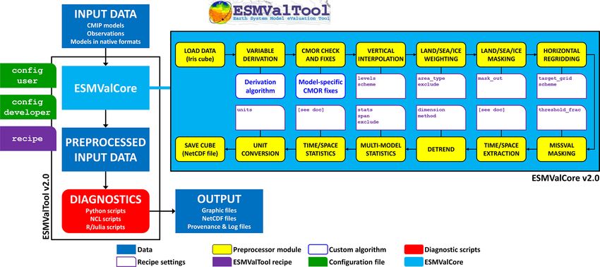
new diagnostics and analyses to the tool. A schematic repre-
files contains all the information that a diagnostic script may
sentation of ESMValTool v2.0 is given in Fig. 1.
require to be run, such as the path to the preprocessed data,
www.geosci-model-dev.net/13/1179/2020/ Geosci. Model Dev., 13, 1179–1199, 20201182 M. Righi et al.: ESMValTool v2.0 – technical overview
Figure 1. Schematic representation of ESMValTool v2.0.
the list of input datasets, the variable metadata, the diagnos- An ESMValTool v2.0 recipe consists of four sections: doc-
tic settings from the recipe, and the destination path for re- umentation, preprocessors, datasets, and diagnostics. Within
sult files and plots. The interface files are written by the ES- each of these sections, settings are given as lists or as ad-
MValCore preprocessor in the same language as the recipe ditional nested dictionaries for more complex settings. This
(YAML; see Sect. 3), which highly simplifies the coupling. allows controlling many options and features at different lev-
An exception is NCL, which does not support YAML and for els in an intuitive way. The diagnostic package contains many
which a dedicated interface file structure has been introduced example recipes that can be used as a starting point to create
based on the NCL syntax. more complex and extensive applications (see the compan-
ESMValTool v2.0 adopts modern standards for storing ion papers for more details). In the following, each of the
configuration files (YAML v1.2), data (netCDF4), and prove- four sections of the recipe is described. A few ESMValTool
nance information (W3C-PROV, using the Python package recipes are provided in the Supplement as a reference.
prov v1.5.3). Professional software development approaches
such as code review (through GibHub pull requests), auto- 3.1 Documentation section
mated testing and software quality monitoring (static code
analysis and a consistent coding style enforced through unit This section of the recipe provides a short description of its
tests) ensure that ESMValTool is reliable, well-documented, content and purpose, together with the (list of) author(s) and
and easy to maintain. These quality control practices are en- project(s) which supported its development and the corre-
forced for the ESMValCore package. For the diagnostic, code sponding reference(s). All these entries are specified using
standards are somewhat more relaxed, since compliance with tags which are defined in the references configuration file
all of these standards can be quite challenging and may in- (config-references.yml) of ESMValTool. At run time,
troduce unnecessary hurdles for scientists contributing their the recipe documentation is collected by the provenance log-
diagnostic code to ESMValTool. ger (see Sect. 5.2), which translates the tags into full text
string and adds them to the output produced by the recipe
itself.
3 New recipe format
3.2 Datasets section
To allow a flexible and comprehensive user control on the
many new features of ESMValTool v2.0, a new format for This section replaces the MODELS section used in ESMVal-
the configuration files defining datasets, preprocessing oper- Tool v1.0 namelists, and it is now called datasets to ac-
ations, and diagnostics (the so-called recipe) is introduced: count for the fact that not only models but also observations
YAML is used to improve user readability of the numerous or reanalyses can be listed here. The datasets to be processed
settings and to facilitate their passing through to the diagnos- by all diagnostics in the recipe are provided as a list of dic-
tics code, as well as the communication between ESMVal- tionaries, each containing predefined sets of key–value pairs
Core and the diagnostics. that unambiguously define the dataset itself. The required
keys depend on the project class of the dataset (e.g., CMIP3,
Geosci. Model Dev., 13, 1179–1199, 2020 www.geosci-model-dev.net/13/1179/2020/M. Righi et al.: ESMValTool v2.0 – technical overview 1183
CMIP5, CMIP6, OBS, obs4mips) and are defined in the de- 3.4 Diagnostics section
veloper configuration file (config-developer.yml) of the
tool. Typically, the user does not need to edit this file but In the diagnostics section one or more diagnostics can be
only to provide the root path to the data in the user config- defined. Each diagnostic is identified by a name and contains
uration file (config-user.yml). Based on the information one or more variables and one or more diagnostic scripts.
contained in both files, the tool reconstructs the full path of The variables and the scripts are defined as subsections of
the dataset(s) to locate the input file(s). During the ESMVal- the diagnostics section. This nested structure allows for the
Tool execution, the dataset dictionary is always combined easy definition of complex diagnostics dealing with multi-
with the variable dictionary defined in the diagnostic section ple variables and/or applying multiple diagnostics scripts to
(see Sect. 3.4) into a single dictionary, such that the key– the same set of variables. Within the variable dictionary, ad-
value pairs for the dataset and for the variable can be given ditional settings can be defined, such as the preprocessor to
in either dictionary. This has several advantages, for example be applied (as defined in the preprocessor section), the ad-
the same dataset can be defined for multiple variables from ditional variable-specific datasets which are not included in
different MIPs (such as the CMIP5 “Amon” and “Omon”), the datasets section, and other variable-specific settings used
just defining the common keys in the dataset dictionary and by the diagnostic. The same can be done for the scripts dic-
the variable-specific one (e.g., mip) in the variables dictio- tionary by providing a list of settings to customize the run-
naries. The tool collects the dataset information by combin- time behavior of a diagnostic, together with the path to the
ing the keys from the two dictionaries, depending on the vari- diagnostic script itself. This feature replaces the language-
able currently processed. This also makes the recipe more specific cfg files that were used in ESMValTool v1.0 and
compact, since common keys, such as project class or time allows the centralization of all user-configurable settings in
period, have to be defined only once and not repeated for all a single file (the recipe). Note that the diagnostic scripts sub-
datasets. As in v1.0, the datasets listed in the datasets sec- section can be left out, meaning that it is possible to only
tion are processed for all diagnostics and variables defined in apply a given preprocessor to one or more variables without
the recipes. Datasets to be used only by a specific diagnostic any further analysis, i.e., to use ESMValTool just for prepro-
or providing only a specific variable can be added as addi- cessing purposes.
tional datasets in the diagnostic or in the variable dictionary,
respectively, using exactly the same syntax. 3.5 Advanced recipe features
3.3 Preprocessor section In an ESMValTool v2.0 recipe, it is also possible to make
use of the anchor and reference capability of the YAML for-
This is a new feature of ESMValTool v2.0: in the mat in order to avoid code duplication by reusing already
preprocessors section, one or more sets of preprocessing defined recipe blocks and to keep the recipe compact. A list
operations (preprocessors) can be defined. Each preproces- of settings given in a diagnostics script dictionary can, for
sor is identified by a unique name and includes a list of op- instance, be anchored and referenced in another script dic-
erations and settings (see Sect. 4 for details). Once defined, tionary within the same recipe, while changing only some of
a preprocessor can be applied to an arbitrary number of vari- the settings in the list: a typical application is when the same
ables listed in the diagnostics section. This applies also when diagnostic is applied to multiple variables using a different
variable-specific settings are given in the preprocessor: it is set of contour levels for each plot each time while keeping
possible, for example, to set a reference dataset as a target other settings identical.
grid for the regridding operator with the reference dataset be- Another feature is the possibility of defining ancestors, i.e.,
ing different for each variable. When parsing the recipe, the tasks that have to be completed before a given diagnostic can
tool automatically replaces these settings in the preprocessor be run. This is useful for complex recipes in which a diagnos-
definition with the corresponding variable settings, depend- tic collects and plots the results obtained by other diagnos-
ing on the preprocessor-variable combination. The usage of tics. For example in recipe_perfmetrics_CMIP5.yml,
the YAML format makes all these operations quite intuitive the grading metrics for individual variables across many
for the user and easy to implement for the developer. The pre- datasets are pre-calculated and then collected by another
processor section in a recipe is optional and can be omitted script, which combines them into a portrait diagram.
if only the default preprocessing of the data is desired. The
default preprocessor will apply fixes to the data (if required),
4 Data preprocessing
perform CMOR (Climate Model Output Rewriter) compli-
ance checks, and select the data for the requested time frame A typical requirement for the analysis of output from ESMs
only. is some preprocessing of the input data by a number of oper-
ators which are quite common to many analyses and include,
for instance, temporal and spatial subsetting, vertical and
horizontal regridding, masking, and multi-model statistics.
www.geosci-model-dev.net/13/1179/2020/ Geosci. Model Dev., 13, 1179–1199, 20201184 M. Righi et al.: ESMValTool v2.0 – technical overview As mentioned in the introduction, in ESMValTool v1.0 these provide lazy evaluation (meaning that the actual data do not operations were performed in two different parts of the tool: have to be loaded into the memory before they are really at the preprocessor level (as part of the Python-based work- needed) and out-of-core processing, allowing Iris to perform flow manager controlling ESMValTool) and at the diagnos- at scale from efficient single-machine workflows through to tic level (distributed across the various diagnostic scripts and multi-core clusters and high-performance machines. One of only partly centralized in the ESMValTool language-specific the major advantages of Iris, which motivated its adoption for libraries). In ESMValTool v2.0, the code for these prepro- the revised ESMValTool preprocessor, is its ability to load cessing operations is moved from the diagnostic scripts to large datasets as cubes and to pass these objects from one the completely rewritten and revised preprocessor within the module to another and alter them as needed during the pre- ESMValCore package. processor workflow, while keeping all these stages in mem- The structure of the revised preprocessor is schematically ory without need for time-intensive I/O operations. Each of depicted in the light blue box in Fig. 1: each of the prepro- the preprocessor modules is a Python function that takes an cessor functionalities is represented by a yellow box and can Iris cube and an optional set of arguments as input and re- be controlled by a number of recipe settings, depicted by the turns a cube. The arguments controlling the operations to be purple tabs. Some operations require user-provided scripts, performed by the modules are in most cases directly spec- e.g., for variable derivation or fixes to the CMOR format, ified in the ESMValTool recipe. This makes it easy to read which are represented by the blue tabs. The figure shows the the recipe and also allows simple reuse of the ESMValTool default order in which these operations are applied to the in- preprocessor functions in other software. put data. This order has been defined in a way that minimizes In addition to Iris, NumPy (v1.17, https://numpy.org/, the loss of information through the various steps, although last access: 20 February 2020), and SciPy (v1.3.1, https: it may not always be the optimal choice in terms of per- //www.scipy.org/, last access: 20 February 2020) for generic formance (see also Sect. 4.6). For example, regridding and array and mathematical/statistical operations, the ESMVal- multi-model statistics are applied before temporal and spa- Tool preprocessor uses some specialized packages like tial averaging. This default order can be changed and cus- Python-stratify (v0.1, https://github.com/SciTools-incubator/ tomized by the user in the ESMValTool recipe, although not Python-stratify, last access: 20 February 2020) for vertical all combinations are possible: multi-model statistics, for in- interpolation, ESMPY (v7.1.0, https://www.earthsystemcog. stance, can only be calculated after regridding the data. org/projects/esmpy/, last access: 20 February 2020) for re- The ESMValTool v2.0 preprocessor is entirely written in gridding of irregular grids, and cf_units (v2.1.3, https:// Python and takes advantage of the Iris library (v2.2.1) devel- github.com/SciTools/cf-units, last access: 20 February 2020) oped by the Met Office (Met Office, 2010–2019). Iris is an for standardization and conversion of physical units. Sup- open-source, community-driven Python 3 package for ana- port for geographical maps is provided by the Cartopy li- lyzing and visualizing Earth science data, building upon the brary (v0.17.0, https://scitools.org.uk/cartopy/, last access: rich software stack available in the modern scientific Python 20 February 2020) and the Natural Earth dataset (v4.1.0, ecosystem. Iris supports reading several different popular https://www.naturalearthdata.com/, last access: 20 Febru- scientific file formats, including netCDF, into an internal ary 2020). format based on the Climate and Forecast (CF) Metadata In the following, the ESMValTool preprocessor operations Convention (http://cfconventions.org/, last access: 20 Febru- are described, together with their respective user settings. ary 2020). Iris preserves the metadata that describe the data, A detailed summary of these settings is given in Table 1. allowing users to handle their multi-dimensional data within a meaningful, domain-specific context and through a rich and 4.1 Variable derivation expressive interface. Iris represents multi-dimensional data and the associated metadata for a single phenomenon through The variable derivation module allows the calculation of vari- the abstraction of a hypercube, also known as Iris cube, i.e., ables which are not directly available in the input datasets. a multi-dimensional numerical array that stores the numer- A typical example is total column ozone (toz), which is ical values of a physical variable, coupled with a metadata usually included in observational datasets (e.g., ESACCI- object that fully describes the actual data. Iris cubes allow OZONE; Loyola et al., 2009; Lauer et al., 2017), but it is not users to perform a powerful and extensive range of cube op- part of the CMIP5 model data request. Instead the model out- erations from simple unit conversion, subsetting and extrac- put includes a three-dimensional ozone concentration field. tion, merging and concatenation to statistical aggregations In this case, an algorithm to derive total column ozone from and reductions, regridding and interpolation, and arithmetic the ozone concentrations and air pressure is included in the operations. Internally, Iris keeps pace with the modern de- preprocessor. Such algorithms can also be provided by the velopments provided by the scientific Python community, to user. A corresponding custom CMOR table with the required ensure that users continue to benefit from advances in the variable metadata (standard_name, units, long_name, etc.) Python ecosystem. In particular, Iris takes advantage of Dask must also be provided, since this information is not avail- (v2.3.0, https://dask.org/, last access: 20 February 2020) to able in the standard tables. Variable derivation is activated in Geosci. Model Dev., 13, 1179–1199, 2020 www.geosci-model-dev.net/13/1179/2020/
M. Righi et al.: ESMValTool v2.0 – technical overview                                                                                             1185

Table 1. Overview of the preprocessor functionalities and related recipe settings.

     Functionality             Key                       Possible values                  Description
     Variable derivation       derive                    true, false                      Derive the variable from basic variables using
     (Sect. 4.1)                                                                          a derivation function
                               force_derivation          true, false                      Force derivation even if the variable is available
                                                                                          in the input data
     CMOR check and fixes                                                                 Check CMOR compliance and apply dataset-
     (Sect. 4.2)                                                                          specific fixes if required

     Vertical interpolation    levels                    (List of) level(s) (Pa) or (m)   Extract or interpolate at the given level(s)
     (Sect. 4.3)                                         dataset name                     Extract or interpolate at the levels of the given
                                                                                          dataset
                                                         reference_dataset                Extract or interpolate at the levels of the reference
                                                                                          dataset
                                                         alternative_dataset              Extract or interpolate at the levels of the alterna-
                                                                                          tive dataset
                               scheme                    linear                           Interpolate using a linear scheme
                                                         nearest                          Interpolate using a nearest-neighbor scheme
                                                         linear_extrapolate               Interpolate using a linear scheme allowing for
                                                                                          extrapolation
                                                         nearest_extrapolate              Interpolate using a nearest-neighbor scheme
                                                                                          allowing for extrapolation
     Land–sea weighting        area_type                 land                             Weigh data by land fraction of the grid cell
     (Sect. 4.4)                                         sea                              Weigh data by sea fraction of the grid cell
                               exclude                   (List of) dataset name(s)        Exclude the given dataset(s) from weighting
     Land, sea, or ice mask-   mask_out                  land                             Set grid points with more than 50 % land cover-
     ing                                                                                  age to missing
     (Sect. 4.5)
                                                         sea                              Set grid points with more than 50 % sea coverage
                                                                                          to missing
                                                         ice                              Set grid points with more than 50 % ice coverage
                                                                                          to missing
                                                         glaciated                        Set grid points with more than 50 % of glaciers
                                                                                          coverage to missing
     Horizontal regridding     target_grid               NxM                              Regrid to a N ◦ × M ◦ rectangular grid
     (Sect. 4.6)                                         dataset name                     Regrid to the same grid of the given dataset
                                                         reference_dataset                Regrid to the same grid of the reference dataset
                                                         alternative_dataset              Regrid to the same grid of the alternative dataset
                               lat_offset                true, false                      Offset the grid centers of latitude by half a grid
                                                                                          cell size
                               lon_offset                true, false                      Offset the grid centers of longitude by half a grid
                                                                                          cell size
                               scheme                    linear               Regrid using linear regridding
                                                         linear_extrapolate   Regrid using linear regridding allowing for ex-
                                                                              trapolation
                                                         nearest              Regrid using nearest-neighbor regridding
                                                         area_weighted        Regrid using area-weighted regridding
                                                         unstructured_nearest Regrid using nearest-neighbor regridding for
                                                                              unstructured data
     Missing value masking     threshold_frac            [0,1]                            Apply a uniform missing value mask
     (Sect. 4.7)

www.geosci-model-dev.net/13/1179/2020/                                                         Geosci. Model Dev., 13, 1179–1199, 2020
1186 M. Righi et al.: ESMValTool v2.0 – technical overview
Table 1. Continued.
Functionality Key Possible values Description
Detrend dimension Dimension name Detrend data along a given dimension
(Sect. 4.9) method linear Subtract the linear trend of the given dimension
from the data
constant Subtract the mean along the given dimension
from the data
Multi-model statistics statistics mean Calculate multi-model mean of the input datasets
(Sect. 4.10) median Calculate multi-model median of the input
datasets
span overlap Consider only the overlapping time period
among all datasets
full Consider the maximum time period covered by
all datasets
exclude (List of) dataset name(s) Exclude the given dataset(s) from the multi-
model calculation
reference_dataset Exclude the reference dataset from the multi-
model calculation
alternative_dataset Exclude the alternative dataset from the multi-
model calculation
Temporal statistics regrid_time Re-align time axis to new time units
(Sect. 4.8 and 4.11) frequency mon, day
extract_time Extract time between start and end date
start_year Any year
start_month [1,12]
start_day [1,31]
end_year Any year
end_month [1,12]
end_day [1,31]
extract_season Extract a specific season
season DJF, MAM, JJA, SON
extract_month Extract a specific month
month [1,12]
daily_statistics Apply daily statistics
operator mean, median, std_dev,
min, max, sum
monthly_statistics Apply monthly statistics
operator mean, median, std_dev,
min, max, sum
seasonal_statistics Apply seasonal statistics
operator mean, median, std_dev,
min, max, sum
annual_statistics Apply annual statistics
operator mean, median, std_dev,
min, max, sum
Geosci. Model Dev., 13, 1179–1199, 2020 www.geosci-model-dev.net/13/1179/2020/M. Righi et al.: ESMValTool v2.0 – technical overview 1187
Table 1. Continued.
Functionality Key Possible values Description
decadal_statistics Apply decadal statistics
operator mean, median, std_dev,
min, max, sum
climate_statistics Apply climate statistics
operator mean, median, std_dev,
min, max, sum
period full, season, month, Calculate full, seasonal, monthly, or daily climatology
day
anomalies Calculate anomalies
period full, season, month, Calculate full, seasonal, monthly, or daily anomaly
day
Spatial statistics extract_region Extract a rectangular region given the limits
(Sect. 4.8 and 4.11) start_latitude [−90, 90]
start_longitude [0, 360]
end_latitude [−90, 90]
end_longitude [0, 360]
extract_named_regions Extract a predefined named region
regions A (list of) named region(s)
extract_shape Extract one or more shapes or a representative point for
these shapes
shapefile Path to shape file
method contains Select all points contained by the shape
representative Select a single representative point of the shape
crop true, false Crop (true) or mask (false) the selected shape
decomposed true, false Mask the regions in the shape files separately, adding an
extra dimension
extract_volume Extract a depth range
z_min Depth (m)
z_max Depth (m)
extract_transect Extract a transect at a given latitude or longitude
latitude [−90,90]
longitude [0,360]
extract_trajectory Extract a transect along the given trajectory
latitude_points List of latitudes
longitude_points List of longitudes
number_point No. of points to interpolate
zonal_statistics Apply statistics along the longitude axis
operator mean, median, std_dev,
min, max, sum
meridional_statistics Apply statistics along the latitude axis
operator mean, median, std_dev,
min, max, sum
area_statistics Apply statistics along the latitude and longitude axes
operator mean, median, std_dev,
min, max, sum
volume_statistics Calculate the volume-weighted average of a 3-D field
operator mean
depth_integration Calculate the volume-weighted z-dimensional sum
Unit conversion units A UDUNITS∗ string Convert units of the input data
(Sect. 4.12)
∗ https://www.unidata.ucar.edu/software/udunits/, last access: 20 February 2020
www.geosci-model-dev.net/13/1179/2020/ Geosci. Model Dev., 13, 1179–1199, 20201188 M. Righi et al.: ESMValTool v2.0 – technical overview
the variable dictionary of the recipe setting the flag derive: The interpolation is performed by the Python-stratify pack-
true. Note that, by default, the preprocessor gives priority age, which, in turn, uses a C library for optimal computa-
to existing variables in the input data before attempting to tional performance. This operation preserves units and mask-
derive them, e.g., if a derived variable is already available in ing patterns.
the observational dataset. This behavior can be changed by
forcing variable derivation, i.e., the preprocessor will derive 4.4 Land–sea fraction weighting
the variable even if it is already available in the input data,
by setting force_derivation: true. The ESMValCore Several land surface variables, for example fluxes for the car-
package currently includes derivation algorithms for 34 vari- bon cycles, are reported as mass per unit area, where the area
ables, listed in Table 2. refers to land surface area and not grid-box area. When glob-
ally or regionally integrating these variables, weighting by
4.2 CMOR check and fixes both the surface quantity and the land–sea fraction has to
be applied. The preprocessor implements such weighting, by
Similar to ESMValTool v1.0, the CMOR check module multiplying the given input field by a fraction in the range
checks for compliance of the netCDF input data with the CF 0–1, to account for the fact that not all grid points are com-
metadata convention and CMOR standards used by ESM- pletely land- or sea-covered. This preprocessor makes it pos-
ValTool. As in v1.0, it checks for the most common dataset sible to specify whether land or sea fraction weighting has
problems (e.g., coordinate names and ordering, units, miss- to be applied and also gives the possibility of excluding those
ing values) and includes a number of project-, dataset- and datasets for which no information about the land–sea fraction
variable-specific fixes to correct these known errors. In v1.0, is available.
the format checks and fixes were based on the CMOR
4.5 Land, sea, or ice masking
tables of the CMIP5 project (https://github.com/PCMDI/
cmip5-cmor-tables, last access: 20 February 2020). This has The masking module makes it possible to extract specific
now been extended and allows the use of CMOR tables from data domains, such as land-, sea-, ice-, or glacier-covered re-
different projects (like CMIP5, CMIP6, obs4mips, etc.) or gions, as specified by the mask_out setting in the recipe.
user-defined custom tables (required in the case of derived The grid points in the input data corresponding to the speci-
variables which are not part of an official data request; see fied domain are masked out by setting their value to missing,
Sect. 4.1). The CMOR tables for the supported projects are i.e., using the netCDF attribute _FillValue. The masking
distributed together with the ESMValCore package, using module uses the CMOR fx variables to extract the domains.
the most recent version available at the time of the release. These variables are usually part of the data requests of CMIP
The adoption of Iris with strict requirements of CF compli- and other projects and therefore have the advantage of being
ance for input data required the implementation of fixes for on the same grid as their corresponding models. For example,
a larger number of datasets compared to v1.0. Although from the fx variables sftlt and sftot are used to define land-
a user’s perspective this makes the reading of some datasets or sea-covered regions, respectively, on regular and irregular
more demanding, the stricter standards enforced in the new grids. In the case of these variables not being available for
version of the tool ensure their correct interpretation and re- a given dataset, as is often the case for observational datasets,
duce the probability of unintended behavior or errors. the masking module uses the Natural Earth shape files to gen-
erate a mask at the corresponding horizontal resolution. This
4.3 Level selection and vertical interpolation latter option is currently only available for regular grids.
Reducing the dimensionality of input data is a common task 4.6 Horizontal regridding
required by diagnostics. Three-dimensional fields are often
analyzed by first extracting two-dimensional data at a given Working with a common horizontal grid across a collec-
level. In the preprocessor, level selection can be performed tion of datasets is a very important aspect of multi-model
on any input data containing a vertical coordinate, like pres- diagnostics and metric computations. Although model and
sure level, altitude, or depth. One or more levels can be spec- observational datasets are provided at different native grid
ified by the levels key in the reprocessor section of the resolutions, it is often required to scale them to a common
recipe: this may be a (list of) numerical value(s), a dataset grid in order to apply diagnostic analyses, such as the root-
name whose vertical coordinate can be used as target levels mean-square error (RMSE) at each grid point, or to calculate
for the selection, or a predefined set of CMOR standard lev- multi-model statistics (see Sect. 4.10). This operation is re-
els. If the requested level(s) is (are) not available in the input quired both from a numerical point of view (common oper-
data, a vertical interpolation will be performed among the ators cannot be applied to numerical data arrays with differ-
available input levels. In this case, the interpolation scheme ent shapes) and from a statistical point of view (different grid
(linear or nearest neighbor) can be specified as a recipe set- resolutions imply different Euclidian norms; hence data from
ting (scheme), and extrapolation can be enabled or disabled. each model have different statistical weights). The regrid-
Geosci. Model Dev., 13, 1179–1199, 2020 www.geosci-model-dev.net/13/1179/2020/M. Righi et al.: ESMValTool v2.0 – technical overview 1189
ding module can perform horizontal regridding onto user- 4.7 Missing value masking
specified target grids (target_grid) with a number of in-
terpolation schemes (scheme) available. The target grid can When comparing model data to observations, the different
either be a standard regular grid with a resolution of M × N data coverage can introduce significant biases (e.g., de Mora
degrees or the grid of a given dataset (for example, the refer- et al., 2013). Coverage of observational data is often in-
ence dataset). Regridding is then performed via interpolation. complete. In this case, the calculation of even simple met-
While the target grid is often a standard regular grid, the rics like spatial averages could be biased, since a different
source grids exhibit a larger variety. Particularly challeng- number of grid boxes are used for the calculations if data
ing are grids where the native grid coordinates do not coin- are not consistently masked. The preprocessor implements
cide with standard latitudes and longitudes, often referred to a missing values masking functionality, based on an approach
as irregular grids, although varying terminology exists. As which was originally part of the “performance metrics” rou-
a consequence, the relationship between source and target tines of ESMValTool v1.0. This approach has been imple-
grid cells can be very complex. Such irregular grids are com- mented in Python as a preprocessor function, which is now
mon for ocean data, where the poles are placed over land to available to all diagnostics. The missing value masking re-
avoid the singularities in the computational domain, thereby quires the input data to be on the same horizontal and ver-
distorting the resulting grid. Irregular grids are also com- tical grid and therefore must necessarily be performed after
monly used for map projections of regional models. As long level selection and horizontal regridding. The data can, how-
as these grids exhibit a rectangular topology, data living on ever, have different temporal coverage. For each grid point,
them can still be stored in cubes and the resulting coordinates the algorithm considers all values along the time coordinate
in the latitude–longitude coordinate system can be provided (independently of its size) and the fraction of such values
in standardized form as auxiliary coordinates following the which are missing. If this fraction is above a user-specified
CF conventions. For CMIP data, this is mandatory for all ir- threshold (threshold_fraction) the grid point is left un-
regular grids. The regridding module uses this information changed; otherwise it is set to missing along the whole time
to perform regridding between such grids, allowing, for ex- coordinate. This ensures that the resulting masks are con-
ample, for the easy inclusion of ocean data in multi-model stant in time and allows masking datasets with different time
analyses. coverage. Once the procedure has been applied to all input
The regridding procedure also accounts for masked data, datasets, the resulting time-independent masks are merged to
meaning that the same algorithms are applied while preserv- create a single mask, which is then used to generate consis-
ing the shape of the masked domains. This can lead to small tent data coverage for all input datasets. In the case of multi-
numerical errors, depending on the domain under consid- ple selected vertical levels, the missing-values masks are as-
eration and its shape. The choice of the correct regridding sembled and applied to the grid independently at each level.
scheme may be critical in the case of masked data. Using This approach minimizes the loss of generality by apply-
an inappropriate option may alter the mask significantly and ing the same threshold to all datasets. The choice of the
thus introduce a large bias in the results. For example, bilin- threshold strongly depends on the datasets used and on their
ear regridding uses the nearest grid points in both horizontal missing value patterns. As a rule of thumb, the higher the
directions to interpolate new values. If one or more of these number of missing values in the input data, the lower the
points are missing, calculation is not possible and a miss- threshold, which means that the selection along the time co-
ing value is assigned to the target grid cell. This procedure ordinate must be less strict in order to preserve the original
always increases the size of the mask, which can be partic- pattern of valid values and to avoid completely masking out
ularly problematic for areas where the original mask is nar- the whole input field.
row, e.g., islands or small peninsulas in the case of land or sea
masking. A much more recommended scheme in this case is 4.8 Temporal and spatial subsetting
nearest-neighbor regridding. This option approximately pre-
serves the mask, resulting in smaller biases compared to the All basic time extraction and concatenation functionalities
original grid. Depending on the target grid, the area-weighted have been ported from v1.0 to the v2.0 preprocessor and have
scheme may also be a good choice in some cases. The most not changed significantly. Their purpose is to retrieve the in-
suitable scheme is strongly dependent on the specific prob- put data and extract the requested time range as specified by
lem and there is no one-fits-all solution. The user needs to the keys start_year and end_year for each of the dataset
be aware that regridding is not a trivial operation which may dictionaries of the ESMValTool recipe (see Sect. 3 for more
lead to systematic errors in the results. The available regrid- details). If the requested time range is spread over multiple
ding schemes are listed in Table 1. files, a common case in the CMIP5 data pool, the prepro-
cessor concatenates the data before extracting the requested
time period. An important new feature of time concatenation
is the possibility to concatenate data across different model
experiments. This is useful, for instance, to create time series
www.geosci-model-dev.net/13/1179/2020/ Geosci. Model Dev., 13, 1179–1199, 20201190 M. Righi et al.: ESMValTool v2.0 – technical overview
combining the CMIP historical experiment with a scenario mented. Furthermore, data with a dimensionality higher than
projection. This option can be set by defining the exp key 4 (time, vertical axis, two horizontal axes) are also not sup-
of the dataset dictionary in the recipe as a Python list, e.g., ported.
[historical, rcp45]. These operations are only applied
while reading the original input data. 4.11 Temporal and spatial statistics
More specific functions are applied during the prepro-
cessing phase to extract a specific subset of data from the Changing the spatial and temporal dimensions of model
full dataset. This extraction can be done along the time and observational data is a crucial part of most analyses. In
axis, in the horizontal direction or in the vertical direction. addition to the subsetting described in Sect. 4.8, a second
These functions generally reduce the dimensionality of general class of preprocessor functions applies statisti-
data. Several extraction operators are available to subset cal operators along a temporal (daily_statistics,
the data in time (extract_time, extract_season, monthly_statistics, seasonal_statistics,
extract_month) and in space (extract_region, annual_statistics, decadal_statistics,
extract_named_regions, extract_shape, climate_statistics, anomalies) or spatial
extract_volume, extract_transect, (zonal_statistics, meridional_statistics,
extract_trajectory); see again Table 1 for details. area_statistics, volume_statistics) axis. The
statistical operators allow the calculation of mean, median,
4.9 Detrend standard deviation, minimum, and maximum along the
given axis (with the exception of volume_statistics,
Detrending is a very common operation in the analysis of which only supports the mean). An additional operator,
time series. In the preprocessor, this can be applied along depth_integration, calculates the volume-weighted
any dimension in the input data, although the most usual z-dimensional sum of the input cube. Like the subsetting
case is detrending along the time axis. The method used for operators (Sect. 4.8), these also significantly reduce the
detrending can be either linear (the linear trend along the size of the input data passed to the diagnostics for further
given dimension is calculated and subtracted from the data) analysis and plotting.
or constant (the mean along the given dimension is calcu-
lated and subtracted from the data). 4.12 Unit conversion
In ESMValTool v2.0, input units always follow the CMOR
4.10 Multi-model statistics
definition, which is not always the most convenient for plot-
ting. Degree Celsius, for instance, is for some analyses more
Computing multi-model statistics is an integral part of model
convenient than the standard kelvin unit. Using the cf_units
analysis and evaluation: individual models display a vari-
Python package, the unit conversion module of the prepro-
ety of biases depending, for instance, on model configura-
cessor can convert the physical unit of the input data to a dif-
tions, initial conditions, forcings, and implementation. When
ferent one, as given by the units argument. This function-
comparing model data to observational data, these biases
ality can also be used to make sure that units are identical
are typically smaller when multi-model statistics are con-
across all datasets before applying a diagnostic.
sidered. The preprocessor has the capability of comput-
ing a number of multi-model statistical measures: using the
multi_model_statistics module enables the user to cal- 5 Additional features
culate either a multi-model mean, median, or both, which are
passed as additional dataset(s) to the diagnostics. Additional 5.1 CMORization of observational datasets
statistical operators (e.g., standard deviation) can be easily
added to the module if required. Multi-model statistics are As discussed in Sect. 4.2, ESMValTool requires the in-
computed along the time axis and, as such, can be computed put data to be in netCDF format and to comply with
across a common overlap in time or across the full length the CF metadata convention and CMOR standards. Ob-
in time of each model: this is controlled by the span argu- servational and reanalysis products in the standard CF
ment. Note that in the case of the full-length case being used, or CMOR format are available via the obs4mips (https://
the number of datasets actually used to calculate the statis- esgf-node.llnl.gov/projects/obs4mips/, last access: 20 Febru-
tics can vary along the time coordinate if the datasets cover ary 2020) and ana4mips (https://esgf.nccs.nasa.gov/projects/
different time ranges. The preprocessor function is capable ana4mips/, last access: 20 February 2020) projects, respec-
of excluding any dataset in the multi-model calculations (op- tively (see also Teixeira et al., 2014). Their use is strongly
tion exclude): a typical example is the exclusion of the ob- recommended, when possible. Other datasets not available in
servational dataset from the multi-model calculations. Model these archives can be obtained by the user from the respec-
datasets must have consistent shapes, which is needed from tive sources and reformatted to the CF/CMOR standard using
a statistical point of view since weighting is not yet imple- the CMORizers included in ESMValTool. The CMORizers
Geosci. Model Dev., 13, 1179–1199, 2020 www.geosci-model-dev.net/13/1179/2020/M. Righi et al.: ESMValTool v2.0 – technical overview 1191
Table 2. List of variables for which derivation algorithms are available in ESMValTool v2.0 and the corresponding input variables. ISCCP is
the International Satellite Cloud Climatology Project; TOA means top of the atmosphere.
Derived variable Description Realm Input variables for derivation
alb Albedo at the surface Atmosphere rsds, rsus
amoc Atlantic Meridional Overturning Circulation Ocean msftmyz
asr Absorbed shortwave radiation Atmosphere rsdt, rsut
clhmtisccp ISCCP high-level medium-thickness cloud area fraction Atmosphere clisccp
clhtkisccp ISCCP high-level thick cloud area fraction Atmosphere clisccp
cllmtisccp ISCCP low-level medium-thickness cloud area fraction Atmosphere clisccp
clltkisccp ISCCP low-level thick cloud area fraction Atmosphere clisccp
clmmtisccp ISCCP middle-level medium-thickness cloud area fraction Atmosphere clisccp
clmtkisccp ISCCP middle-level thick cloud area fraction Atmosphere clisccp
ctotal Total carbon mass in ecosystem Land cVeg, cSoil
et Evapotranspiration Atmosphere hfls
lvp Latent heat release from precipitation Atmosphere hfls, ps, evspsbl
lwcre TOA longwave cloud radiative effect Atmosphere rlut, rlutcs
lwp Liquid water path Atmosphere clwvi, cliwi
netcre TOA net cloud radiative effect Atmosphere rlut, rlutcs, rsut, rsutcs
ohc Heat content in grid cell Ocean thetao, volcello
rlns Surface net downward longwave radiation Atmosphere rlds, rlus
rlnst Net atmospheric longwave cooling Atmosphere rlds, rlus, rlut
rlnstcs Net atmospheric longwave cooling assuming clear sky Atmosphere rldscs, rlus, rlutcs
rlntcs TOA net downward longwave radiation assuming clear sky Atmosphere rlutcs
rsns Surface net downward shortwave radiation Atmosphere rsds, rsus
rsnst Heating from shortwave absorption Atmosphere rsds, rsdt, rsus, rsut
rsnstcs Heating from shortwave absorption assuming clear sky Atmosphere rsdscs, rsdt, rsuscs, rsutcs
rsnstcsnorm Heating from shortwave absorption assuming clear sky Atmosphere rsdscs, rsdt, rsuscs, rsutcs
normalized by incoming solar radiation
rsnt TOA net downward shortwave radiation Atmosphere rsdt, rsut
rsntcs TOA net downward shortwave radiation assuming clear sky Atmosphere rsdt, rsutcs
rtnt TOA net downward total radiation Atmosphere rsds, rsut, rlut
sispeed Speed of ice to account for back and forth Sea ice siu, siv
movement of the ice
sithick Sea ice thickness Sea ice sit, sic
sm Volumetric moisture in upper portion of soil column Land mrsos
swcre TOA shortwave cloud radiative effect Atmosphere rlut, rlutcs, rsut, rsutcs
toz Total ozone column Atmosphere tro3, ps
uajet Jet position expressed as latitude of maximum Atmosphere ua
meridional wind speed
vegfrac Vegetation fraction Land baresoilFrac
are dataset-specific scripts that can be run once to generate by the respective authors). An overview of the Tier 2 and
a local pool of observational datasets for usage with ESM- Tier 3 datasets for which a CMORizing script is available
ValTool, since no observational datasets are distributed with in ESMValTool v2.0 is given in Table 3. Note that observa-
the tool. Supported languages for CMORizers are Python tional datasets CMORized for ESMValTool v1.0 may not be
and NCL. These scripts also include detailed instructions on directly working with v2.0, due to the much stronger con-
where and how to download the original data and serve as straints on metadata set by the Iris library.
templates to create new CMORizers for datasets not yet in-
cluded. The current version features CMORizing scripts for 5.2 Provenance and tags
46 observational and reanalysis datasets. As in v1.0, the ob-
servational datasets are grouped in tiers, depending on their
ESMValTool v2.0 contains a large number of recipes that
availability: Tier 1 (for obs4mips and ana4mips datasets),
perform a wide range of analyses on many different scientific
Tier 2 (for other freely available datasets), and Tier 3 (for
themes (see the companion papers). Depending on the appli-
restricted datasets, i.e., datasets which require a registration
cation, sorting and tracking of the scientific output (plots and
to be downloaded or that can only be obtained upon request
netCDF files) produced by the tool can therefore be quite
www.geosci-model-dev.net/13/1179/2020/ Geosci. Model Dev., 13, 1179–1199, 2020You can also read