Machine Learning in the Social and Health Sciences - arXiv
←
→
Page content transcription
If your browser does not render page correctly, please read the page content below
Machine Learning in the Social and Health Sciences

Anja K. Leist1*, Matthias Klee1, Jung Hyun Kim1, David H. Rehkopf2, Stéphane P. A. Bordas3, Graciela Muniz-
Terrera4, Sara Wade5

Affiliations
1
 University of Luxembourg, Department of Social Sciences – Institute for Research on Socio-Economic
Inequality (IRSEI), Esch-sur-Alzette, LU
2
 Stanford University, Department of Epidemiology and Population Health, Palo Alto, CA
3
 University of Luxembourg, Department of Engineering, Esch-sur-Alzette, LU
4
 University of Edinburgh, Centre for Dementia Prevention, Edinburgh, UK
5
 University of Edinburgh, School of Mathematics, Edinburgh, UK

*Corresponding Author: Anja K. Leist, Associate Professor, University of Luxembourg, Department of Social
Sciences – Institute for Research on Socio-Economic Inequality (IRSEI), Campus Belval, 11, Porte des
Sciences, L-4366 Esch-sur-Alzette, Luxembourg. Phone: +352 46 66 44 9581, anja.leist@uni.lu

Acknowledgements
We would like to thank Dr Benedikt Wilbertz, Dr Zhalama, Thiago Quaresma Brant Chaves, as well as the
DEMON (demondementia.com) Prevention Working Group and our colleagues at IRSEI for helpful
discussions.

Funding
This work was supported by the European Research Council (grant agreement no. 803239, to AKL).

Conflict of Interest Statement
The authors declare no conflict of interest.

       Abstract
The uptake of machine learning (ML) approaches in the social and health sciences has been rather slow, and
research using ML for social and health research questions remains fragmented. This may be due to the
separate development of research in the computational/data versus social and health sciences as well as a
lack of accessible overviews and adequate training in ML techniques for non data science researchers. This
paper provides a meta-mapping of research questions in the social and health sciences to appropriate ML
approaches, by incorporating the necessary requirements to statistical analysis in these disciplines. We map
the established classification into description, prediction, and causal inference to common research goals, such
as estimating prevalence of adverse health or social outcomes, predicting the risk of an event, and identifying
risk factors or causes of adverse outcomes. This meta-mapping aims at overcoming disciplinary barriers and
starting a fluid dialogue between researchers from the social and health sciences and methodologically trained
researchers. Such mapping may also help to fully exploit the benefits of ML while considering domain-specific
aspects relevant to the social and health sciences, and hopefully contribute to the acceleration of the uptake of
ML applications to advance both basic and applied social and health sciences research.

       Significance statement
There is great interest in the social and health sciences in the application of machine learning (ML) methods,
however, a conceptual mapping of appropriate ML approaches to research questions in the social and health
sciences has been lacking. The classification presented here may help to advance the uptake of ML in social
and health sciences while also pointing to possible limitations and ways of addressing them.
                                                                                                                 1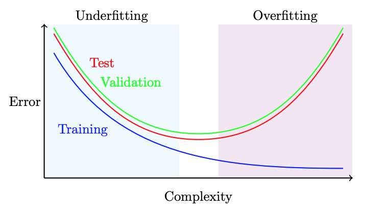
ML in the Social and Health Sciences

   Introduction
Compared to many traditional statistical methods, in particular with increasing availability of large datasets of
relevance to the social and health sciences, machine learning (ML) methods have the potential to considerably
improve aspects of empirical analysis. This includes advances in prediction, by fast processing of large
amounts of data, in detecting non-linear and higher-order relationships between exposures and confounders,
and in improving accuracy of prediction. However, uptake of ML approaches in social and health research,
spanning from sociology, psychology and economics, to social and clinical epidemiology and public health, has
been rather slow and remains fragmented to this date.

We argue that this is in part due to a lack of communication between the disciplines, the importance of
incorporating domain knowledge into statistical analysis in the social and health sciences, and a lack of
accessible overviews of ML approaches fitting the research goals in the social and health sciences. Further,
computational fields have traditionally emphasized improvements in prediction, whereas the social and health
sciences have often prioritized explanation (Yarkoni & Westfall, 2017) and the importance of domain
knowledge. There is a need to establish a fluid dialogue between researchers from the social and health
sciences and methodologically trained researchers to avoid "rediscovering the wheel". ML researchers may
overlook features of data that have been previously found to be highly relevant in the social and health
sciences (e.g., oversimplification of recoding of some variables when integrating datasets). In contrast,
researchers in the social and health sciences may not be aware of the complex mathematics and statistics
behind the algorithms and the fast progressing developments of improving ML methods, and how the
mathematical commonality between different domain problems can be leveraged to improve the efficiency of
data-driven research (Ley & Bordas, 2018).

The aim of this paper is to provide a high-level, non-technical toolbox of ML approaches through the systematic
mapping of research goals in the social and health sciences to appropriate ML methods. These can be built on
top of each other or combined with more traditional methods. We will further point researchers to solutions to
common problems in ML modelling. As we have strong interests in the social and behavioural determinants of
health and disease, many applications mentioned here focus on relevant research and possible ML
approaches in the fields of psychology, social epidemiology, and prevention research.

This conceptual overview should be seen as complementary to several introduction papers to machine
learning in the fields of epidemiology and health research (Wiemken & Kelley, 2020), psychology (Yarkoni &
Westfall 2017), and helpful glossaries (Bi et al., 2019). For general introductions to statistical learning,
interested readers are referred to several excellent textbooks on these approaches (Efron & Hastie, 2016; J.
Friedman et al., 2001; Hardt & Recht, 2021; James et al., 2013). The changed research infrastructure and
computational requirements when using machine learning and issues of privacy have been discussed
elsewhere (Fuller et al., 2017; Mooney & Pejaver, 2018) and will not be covered here.

While some of the ML approaches presented here require more domain knowledge than others, for example
ML for causal inference, we argue that in all research questions in the social and health sciences substantial
domain knowledge is necessary to meaningfully contribute to the field, and that this is a prerequisite to
interpretability (Murdoch et al., 2019). Agnostic data exploration alone will in most cases provide fewer insights.
Generally, from our own experience, we recommend collaborations across disciplines by inviting data science
and machine learning experts to do research in the social and health sciences, and hope the mapping
presented here will facilitate mutual understanding of the different disciplines.

We present here, adapted to the social and health sciences, a classification of machine learning tasks for
description, prediction, and causal inference (Hernan, Hsu & Healy 2018), even if not all research questions
allow such strict distinctions. We will illustrate this mapping with studies from the social and health sciences.
The methods summarized as ML in this overview represent different traditions of data analysis, e.g. inferential
statistics, statistical learning, and computational sciences, their common denominator is the ability to process
large amounts of data while making model-building and model selection decisions more driven by the structure
                                                                                                                  2
ML in the Social and Health Sciences
of the data (data-driven) than traditional inferential statistics. First, we provide a set of basic terms and the ML
workflow and general points on interpretability, fairness, and generalizability, before describing the ML tasks in
more detail.
Background to ML approaches
ML approaches will usually involve the ‘training’ (estimation) of a model in a so-called training data set and, in
a second step, the ‘testing’ of the model regarding its performance (e.g., accuracy of classification) in a
separate test data set. ML approaches can be categorized into unsupervised learning, supervised learning,
and reinforcement learning:
● Unsupervised learning is an umbrella term for algorithms that learn patterns from unlabelled data, that
is, variables that are not tagged by a human. For instance, unsupervised learning will group data
instances based on similarity.
● Supervised learning comprises algorithms that learn a function which maps an input to an output, by
using labelled data, that is, the values of the categories of the outcome variable are assigned
meaningful tags or labels. Input would in the social and health sciences be termed predictors,
independent variables or exposures, and covariates; output would be termed outcomes or dependent
variables. Supervised learning requires labelled training data and can be validated in a labelled test
data set. We will present neural networks (often called artificial neural networks, ANNs) as an example
of a predictive algorithm (Box 1), and Bayesian Additive Regression Trees (BART) as an example of
ML for causal inference (Box 2). Transfer learning will transfer learnt features from one situation to
another (congruent) situation, thereby identifying patterns and behaviours common to a variety of
situations. While often employed with labelled data and thus mentioned as approach specific to
supervised ML, transfer learning approaches have also been developed for image recognition and
other applications not covered in this review.
● Reinforcement learning is concerned with an intelligent agent taking decisions to an environment and
improves based on the notion of cumulative reward, i.e. the agent will vary and optimize the input
based on the feedback from the environment. Reinforcement learning can be applied in contexts where
data generation, that is, manipulation of a treatment variable (so called A/B testing) under control of
other features (covariates) is possible.
Most ML approaches presented here will require large(r) datasets than traditional modelling for the models to
outperform traditional modelling in new data sets. Some aspects of the data should be available at a larger
quantity, such as time points, variables, or individuals. Rule of thumb would be to have several ten thousand
data points available, but some applications have used very small datasets for exploratory analyses (Wiemken
& Kelley 2020). Similar to non-ML analyses, careful processing of data (e.g., during the harmonization
process), a deep understanding of where the data are coming from, what they can tell us (and what they
cannot), is vital. The ML workflow has been described in several introductory papers, see Wiemken & Kelley
(2020) for a recent overview.
In this paper, we will not cover ML algorithms that have been developed for more automatic processing of big
data, such as speech recognition and sentiment analysis. These algorithms have been specifically developed
to increase speed and efficiency of analysis of speech, text or images. Use of ML in these fields indeed provide
numerous advantages over traditional procedures in qualitative social research such as higher efficiency and
accuracy in retrieving summary features. Other use cases of ML concern the anonymisation of electronic
health records to ensure GDPR regulations prior to analysing sensitive data or the preparation of
infrastructures to analyse large datasets most efficiently (e.g. reinforcement learning to optimize batching of
data to be analysed). Our review focuses on research questions that involve datasets with human participants
as research units and the analysis of clinically assessed or self-reported variables.
In the following, we present a few additional aspects of particular relevance to the social and health sciences.
In the data preparation process, researchers need to prepare exposure and outcome variables (so-called
3ML in the Social and Health Sciences
feature selection and engineering) in a way the algorithm understands: Feature selection, that is, reducing the
number of variables to be processed by the model by applying the minimal redundancy maximal relevance
criterion, may be helpful in large datasets such as the PISA survey or aging surveys from the family of Health
and Retirement Studies. Conceptually interesting features, for example cumulative risk (multiplicative effect of
two predictors) or changes between measurements (e.g. weight loss over time) are not well detectable by
including the single variables. We suggest to explore if the reduction of complexity in the set of (related)
independent variables makes sense, e.g. factor analysis or cluster analysis, and/or selection of variables
based on theory. If the dataset is large enough, a rule of thumb here is the availability of several 10,000
relevant units (e.g. respondents to a survey), this enables the use of neural networks, which are well known to
use feature engineering in the generation of the models. While it is necessary to make the continuous variables
equivalent in variance, we would recommend using manual feature engineering only to an extent to which
researchers in the social and health sciences can still ensure some interpretability for real-world applications.
On the other hand, traditional modelling is highly depending on researcher decisions (e.g., modelling a
quadratic instead of a linear relationship, modelling interaction effects manually). Here, algorithm-based
decisions regarding feature engineering for example in neural networks can provide more robust and accurate
findings. Approaches like BART (described in more detail below) will handle the simultaneous inclusion of
continuous, dichotomous and categorical predictors. In contrast, other approaches such as regression trees
will overvalue continuous predictors simply due to the availability of a larger number of possible splitting points,
however rules for splitting decisions for categorical variables exist in some algorithms, but are handled
differently across software packages.
In feature engineering, researchers should always be conscious of the curse of dimensionality, which
describes the tendency of the test error to increase as the dimensionality of the problem increases, unless
additional features are truly associated with the response (i.e., not just adding noise). More features, that is,
variables in the model, increase the dimensionality of the problem, exacerbating the risk of overfitting. Thus,
advances in data acquisition that allow for the collection of thousands or even millions of features are a double-
edged sword; improved prediction can result if the features are truly relevant and the sample is population-
representative, but they will lead to more biased results if not. Moreover, even if they are relevant, the
reduction in bias may be outweighed by increased variance incurred by their fit (James et al., 2013). Evaluating
the quality and performance of the model, ML models offer less straightforward solutions compared to more
traditional modelling in the social and health sciences. To overcome this, we have compiled a table with an
overview of model performance indicators for each of the ML approaches (table 2). Particularly ML for
regression and classification can also be compared against traditional methods to see the value gained.
Researchers also need to be aware of the trade-off between increasing predictive accuracy and overfitting,
ideally through proper cross-validation procedure. Most researchers will be familiar with the ML modelling
process which comprises splitting the data into a training and a test set, possibly also a third partition which is
held-out of the train-test iterations for later model evaluation. External cross validation further allows testing the
generalization error of resulting models. In newer packages such as the SuperLearner (a.k.a. stacking) that
wraps a number of different algorithms to increase model performance, solutions are in-built already. It is
preferred to additionally validate models in new datasets (neither used for training nor test). We illustrate this
trade-off between predictive accuracy and overfitting in Figure 1, which highlights the typical interrelation of
training, validation, and test errors. The training error typically decreases with model complexity, while the
validation and test curves have a U-shape. Underfitting refers to the case when a more complex model
improves the test error, and overfitting occurs when a less complex model yields a lower test error. We almost
always expect the training curve to lie below the test curve, as most methods aim to minimize the training error.
Importantly, the test data is held-out in model training in order to provide a realistic measure of performance,
thus validation methods, which split the training dataset, are employed to select complexity and tuning
parameters. The validation curve typically lies above the test curve, since it is trained on a smaller training set,
and can also be highly variable due to the random data splits. However, the goal of validation is to identify the
correct level of flexibility, i.e. the minimum point of the test error. Cross-validation is typically used to help
reduce the variability in the validation curve. However, it is appropriate under the assumption of independent
4ML in the Social and Health Sciences
and identically distributed data; for some data, such as time series or longitudinal data, this is not appropriate
and splits must account for the structure in the data. When the validation curve is relatively flat, the simpler
model is preferred.
AutoML approaches such as the H2O.ai interface aim to facilitate the ML workflow for non data science
researchers (H2O.ai, 2021; LeDell & Poirier, 2020). AutoML by default trains and cross-validates generalized
linear models, gradient-boosting machines, random forests, deep neural networks and combines via
SuperLearning/stacking to improve model fit. While easy-to-use interfaces are attractive to non data sciences
researchers and can be helpful in many cases, we argue that, similar to research with traditional inferential
statistics, an understanding of the applied methods in greater detail is still necessary for substantial research
contributions.
Figure 1. Typical relationship between model error and complexity.
General points
In the following, we will refer to relevant concepts when applying ML in the social and health sciences,
specifically, interpretability, fairness, and generalizability.
Interpretability / explainability and visualization
Interpretable ML means to extract relevant knowledge from ML models, i.e. able to feed into the domain
knowledge of a discipline, characterized by predictive accuracy, descriptive accuracy and relevancy, with
relevancy judged relative to a human audience (Murdoch et al., 2019). Interpretability is important in high-stake
decisions, such as clinical decision making. Here new developments exist to increase acceptance, e.g. the
symbolic metamodeling framework for interpreting predictions by converting “black-box” models into “white-
box” functions that are understandable to humans (Alaa & van der Schaar, 2019). Others have however
suggested that the use of separate, explainable, models could be problematic in applications as there is still
limited transparency for the users of the ML models (Rudin, 2019).
Interpretability is in practice often linked with the possibility to visualize the estimated or discovered
relationships among variables. Summary packages intended to give a user-friendly set of possibilities to
increase (post-hoc) interpretability have been developed, e.g. iml (Molnar et al., 2018). To increase
interpretability, bi-variate and higher-order data associations with possible non-linear patterns or missing data
that are not at random, as well predictions can be visualized e.g. with partial dependence plots (Greenwell,
5ML in the Social and Health Sciences
2017), SHAP plots (Lundberg et al., 2018; Mangalathu et al., 2020), or Individual conditional expectation (ICE)
plots, a newer and less well-known adaptation of partial dependence plots (P. Hall et al., 2017).
Fairness
A relevant notion in the health and social sciences is the idea of the ML algorithm to decide “fairly”, i.e. will not
discriminate against certain social or minority groups. Here, particularly in the application of ML in high-stake
decision making such as predicting recidivism, predictive model accuracy needs to be balanced against the
model treating all social groups equally, i.e. the ML model resulting in all social groups having equal probability
of receiving a desirable outcome. We refer to other literature for considerations regarding fairness in ML at
large (Barocas et al., 2017) and ethics in ML in the human and social sciences (Lo Piano, 2020). Importantly,
health equity efforts can be undermined by structural discrimination/racism possibly implemented in ML
diagnosis or decision-making (Rajkomar et al., 2018; Robinson et al., 2020). Outside the scope of our review, it
is critical to realize that fairness is not just important in application of algorithms, but in the full arc of the
research process (Chen et al., 2020).
Generalizability or external validity
The importance of generalizability of external validity is not limited to ML approaches: Across research designs
as well as across stages of data collection, we need to consider biases that could harm generalizability, as it is
desired that findings have validity beyond the dataset in which they were discovered. In the context of ML, it is
important to mention the risk of overfitting, i.e. to improve model accuracy within the dataset by risking model
performance in a new dataset. An example of how differences in recruitment in cohort studies can result in
differential performance of ML algorithms is (Birkenbihl et al., 2020). And, similar to more traditional analyses,
triangulation of methods is recommended (Matthay et al., 2020). While in the past it has been stated that a lot
of ‘black art’ necessary to successfully implement ML in research (Domingos, 2012), we stress the importance
of documenting all decisions in the statistical analysis to the details (e.g. specifying seed of random number) to
ensure scientific findings are replicable.
We now move to the classification of ML approaches for description, prediction, and causal inference (some of
which admittedly have their roots in standard statistical methods), and start with ML approaches for
description.
ML for Description
A descriptive research question aims to “provide a quantitative summary of certain features of the world”
(Hernán et al., 2019). Description is the basis of all applied research, as we need description to quantify the
phenomenon under study, e.g. assess prevalence or distributions of variables between (social) groups,
countries or geographical entities, or over time (between cohorts). This can be done through several algorithms
(Table 1). Among these, researchers in the social and health sciences are aware of factor analysis of one
(cross-sectional) measurement of several variables. Dimensionality reduction can reduce complexity of
datasets for more efficient subsequent analysis (van der Maaten et al., 2009). Domain knowledge is necessary
to pre-select variables for factor analysis that are interpretable and meaningful, as cluster (and factor) analysis
cannot conceptually distinguish variables, for example, if some data are coming from humans or from other
data. Factor analysis will provide factors and factor loading for the included variables. Factors are often used
as new variables with densified information in subsequent analyses. Readers should note that algorithms
based on Bayesian modelling are available for factor analysis and other methods presented here but will not
be covered in detail. We suggest to not mix individual-level variables with higher-order variables e.g. related to
environment or neighbourhood in a factor analysis to ensure interpretability of the factors in subsequent
analyses. Another helpful approach may be cluster analysis to group data based on similarity. Unlike in factor
analyses, cluster analysis can help to process measurements of individual-level and contextual-level variables
simultaneously, for example, individual-level BMI and contextual-level air pollution to investigate different risk
6ML in the Social and Health Sciences
groups or profiles (e.g. with high BMI and high air pollution) for dementia. Finally, bi-clustering may be helpful if
samples and variables need simultaneous grouping.
Screen and identify individuals at risk or higher-level patterns
Individuals can be screened for single risk factors, through automated processing of data, for example, people
at elevated risk for adverse health outcomes can be identified through processing of Electronic Health
Records. This research goal could be solved with algorithms for anomaly detection. Conducting clustering or
factor analysis, a group of variables can be processed simultaneously, by analysing patterns across
individuals. To identify ageing-related morbidity pathways, electronic health records that contained information
on 278 high-burden diseases were analysed with different clustering algorithms to group diseases according to
their patterns of age at onset of disease (Kuan et al., 2021). To add, the complex information derived from ML
was visualized with traditional plotting, for example, distributions of onset of disease curves per disease cluster
(Kuan et al., 2021).
Longitudinal analyses of trajectories of time-varying variables can be helpful to better understand the trajectory
of previously identified risk factors with long-term observational data, preferably with minimum 5 follow-up
measurements. This can be interesting in diseases where long-term risk prediction is relevant, or where long
prodromal phases need to distinguish if factors are indeed risk factors or early symptoms. Depressive
trajectories were identified via k-means clustering of the number of depressive symptoms at each
measurement occasion over a long follow-up, to distinguish early-onset from late-onset depression (Demnitz et
al., 2020). Analyses like this can help elucidate changing risk factor importance over the life course, for
example in the field of dementia (Peters et al., 2020)
Death as a competing risk needs to be accounted for in investigations on aging-associated diseases, e.g. with
random survival forests, which also allow modelling of time-varying risk factors (Weiss et al., 2020). If a focus
is on the short-term consequences of time-varying treatment, i.e. if causal conclusions are intended, it may be
better to use established methods in the potential-outcomes framework such as marginal structural models or
the g-formula (Robins et al., 2000; Hernán & Robins 2021).
Risk profiles
To identify risk profiles, i.e. groups of individuals characterized by certain values on a set of variables, ML for
discovery can be used to describe and reduce complexity, based on previous literature that had identified risk
or protective factors. Using severity scores common in the ICU setting, patient health state trajectories were
categorized with a number of dimensionality reduction (and predictive) techniques in time-series data, among
others DBSCAN (Galozy, 2018). These health state trajectories were correlated with medication and
treatments, with commendable visualizations of the resulting patterns (Galozy, 2018).
While most descriptive research problems in the social and health sciences will require unsupervised ML, there
is no one-to-one correspondence of descriptive problems to unsupervised ML. In the following, we will present
descriptive research questions that need supervised ML approaches typically used for prediction.
Diagnosis
A descriptive research goal is to identify prevalence of a health outcome, which can be reasonably inferred
also in absence of clinical assessment. This descriptive goal of diagnosis can be accomplished with supervised
ML or a semi-supervised setting if a mix of labelled and unlabelled data is analysed. With data from electronic
health records (EHR), algorithms can, in the absence of human clinical assessment, identify the existence of
characteristics (or joint presence of conditions) that increase likelihood of a presence of disease, for example
through neural networks. Other data, such as sensor data, language data etc. can be used to detect conditions
or disease. Movement of sign language users was analysed to detect likely dementia with convolutional neural
networks (Liang et al., 2020).
7ML in the Social and Health Sciences
In the absence of a diagnosis based on clinical assessments, classifying individuals with a probable diagnosis
through ML may be interesting to estimate population-level disease prevalence and associated healthcare
costs. Identifying individuals with probable diagnosis is unobtrusive and may be more cost-effective than the
clinical assessment of these individuals. Combining PCA and cluster analysis, participants with high likelihood
of dementia were identified in U.S. and European datasets (de Langavant et al., 2018) and with datasets from
across the world (de Langavant et al., 2020). With cultural and education fair battery of cognitive tests, the
10/66 diagnosis of dementia can be done with cognitive tests alone to improve prevalence of dementia
estimations in the absence of possibilities for clinical assessment, with application of machine learning to data
from South India (Bhagyashree et al., 2018).
Supplementing classifications of probable diagnosis with diagnosed individuals may address underreporting
and underdiagnosis of conditions such as dementia. These individual-level probable diagnoses can be used to
investigate risk and protective factors of these conditions. Survey participants were identified as having
probable dementia with a mix of traditional and ML based (descriptive and predictive) algorithms, and with the
aim to provide dementia classification algorithms with similar sensitivity/specificity across racial/ethnic groups
(Gianattasio et al., 2020). ML in this study proved more complex to implement and was considered more
sensitive to cohort and study procedural differences than traditional modelling; additionally, use of ML, in this
case LASSO and the SuperLearner, did not lead to increases in model performance compared to different
expert models (Gianattasio et al., 2020). Samples of less than 2,000 participants may thus be less
recommended for the use of ML approaches.
Table 1. Overview and non-technical description of ML methods for description most relevant in the
social and health sciences
ML for Description
Clustering:
Clustering groups data based on similarity. Examples are
● k-means: clusters data points according to a distance metric in an n(variables)-dimensional
space
● Hierarchical agglomerative clustering: starting from each object forming a separate cluster,
clusters are consecutively merged moving up the hierarchy
● Model-based clustering: the most widely-used example is the Gaussian mixture model
(GMM), which generalizes k-means by allowing elliptically-shaped cluster.
● Density-based spatial clustering of applications with noise (DBSCAN) (Ester et al., 1996;
Schubert et al., 2017) groups data points in spatial proximity while marking data points in
low-density regions as outliers.
● Mixtures of experts (learners): This approach divides the input space in homogeneous
regions, and a different expert is responsible for each region. This allows for different
clusters, e.g. of patients, with different (non)linear relationships between y and x (Jordan &
Jacobs, 1994; Masoudnia & Ebrahimpour, 2014).
Dimensionality reduction
● Principal component analysis (PCA): Known to researchers in the social and health
sciences, this method provides a low-dimensional approximation/encoding of the data by
linear (orthogonal) projection (i.e. low-dimensional features are linear combinations of the
original features)
● Probabilistic principal component analysis (PPCA) is a probabilistic model formulation of
PCA for higher-dimensional data such as found in metabolomics. The PPCA will provide
the PCA solution in limit of zero noise (Tipping & Bishop, 1999)
● Factor Analysis: Also known to researchers in the social and health sciences in the
analysis of, for instance, questionnaire-based data, factor analysis can be seen as a
8ML in the Social and Health Sciences
generalization of PPCA that allows dimension-specific noise. This method explains the
correlation across dimensions through a small number of latent factors.
● Independent Component Analysis: generalization of FA that allows the distribution of the
latent factors to be any non-Gaussian distribution.
● Nonlinear dimension reduction: includes kernel PCA, Gaussian process latent variable
model (GPLVM), t-SNE (Van der Maaten et al. (2009).
● Generative Adversarial Networks (GANs): The task of grouping data points based on
similarity is split into a two-part problem of, first, generation of new data that should be
similar to the real data, and the task of, similar to supervised learning, classifying the data
as either real or new (fake). The task stops once the algorithm is no longer able to
discriminate real from new data (Goodfellow et al., 2014).
● Variational Autoencoders (VAEs) employ neural networks for dimensionality reduction,
both for encoding and decoding (mapping the data to the low-dimensional latent space and
v.v.). VAEs use a probabilistic formulation and variational inference to learn the distribution
of the latent variables, which avoids overfitting and imposes desirable properties on the
latent space (Kingma & Welling, 2013)
Anomaly detection
This is the process of identifying data points that deviate from normal “behaviour”, that is, is
identified as dissimilar in the context of the overall data points. Anomalous data may indicate an
incident, deviant behaviour (e.g. fraud in data of bank transfer, changes in household composition
of a consumer in consumption data).
Biclustering
As a newer development, one may also be interested in the simultaneous grouping samples
(individuals) and features (variables) based on similarity. The so-called biclustering methods
simultaneously cluster samples and features (for a recent review: Padilha & Campello 2017).
Biclustering is used in bioinformatics, e.g. to cluster patients based on expression profiles on a
subset of genes (Moran et al. 2020).
ML for Prediction
The ML task of prediction will need mapping some features (input) to other, known, features (output) as
accurately as possible (Hernán et al., 2019). Again, known outcomes like a health outcome are called labelled
data; to investigate predictive research questions, we thus employ supervised learning: As explained above,
supervised learning is the ML task of learning a function from labelled data to map an “input” (predictors,
independent variables) to an “output” (outcome). Numerical (continuous) outcomes will require regression
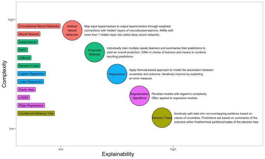
techniques, while dichotomous or categorical outcomes will require classification techniques. Figure 2 presents
an overview of ML methods that are, based on theoretical considerations, ranked to explain the trade-off
between explainability versus complexity of these methods.
9Note. Ordering and selection of ML methods based on theoretical considerations.
Figure 2. ML methods for prediction most relevant in the social and health sciences with non-technical description ranked by
interpretability/explainability versus complexity.
10As a few popular and/or well-performing ML methods, typical ML methods to solve predictive problems are
penalized regression methods, ensemble learning, gradient boosting, decision trees, and neural networks (see
Figure 2). Neural networks are described in more detail in Box 1. Shrinkage or penalized regression methods
(e.g. LASSO, ridge regression, elastic nets) are also used in “traditional” inferential statistics. Penalized
regression performs better than the standard linear model in large multivariate data sets where more variables
than individuals are available. Penalized regression will add a constraint in the equation to penalize linear
regression models with too many variables in the model, also called “shrinkage” or “regularization”. This will
shrink the coefficient values towards zero, so less contributive variables will have coefficients close to zero or
equal zero (Hastie et al., 2009). Ensemble learning improves predictive accuracy by using multiple descriptive
and predictive ML algorithms. An example family of algorithms is the SuperLearner that has been applied in
epidemiological research questions (Naimi & Balzer, 2018). The SuperLearner uses cross-validation to
estimate the performance of several descriptive and predictive ML models, or in the same model with different
settings, and works asymptotically as accurately as the best prediction algorithm used in the model fitting
process. Due to their interpretability, decision tree algorithms and ensemble methods such as Random Forests
(Svetnik et al., 2003), have been employed in numerous studies in the social and health sciences.
Commended for its high predictive accuracy and robust applicability to many predictive problems, we point
readers to stochastic gradient boosting (J. H. Friedman, 2002), which has been implemented in ready-to-use
packages in python and R for the family of Gradient Boosting algorithms, for example in the recommended
xgboost package. Through boosting, the typical problem of collinearity of input variables (predictors) does not
occur, that means that differently engineered (pre-processed) variables can be entered simultaneously to see
which characteristics are most predictive. Researchers need to be aware that the algorithm does an exhaustive
search over all variables for splitting-points, and some variables may be more informative to divide the sample
than others. The algorithm is thus biased towards choosing numerical (continuous), multi-category variables or
variables with missing data over dichotomous variables; methods towards unbiased variable selection are
available (Hothorn et al., 2012). Further, variables will be picked as splitting points that best explain the
dependent variable, which is not necessarily the most meaningful variable from a theoretical perspective
relevant in the social and health sciences.
Box 1: Detailed description: Artificial neural networks
A more complex way of solving prediction problems by mapping some features (predictors) to other features
(outcome) can be done with neural networks, which learn interrelationships between variables, with a
defined “input” (predictors) and “result” (outcome). Neural networks are motivated by the computation in the
brain that enables successful recognition and classification of complicated tasks (Fine 1996). Neural
networks are identical to the traditional logistic regressions with no hidden layer if logistic activation function
is implemented, which is the most common case (Dreiseitl and Ohno-Machado 2002). Both neural networks
and logistic regression have a functional form, and the parameter vector is determined by maximum-
likelihood estimation. However, neural networks allow us to relax the linearity of input variables and log odds
assumption. Consequently, it is a better option if the data is not classified linearly. This flexibility comes with
a cost of difficulty in interpretation of the parameters; the resulting model is evaluated through model
performance measures such as sensitivity, specificity, accuracy, and the area under the ROC curve (see
Table 2). Neural networks build at least one hidden layer between the input and output, and the benefits of
neural networks to increase model performance actually come from the algorithms’ capacity to develop
several hidden layers. The training process of neural networks mainly consists of two steps. Firstly, Feed
Forward takes the inputs or previously hidden layer and combines them with weights. Secondly, Backward
Propagation takes the output layer or its previous hidden layers to adjust based on the error between the
actual and the predicted values. By iteration of this feedforward and backward propagation, neural networks
train to adapt the transformation and regression parameters. If no careful process of testing and cross-
validation after training is implemented, neural networks are susceptible to overfitting. Regularisation can
solve this problem through cross-validation or bootstrapping (Harrell 2001). Another way is to utilize the
Bayesian framework. Rather than giving a point estimation, it calculates the distribution of parameters to
avoid overfitting problems (Neal, 1996). Moreover, while neural networks tend to be overconfident even
when predictions are incorrect and are vulnerable to adversarial attacks (Szegedy et al., 2013), Bayesian
neural networks, which produce an ensemble of neural networks, are robust and accurate (Carbone et al.,
2020). This may be particularly relevant to increase trust and social acceptance in social and health
11ML in the Social and Health Sciences
sciences also in the light of the trade-off in interpretability due to the complexity of the algorithms and
resulting models.
Prediction problems are highly relevant in social and health sciences: We may want to predict a certain output,
that is, health or social outcome either as accurately or as parsimoniously as possible. Research goals may be
to explain maximum variance in the outcome or find a minimal or optimal predictor set. We may want to
evaluate how well a certain input, for example, a candidate risk factor, is able to predict an outcome. Prognosis
in its simplest form is a prediction problem. There may be defined end points, and we wish to estimate the
probability of reaching one of the endpoints. With a perspective of ML as letting the computer/the algorithm
define the model instead of the human, ML can test the relative importance of one or more predictors, by
considering a large set of covariates, and provide absolute values of importance or rank-order information.
Again, the curse of dimensionality mentioned above applies. For in-depth explanations, we refer to prediction
textbooks (Kuhn & Johnson, 2013).
A typical problem in the health and social sciences is the prediction of rare outcomes, such as disease, crime,
learning difficulties, divorce, etc. where only a very small percentage of the observed population will show the
outcome of interest. For example, the rate of offenders is very small compared to the total population;
dementia is prevalent in less than 10% of the population aged 60 and older; up to one third of married people
will file for divorce. Using ML to predict rare outcomes (and rare may be defined as anything less frequent than
50% of the cases), classification algorithms will usually simply develop a model which will only predict the non-
occurrences of the outcome, since the algorithm will detect that a guess of “0” will be correct in most cases.
Researchers may solve this problem by redefining the outcome, for example, as regression instead of
classification problem. Changing the distribution of the outcome in the sample by oversampling of the group
with the rare outcome through, for example, synthetic minority oversampling technique, SMOTE (Chawla et al.,
2002), is well established. Equally, undersampling of the group without the outcome is possible. Simulated
datasets and ‘virtual cohorts’ may be useful in some cases. We discuss below transforming a rare outcome in
a more frequent one by redefining the research question.
Estimate and project prevalence of adverse social or health outcomes
Estimating disease prevalence is the basis for quantifying health burden, the need for interventions, and health
and social care planning. Estimation of the rate, incidence, or prevalence of a phenomenon under study, for
example, a health outcome such as diabetes in a certain population can be considered descriptive; the
projection of estimates would rather be predictive. An example, incorporating the social determinants of health
perspective, is to take prevalence estimations of non-communicable diseases by age, sex, and race/ethnicity
(can be done with individual-level data or aggregate data), and estimate their prevalence for unknown areas
through ML. Presence of six non-communicable diseases (NCD) was estimated through LASSO to predict
population-level prevalence of NCD with a minimal demographic dataset for 50 U.S. states (Luo et al., 2015).
Similarly, health outcomes have also been predicted on the more fine-grained neighbourhood level (Feng &
Jiao, 2021).
Predict adverse health or social outcomes
We first discuss research with the main interest in the “output”, that is, research with the aim to predict a health
or social outcome as accurately as possible. This is done by adding more information (variables) to the model,
or by accounting for higher-order interactions or non-linear relationships. Typical research questions have been
to test improved predictive accuracy of ML compared to traditional modelling, e.g. regarding the social
determinants of health (Seligman et al., 2018), the prediction of dementia (Aschwanden et al., 2020; Weiss et
al., 2020), or prediction of student drop-out (Kemper et al., 2020), with ML approaches typically not
dramatically outperforming traditional regression-based modeling. A good illustration of this research goal is a
retrospective prediction of veteran suicides. Bayesian Additive Regression Trees (BART) were the best ML
algorithm of several tested in a dataset of veteran suicides matched with a 1% random matched sample of
veterans alive at the time (Kessler et al., 2017). Other research has employed the SuperLearner for mortality
risk prediction (Rose, 2013), or penalized linear regressions to predict healthcare costs with penalized linear
12ML in the Social and Health Sciences
regressions (Kan et al., 2019). A systematic review on clinical risk prediction with machine learning found little
benefits of ML methods over regressions, and criticized a number of shortcomings in the literature up to that
date, particularly the lack of calibration, i.e. testing the reliability of predictions (Christodoulou et al., 2019).
Researchers may be aware that the more distal the predictors, the more difficult it will be to arrive at robust,
accurate predictions. As an example, a study used characteristics of correctional facilities and aggregate
inmate characteristics to predict prison violence, assessed by number of inmate-on-inmate assaults with the
SuperLearner but failed to arrive at high levels of accuracy (Baćak & Kennedy, 2019).
Interest in the “output”, that is, the health or social outcome, may also come with the aim of finding a minimal or
optimal (most parsimonious) predictor set. Coming back to the earlier mentioned example to predict
population-level prevalence of non-communicable diseases, these diseases were estimated with a minimal
socio-demographic predictor set (Luo et al., 2015). In dementia risk prediction, for which until recently no
robust algorithms were available (Licher et al., 2018), an optimal model predicting dementia over 10 years has
been recently developed with LASSO (Licher et al., 2019). Preliminary research has developed a parsimonious
model to predict differential diagnosis of dementia (Guest et al., 2020). An optimal predictor set was sought in
one study to explain variance in firearm violence, combining LASSO and random forest algorithms (Austrom et
al., 2018).
A rare outcome may be more frequent in pre-selected samples, for example, dementia research has partly
focused on improving prediction of conversion from Mild Cognitive Impairment (MCI) to dementia. At-risk
samples of people with MCI may be used to train a model that discriminates converters from non-converters
based on questionnaire-, biomarker- or imaging-based variables. Among numerous examples, some studies
tested the role of cognitive reserve to predict conversion to dementia with different ML algorithms (Facal et al.,
2019), and tested their model developed with a support vector machine algorithm in new subjects (Grassi et
al., 2019). While dementia risk prediction models improve substantially particularly after adding genetic and
imaging information to the models, there is no significant progress in the ability to predict decline of cognitive
performance tests in at-risk samples (Marinescu et al., 2020).
In clinical practice, the relevant “output” may not be an adverse health outcome, but the necessity to intervene.
Prediction of optimal timing of clinical decisions has been researched, for example, by the van der Schaar lab.
ML architecture, such as the so-called Autoprognosis, has been developed to find the optimal timing for
referring patients with terminal respiratory failure for lung transplantation (Alaa & van der Schaar, 2018) and to
predict adverse cardiovascular outcomes better than traditional risk scores (Alaa et al., 2019)
Identify new or evaluate known risk factors
With an interest in the “input”, that is, predictors of a social or health outcome, some research has used large
predictor sets to identify previously unknown predictors of a social or health outcome, or to evaluate their
predictive ability in the context of the other variables. Aside from the curse of dimensionality that needs to be
considered, testing the new predictor set with several ML approaches may be helpful to balance limitations.
Studies with this aim have tested, for example, candidate modifiable factors associated with childhood
cognitive performance (LeWinn et al., 2020). A study investigated lifestyle factors known to be linked with
cognitive functioning, measured by wearables, on their association with cognitive functioning assessed through
MMSE scores (Kimura et al., 2019). While no causality could be established due to the cross-sectional nature
of the study, visualization through partial dependence plots revealed non-linearities, such as associations
plateauing off after a certain threshold, or associations with inverse U-relationships (Kimura et al., 2019),
helping to improve our thinking about dose-response relationships in the exposure-outcome associations. A
study with a clear observational design estimated the effect of fruit/vegetable density in mothers-to-be on
adverse pregnancy outcomes with the SuperLearner (Bodnar et al., 2020). Another study tested the
associations of childhood adverse experiences with intelligence in a cross-sectional design (Platt et al., 2018).
13ML in the Social and Health Sciences
Processes and deviation from normal processes
Researchers may be interested in moving beyond descriptive research when investigating trajectories of social
and health outcomes, and instead adopt a predictive lens if different states or trajectories are already defined
by the topic, for example, disease severity or educational or occupational level. A study investigated predictors
of chronic obstructive pulmonary disease of highest severity, and common disease trajectories with gradient
boosting and a shifting time window approach in health claims data: The authors identified a number of
diagnoses (e.g. respiratory failure), medications (e.g. anticholinergic drugs) and procedures associated with a
subsequent chronic obstructive pulmonary disease diagnosis of highest severity (Ploner et al., 2020). The
temporal patterns detected in this study represent rather order of claims than causal pathways (Ploner et al.,
2020), in other contexts, detected temporal patterns may be more robust.
Researchers with an interest in processes of aging may want to define normal aging-related trajectories of
health or social outcomes. Then, deviations, defined as a predictive problem, from the normal trajectory could
be identified for example with gradient boosting (Er et al., 2017; Anatürk et al., 2020). Researchers should be
aware that this goal poses strong requirements on data, as defining the “normal” aging trajectory is not trivial.
Ideally, enough information is provided to ensure interpretability and replication.
Table 2. Overview and non-technical description of most common performance metrics to evaluate ML
models
Indicator Explanation, example
Unsupervised
learning
Specific to clustering
Adjusted rand index Measure for the similarity of two data clusterings; related to accuracy but for
unlabelled data
Mutual information Measure of mutual dependence, evaluates difference of joint distribution of two
sets of variables to the product of their respective marginal distributions
Calinski-Harabasz Criterion to determine the “correct” number of clusters, several related criteria, e.g.
implemented in kml
Dunn index Validates clustering solutions
Specific to
dimensionality
reduction
Reconstruction error Measure of the distance (e.g. euclidean for continuous data) between the
observed data and the "reconstructed data" from the inferred low-dimensional
latent variables
Supervised learning
Variable importance Variable importance quantifies the individual contribution of a variable to the
classification or regression performance. Several implementations exist. For tree-
based models such as random forests, variable importance is often modelled as
the sum of improvements gained by using the variable in a split, averaged across
all trees (Friedman et al.,2001). In classification and regression, usually
the 5-10 most important variables can be meaningfully interpreted.
As importance is not easily comparable to traditional statistics metrics, researchers
may compare variable importance across multiple models, and add a random
variable as benchmark in the consideration of statistical versus clinical (applied)
importance
Specific to
Regression
Accuracy Rate of correctly classified instances over all predictions (= true positives + true
negatives/ true positives + true negatives + false positives + false negatives)
Good measure in (close to) balanced data, i.e. outcome classes of similar rate
14ML in the Social and Health Sciences
Don’t use in imbalanced data
Balanced Accuracy Arithmetic mean of sensitivity and specificity (see below); average of the
proportion of correctly classified cases of each class individually, relevant in
imbalanced classes
Root mean squared Average squared difference between target value and predicted value by the
error (RMSE) model. Penalizes large errors
Mean squared error Preferred metric for regression tasks
Average of the square of the difference between original and predicted values
Rank order To evaluate importance of predictors across models or across samples, e.g. to
predict dementia (Weiss et al., 2020)
Subdistribution Hazard To evaluate single predictors in regressions, e.g. to predict dementia (Weiss et al.,
Ratios 2020), can be reported with confidence intervals
Mean absolute error Average of the absolute difference between original and predicted values
Specific to
Classification
Area under the curve For the classification of dichotomous outcomes, this metric specifies the area
(AUC) under the ROC curve, see below, with a range between 0 and 1. The larger value,
the better the model.
Logarithmic loss/ Log- Measures performance of a classification model, which provides predicted class
loss probabilities. The log loss will get larger when the deviation of the predicted
probability from the actual class value increases. Penalises false classification.
Works well in multi-class classifications (see multinomial logarithmic loss).
Minimising log loss will result in greater accuracy
Mean absolute Measure of prediction accuracy. It usually expresses the accuracy as a ratio
percentage error
(MAPE)
Precision In classification with two classes, relevant when the cost of false positives is high
The proportion of correctly classified cases of all classified cases (e.g. subjects),
percentage, = true positives / (true positives + false positives)
Percentage correctly Useful for multi-class classification (with more than two categories), easily
classified interpretable
Recall or sensitivity or In classification, relevant when the cost of false negatives is high
true positive rate The rate of correctly classified cases of all actual positive cases (true positives by
(true positives + false negatives)
Correctly classified cases in different strata, e.g. stratum with highest risk, with
medium risk, with lowest risk etc. e.g. to predict veteran suicide (Kessler et al.,
2017)
Receiver operating In classification with two classes.
characteristic (ROC) Allows to visualize the trade-off between the true positive rate against the false
curve positive rate. The ROC curve shows the performance of a classification model at
all classification thresholds.
Specificity In classification
Proportion of correctly classified negatives, the rate of true negatives
Equal to 1-false positive rate.
F1 Score Combines both precision and recall, i.e. a good F1 Score would mean both false
positives and false negatives are low
Specific to causal
inference
Absolute bias estimate Sensitivity to unmeasured confounding, in treatSens the estimate of the
unmeasured confounder to render the effect of the putative cause to zero (“Coeff.
on U” in Dorie et al. 2016)
15You can also read