Chapter 10: Polar Processes - SPARC
←
→
Page content transcription
If your browser does not render page correctly, please read the page content below
-- Early online release --

                                                     Chapter 10: Polar Processes

         Chapter lead authors
Michelle L. Santee       NASA Jet Propulsion Laboratory, California Institute of Technology, Pasadena, CA          USA
Alyn Lambert             NASA Jet Propulsion Laboratory, California Institute of Technology, Pasadena, CA          USA
                         (1) NorthWest Research Associates, Socorro, NM
Gloria L. Manney                                                                                                   USA
                         (2) New Mexico Institute of Mining and Technology, Socorro, NM

         Co-authors
                         (1) Cooperative Institute for Research in Environmental Sciences (CIRES), Univ. of Colorado
Zachary D. Lawrence      (2) NOAA Physical Sciences Laboratory, Boulder, Colorado                                    USA
                         (3) NorthWest Research Associates, Boulder, Colorado
Simon Chabrillat         Royal Belgian Institute for Space Aeronomy, Brussels                                      Belgium
Lars Hoffmann            Forschungszentrum Jülich GmbH                                                             Germany
Sean P. Palmer           New Mexico Institute of Mining and Technology, Socorro, NM                                USA
Ken Minschwaner          New Mexico Institute of Mining and Technology, Socorro, NM                                USA

Abstract. This chapter focuses on microphysical and chemical processes in the winter polar lower stratosphere,
such as polar stratospheric cloud (PSC) formation; denitrification and dehydration; heterogeneous chlorine activa-
tion and deactivation; and chemical ozone loss. These are “threshold” phenomena that depend critically on meteor-
ological conditions. A range of diagnostics is examined to quantify differences between reanalyses and their impact
on polar process studies, including minimum lower stratospheric temperatures, area and volume of stratospheric
air cold enough to support PSC formation, maximum latitudinal gradients in potential vorticity (a measure of the
strength of the winter polar vortex), area of the vortex exposed to sunlight each day, vortex break-up dates, and polar
cap average diabatic heating rates. For such diagnostics, the degree of agreement between reanalyses is an important
direct indicator of the systems’ inherent uncertainties, and comparisons to independent measurements are frequent-
ly not feasible. For other diagnostics, however, comparisons with atmospheric observations are very valuable. The
representation of small-scale temperature and horizontal wind fluctuations and the fidelity of Lagrangian trajectory
calculations are evaluated using observations obtained during long-duration superpressure balloon flights launched
from Antarctica. Comparisons with satellite measurements of various trace gases and PSCs are made to assess the
thermodynamic consistency between reanalysis temperatures and theoretical PSC equilibrium curves. Finally, to
explore how the spatially and temporally varying differences between reanalyses interact to affect the conclusions of
typical polar processing studies, simulated fields of nitric acid, water vapour, several chlorine species, nitrous oxide,
and ozone from a chemistry-transport model driven by the different reanalyses for specific Arctic and Antarctic
winters are compared to satellite measurements.

                                                               489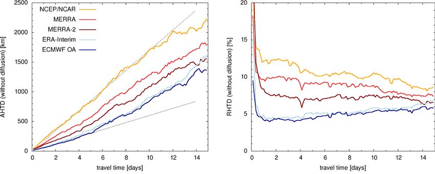
490       SPARC Reanalysis Intercomparison Project (S-RIP) Final Report                                                           -- Early online release --

                                                                                                                                                         Contents
  10.1 Introduction...............................................................................................................................................491
  10.2 Description of Atmospheric Measurements..........................................................................................493
     10.2.1 Aura Microwave Limb Sounder.......................................................................................................493
     10.2.2 Envisat MIPAS....................................................................................................................................494
     10.2.3 CALIPSO CALIOP............................................................................................................................494
     10.2.4 COSMIC GNSS-RO...........................................................................................................................494
     10.2.5 Concordiasi Superpressure Balloon Measurements......................................................................495
  10.3 Overview of Reanalysis Polar Temperature Differences.......................................................................496
  10.4 Polar Temperature and Vortex Diagnostics...........................................................................................496
  10.5 Polar Diabatic Heating Rates.................................................................................................................. 500
  10.6 Concordiasi Superpressure Balloon Comparisons................................................................................503
     10.6.1 Temperatures and Winds..................................................................................................................503
     10.6.2 Trajectories.........................................................................................................................................504
  10.7 PSC Thermodynamic-Consistency Diagnostics....................................................................................505
     10.7.1 Mountain Waves................................................................................................................................505
     10.7.2 Thermodynamic Equilibrium...........................................................................................................506
     10.7.3 Temperature Difference Profiles.......................................................................................................507
     10.7.4 Summary of the Temperature Differences......................................................................................508
  10.8 Chemical Modeling Diagnostics.............................................................................................................508
     10.8.1 Details of the BASCOE System and Experimental Setup..............................................................509
     10.8.2 Analysis Approach.............................................................................................................................510
     10.8.3 Case Study: 2009 Antarctic Winter..................................................................................................510
     10.8.4 Case Study: 2009/2010 Arctic Winter..............................................................................................517
     10.8.5 Comparisons of Chemical Ozone Loss...........................................................................................518
     10.8.6 Discussion and Implications.............................................................................................................519
  10.9 Summary, Key Findings, and Recommendations.................................................................................520
  References..............................................................................................................................................................524
  Major abbreviations and terms...........................................................................................................................529

                                                                       -- Early online release --
-- Early online release --                                                       Chapter 10: Polar Processes           491

10.1   Introduction                                             and in the autumn and spring in the Antarctic. As noted,
                                                                for example, by Hoffmann et al. (2017a) and Lambert and
                                                                Santee (2018) and discussed further below, in addition to
One of the main research themes in atmospheric science          discrepancies in physical parameters (e.g., temperature,
over the past three decades has been the investigation of the   winds) between the various reanalyses, differences in their
chemical and dynamical processes involved in stratospher-       temporal and/or spatial resolution may also play a role in
ic ozone depletion, the most severe manifestation of which      detailed quantitative studies.
is the Antarctic ozone hole. In general, the processes con-
trolling polar stratospheric ozone are now well understood      Given the importance of stratospheric temperatures, trans-
(e.g., WMO, 2018). In the very cold conditions that prevail     port, and mixing for ozone chemistry, a number of studies
inside the lower stratospheric winter polar vortices, water     over the last twenty years have assessed the representative-
vapour (H2O) and nitric acid (HNO3) condense to form            ness of meteorological analyses and reanalyses. We briefly
polar stratospheric clouds (PSCs). PSC particles and cold       summarize here several studies that carried out compar-
sulphate aerosols provide surfaces on which heterogeneous       isons of two or more analyses/reanalyses specifically in a
reactions can take place very rapidly, converting chlorine      stratospheric polar processing framework. In one of the
from relatively benign reservoir species such as hydrogen       earliest such studies, Manney et al. (1996) examined tem-
chloride (HCl) and chlorine nitrate (ClONO2) into highly        peratures, geopotential heights, winds, and potential vor-
reactive ozone-destroying forms such as chlorine monox-         ticity (PV) calculated from stratospheric analyses provided
ide (ClO). Moreover, sequestration in PSCs substantial-         by the (then) UK Meteorological Office (UKMO) and the
ly reduces gas-phase HNO3 concentrations, and if solid          US National Meteorological Center (NMC) in both hemi-
HNO3-containing PSC particles grow large enough to un-          spheres during dynamically active periods, when substan-
dergo appreciable gravitational sedimentation, then HNO3        tial discrepancies between analyses were likely to be seen.
can be irreversibly removed from the stratosphere in a pro-     Although both analyses captured the qualitative features
cess known as denitrification. Similarly, sedimentation of      and evolution of the large-scale winter stratospheric circu-
water ice particles leads to dehydration. Severe denitrifica-   lation, differences in their temperatures and polar vortex
tion and dehydration routinely occur in the cold, isolated      characteristics implied significant effects on quantitative
Antarctic vortex. Compared to the Antarctic, the Arctic         process studies, especially for the Southern Hemisphere.
vortex is usually substantially warmer, more dynamically        Knudsen (1996) also found substantial biases between
disturbed, smaller, and shorter lived, and thus in a typical    observed lower stratospheric temperatures and analyses
year it experiences little or no denitrification or dehydra-    from UKMO and the European Centre for Medium-range
tion. Chlorine activation is also typically less intense, ex-   Weather Forecasts (ECMWF). Knudsen et al. (2001) as-
tensive, and prolonged in the Arctic than in the Antarctic.     sessed the accuracy of analyzed winds from ECMWF,
Consequently, although the same fundamental processes           UKMO, and the US National Centers for Environmental
are at work in the lower stratosphere in both polar regions,    Prediction (NCEP) Climate Prediction Center (CPC) by
in most years chlorine-catalyzed ozone loss is considerably     comparing calculated air parcel trajectories based on those
weaker in the Arctic than in the Antarctic.                     analyses with long-duration balloon flights in the Arctic
                                                                stratospheric vortex. Similarly, Knudsen et al. (2002) used
Lower stratospheric polar processes and chemical ozone          independent meteorological measurements from long-du-
loss are “threshold” phenomena that depend critically on        ration balloon flights in the Arctic stratospheric vortex
stratospheric temperatures and other meteorological and         to quantify errors in five sets of analyzed temperatures:
dynamical factors (e.g., winter polar vortex characteristics,   ECMWF, Met Office (formerly UKMO), the Goddard Space
breakup dates, etc.). Several studies over the years have ex-   Flight Center Data Assimilation Office (DAO), NCEP/CPC,
plored the temperature sensitivity of these processes; for      and NCEP/National Center for Atmospheric Research re-
example, Wegner et al. (2012) showed that heterogeneous         analysis (NCEP-NCAR R1); although some of the analy-
reaction rates on liquid aerosols are doubled for every 1 K     ses showed larger scatter around the balloon values than
in cooling and increase tenfold over a 2-K range around         others, occasional large differences occurred in all of them,
192 K, and Solomon et al. (2015, see also references therein)   particularly during a major sudden stratospheric warming.
showed that a 2-K perturbation in temperature applied to        Manney et al. (2003b) compared commonly used meteoro-
heterogeneous chemical reactivities and PSC surface area        logical analyses (Met Office, NCEP/CPC, NCEP-NCAR R1,
in a specified-dynamics chemistry climate model induces         ECMWF, DAO) during two cold Arctic winters, examin-
a change in simulated Arctic column ozone loss of ~ 40 DU.      ing not only temperatures (average and minimum values,
                                                                number of cold days, etc.) but also temperature histories
As in many other Earth system science specialties, atmos-       along trajectories to assess simulated PSC lifetimes and the
pheric polar processing studies often rely heavily on glob-     overall potential for chlorine activation. They found that
al meteorological data sets. Thus it is essential to under-     discrepancies between analyses arise from differences in
stand the accuracy and reliability of reanalysis fields in a    both the magnitude and the morphology of wind and tem-
polar processing context. Differences between reanalyses        perature fields, such that dissimilarities in dynamical con-
are likely to have the largest impact on such studies when      ditions in comparably cold winters may strongly influence
conditions are marginal, i.e., in the Arctic (in most years)    the degree of agreement between meteorological data sets.

                                                    -- Early online release --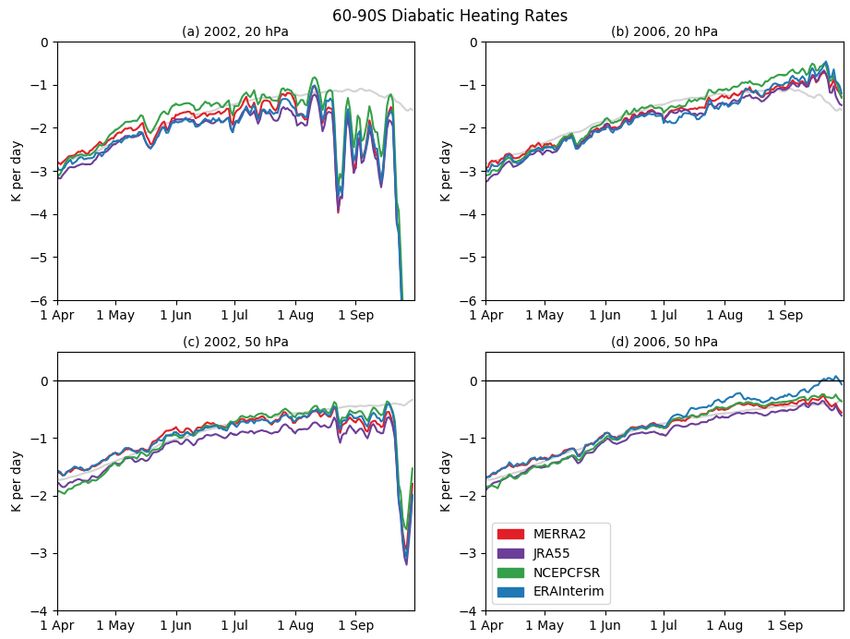
492     SPARC Reanalysis Intercomparison Project (S-RIP) Final Report                     -- Early online release --

Following on from that study, Manney et al. (2005) in-         of the ozone hole during the highly disturbed Antarctic
vestigated an extensive set of diagnostics related to lower    winter of 2002; although runs driven by both analyses
stratospheric chemistry, transport, and mixing during          reproduced the anomalous conditions in that winter,
the 2002 Antarctic winter, when unusual dynamical              differences in the structure and magnitude of simulated
activity may have exacerbated the disagreement be-             total ozone were seen.
tween meteorological data sets. Comparing four oper-
ational products (Met Office, ECMWF, NCEP/CPC, and             Lawrence et al. (2015) revisited the use of polar pro-
the NASA Global Modeling and Assimilation Office               cessing diagnostics to evaluate reanalyses, performing
(GMAO) Goddard Earth Observing System (GEOS-4)),               a comprehensive intercomparison of NASA’s Modern
as well as the 40-year reanalysis from ECMWF (ERA-             Era Retrospective-analysis for Research and Applica-
40), NCEP-NCAR R1, and a second NCEP/Department                tions (MERRA) and ERA-Interim over the period 1979
of Energy reanalysis (NCEP-DOE R2), they again found           to 2013. Agreement between the two meteorological data
considerable differences; such large disparities under-        sets changed substantially during this interval, with
mine confidence in the results from scientific studies         many stratospheric temperature and vortex characteris-
based on any of those analyses/reanalyses. In particu-         tics converging to greater consistency over time as more
lar, NCEP-NCAR R1, NCEP-DOE R2, and ERA-40 were                high-quality observations were assimilated. Lawrence
shown to suffer from substantial deficiencies in their de-     et al. (2015) concluded that for the years since 2002 the
piction of the magnitude, structure, or evolution of tem-      MERRA and ERA-Interim reanalyses are equally appro-
peratures and/or winds that rendered them unsuitable           priate choices and either can be used with confidence in
for detailed studies of lower stratospheric polar process-     polar processing studies in both hemispheres. In a fol-
ing. Labitzke and Kunze (2005) compared stratospheric          low-up study, Lawrence et al. (2018) extended the applica-
temperatures over the Arctic from NCEP-NCAR R1 and             tion of polar processing diagnostics to encompass other
ERA-40 with an independent data set (historical daily          current full-input reanalyses, including MERRA-2, the
analyses of Northern Hemisphere temperature fields             Japanese 55-year Reanalysis (JRA-55), and the NCEP
over 100 - 10 hPa produced by hand at FU Berlin); al-          Climate Forecast System Reanalysis / Climate Forecast
though agreement in the long-term mean temperatures            System, version 2 (CFSR/CFSv2). Results from this later
and the trends (1957 - 2001) was generally good, they          study are described in detail in Section 10.4.
also found unrealistic behavior in ERA-40, which dis-
played larger biases in the October to January interval        In summary, several previous studies have found consid-
after 1979. Tilmes et al. (2006) focused specifically on the   erable discrepancies between meteorological analyses/
volume of air below the temperature threshold for PSC          reanalyses in various parameters of relevance for polar
existence (VPSC); they found that, although the general        processing, revealing that significant quantitative and
patterns of VPSC evolution were similar for Met Office         qualitative differences may arise from the choice of which
and ERA-40 reanalyses as well as ECMWF operational             meteorological products are used in a given study. The
analyses and data from FU-Berlin, differences between          recent work of Lawrence et al. (2015, 2018) indicates that
the two reanalyses were as large as 10 % during their pe-      agreement among various modern reanalyses improved
riod of overlap (1991 - 1999). Rieder and Polvani (2013)       substantially for some polar processing diagnostics in the
also touched on comparisons of VPSC , computing it us-         post-2001 timeframe, following the introduction of new
ing temperatures from MERRA, ECMWF Interim Rea-                data streams. Nevertheless, previous studies have not
nalysis (ERA-Interim), and NCEP-NCAR R1. Although              examined all reanalyses of interest for S-RIP; moreover,
the depiction of year-to-year variability was seen to be       a comparison of metrics not explored in earlier papers
strongly correlated among the three reanalyses, the mag-       would be informative. Thus a comprehensive reassess-
nitude of VPSC varied considerably, with MERRA and             ment is warranted.
ERA-Interim indicating VPSC values roughly 30 % larger
than those from NCEP-NCAR R1. Rieder and Polvani               In this chapter we intercompare recent full-input reanal-
reiterated the cautions raised earlier about using NCEP-       yses using an extensive set of polar processing diagnos-
NCAR R1 in detailed polar processing studies.                  tics. The specific reanalyses considered here are: MERRA,
                                                               MERRA-2, ERAInterim, JRA-55, and CFSR/CFSv2. Fuji-
A few studies have looked at the impact of differences         wara et al. (2017) provide an overview of these reanalysis
in meteorological fields on results from chemical trans-       systems, and they are also described in detail in Chap-
port models (CTMs). Davies et al. (2003) investigated          ter 2 of this Report. We note that ECMWF stopped pro-
the effects of denitrification on ozone depletion in a         ducing ERA-Interim in August 2019 and replaced it with
cold Arctic winter by forcing a 3D CTM incorporating           ERA5. Because the bulk of the analysis for this chapter
different PSC schemes with both UKMO and ECMWF                 had already been completed by the time ERA5 became
analyses, finding that the two meteorological data sets        available, its performance has not been assessed here.
led to disparate patterns of modeled PSC formation and         Although we expect that ERA5 will prove to be at least
denitrification, and consequently also chlorine activa-        as reliable for polar processing studies as other modern
tion and ozone loss. Similarly, Feng et al. (2005) applied     reanalyses, we can make no conclusive judgments about
the same CTM and analyses to examine the evolution             its suitability for such studies at this time.

                                                   -- Early online release --
-- Early online release --                                                         Chapter 10: Polar Processes            493

The primary focus here is on reanalyses; however, in some         the spatially and temporally varying differences between
cases where comparisons with atmospheric observations             reanalyses and exemplify how their net effects impact the
are made we also examine the ECMWF operational analy-             bottom-line conclusions of typical real-life studies, in Sec-
sis (OA) and the NASA GMAO Goddard Earth Observing                tion 10.8 we compare simulated sequestration of HNO3 and
System Version 5.9.1 (GEOS-591) assimilation product. The         H2O in PSCs, chlorine activation, and ozone fields with
ECMWF OA evaluated by Hoffmann et al. (2017a), whose              those observed by Aura MLS and the Envisat Michelson
results are summarized in Section 10.6, is characterized by       Interferometer for Passive Atmospheric Sounding (MIP-
3-hr temporal resolution, 0.125 ° × 0.125 ° horizontal resolu-    AS) for one winter in each hemisphere. Model-based esti-
tion, and 91 vertical levels with an upper lid at 0.01 hPa. The   mates of Antarctic chemical ozone loss in the stratospheric
GEOS-591 near-real-time analysis, which was produced by           partial column are also compared with those derived from
the GEOS-5 data assimilation system (Molod et al., 2015; Rie-     MLS data. Other commonly used ozone loss metrics such
necker et al., 2011), was characterized by 3-hr temporal res-     as ozone hole area, ozone mass deficit, etc., are not includ-
olution, 0.625 ° × 0.5 ° horizontal resolution, and 72 vertical   ed here, nor are other processes that affect polar ozone but
levels with an upper lid at 0.01 hPa. This stable system, used    that are covered extensively elsewhere in this Report (e.g.,
by NASA Earth Observing System satellite instrument teams         sudden stratospheric warmings are discussed in Chapter 6).
in their data processing, provided consistent meteorological      Further direct comparisons between observations and the
fields over much of the Aura record and was thus somewhat         ozone fields from the reanalyses can be found in Chapter 4.
akin to a reanalysis. It was assessed by Lambert and San-
tee (2018), whose results are summarized in Section 10.7.
                                                                  10.2 Description of Atmospheric Measurements
Much of this chapter focuses on process-oriented and case
studies. For many diagnostics, the degree of agreement
between reanalyses is an important direct indicator of the        10.2.1 Aura Microwave Limb Sounder
systems’ inherent uncertainties, for which comparisons to
independent measurements are not required. In addition,           MLS measures millimeter- and submillimeter-wavelength
some diagnostics are based on PV or other dynamical quan-         thermal emission from the limb of Earth’s atmosphere
tities that cannot be provided directly by any measurement        (Waters et al., 2006). The Aura MLS field-of-view (FOV)
system. These situations pertain to many of the polar tem-        points in the direction of orbital motion and vertically
perature and vortex diagnostics presented in Section 10.4,        scans the limb in the orbit plane, providing data cover-
including minimum lower stratospheric temperature, area           age from 82 ° S to 82 ° N latitude on every orbit. Because
and volume of stratospheric air with temperatures below           the Aura orbit is sun-synchronous (with a 13:45 local time
PSC existence thresholds, maximum latitudinal gradients           ascending equator-crossing time), MLS observations at
in PV (a measure of the strength of the winter polar vortex),     a given latitude on either the ascending (mainly day) or
area of the vortex exposed to sunlight each day, and vortex       descending (mainly night) portions of the orbit have the
breakup dates, as well as the polar cap average diabatic heat-    same local solar time. Northern high latitudes are sam-
ing rates discussed in Section 10.5. On the other hand, com-      pled by ascending measurements near midday local time,
parisons with atmospheric measurements can be made for            whereas southern high latitudes are sampled by ascending
some diagnostics, especially the more derived ones. Such          measurements in the late afternoon. Vertical profiles are
comparisons typically demand fairly broad spatial coverage        measured every ~ 165 km along the suborbital track, yield-
on a daily basis, which is best afforded by satellite measure-    ing a total of ~ 3500 profiles per day.
ments. For the most part, comparisons between reanalysis
fields and independent observations are left to Chapter 3;        Here, we use the MLS version 4.2 (v4.2) data (Livesey et
Long et al. (2017) also presented comparisons of reanaly-         al., 2020). Detailed information on the quality of a previ-
sis temperatures against satellite observations. However,         ous version of MLS data, v2.2, can be found in dedicated
analyses/reanalyses are evaluated through comparisons             validation papers by Lambert et al. (2007) for stratospher-
with long-duration superpressure balloon temperature and          ic H2O, Santee et al. (2007) for HNO3, Santee et al. (2008)
wind measurements in Section 10.6. In addition, the Con-          for ClO, Froidevaux et al. (2008a) for HCl, Froidevaux
stellation Observing System for Meteorology, Ionosphere           et al. (2008b) for stratospheric O3, and Schwartz et al.
and Climate (COSMIC) global navigation satellite system           (2008) for temperature. The precision, resolution, and
(GNSS) radio occultation (RO) temperatures are exam-              useful vertical range of the v4.2 measurements, as well
ined in connection with PSC thermodynamic-consistency             as assessments of their accuracy through systematic error
diagnostics in Section 10.7. The latter section also relies on    quantification (and, in some cases, validation compari-
vertical profiles of gas-phase HNO3 and H2O measured by           sons with correlative data sets), are reported for each spe-
the Aura Microwave Limb Sounder (MLS), as well as PSC             cies by Livesey et al. (2020). Briefly, MLS measurements
characteristics determined from Cloud-Aerosol Lidar and           have single-profile precisions (accuracies) of 4 - 15 %
Infrared Pathfinder Satellite Observations (CALIPSO)              (4 - 20 %) for H2O, 0.6 ppbv (1 - 2 ppbv) for HNO3, 0.1 ppbv
Cloud-Aerosol Lidar with Orthogonal Polarization (CALI-           (0.05 - 0.25 ppbv) for ClO, 0.2 - 0.3 ppbv (0.2 ppbv) for HCl,
OP) lidar aerosol and cloud backscatter. Finally, because re-     0.05 - 0.1 ppmv (0.1 - 0.25 ppmv) for O3, and 0.6 - 1.2 K
sults from chemical models synthesize the interplay among         (0 - 5 K) for temperature in the stratosphere.

                                                      -- Early online release --
494     SPARC Reanalysis Intercomparison Project (S-RIP) Final Report                       -- Early online release --

We note that MERRA-2 assimilates MLS temperatures,              below 40 km, precision is 8 - 14 %, with vertical resolution
but only at pressures less than 5 hPa and not within the        2.5 - 9 km (Höpfner et al., 2007; von Clarmann et al., 2009).
pressure range investigated here (Gelaro et al., 2017).         Retrieval of ClONO2 is hindered by the presence of opti-
                                                                cally thick PSCs along the MIPAS line of sight.
Errors in the MLS H2O contribute a few tenths of a kelvin
to the error in calculated frost point temperatures and are
substantially smaller than the errors in the temperature        10.2.3 CALIPSO CALIOP
limb sounding retrievals obtained from MLS. From Au-
gust 2004 until December 2013, mean differences between         The CALIOP dual-wavelength elastic backscatter lidar
NOAA frost point hygrometer and MLS H2O data showed             (Winker et al., 2009) flies on the Cloud-Aerosol Lidar
no statistically significant differences (agreement to better   and Infrared Pathfinder Satellite Observations (CALIP-
than < 1 %) from 68 - 26 hPa, although significant biases       SO) satellite launched in April 2006. We use the CAL-
at 100 hPa and 83 hPa were found to be 10 % and 2 %, re-        IOP Level 2 operational data set L2PSCMask (v1 Polar
spectively (Hurst et al., 2014). However, increasing the time   Stratospheric Cloud Mask Product) produced by the CA-
frame to mid-2015 revealed a long-term drift in MLS H2O         LIPSO science team. The Level 2 operational data con-
of up to 1.5 % per year starting around 2010 (Hurst et al.,     sist of nighttime-only data and contain profiles of PSC
2016). Although changes to the MLS data processing system       presence, composition, optical properties, and meteoro-
have substantially mitigated this drift in the version 5 MLS    logical information along the CALIPSO orbit tracks at
H2O measurements, for the v4 data used here the effect on       a horizontal resolution of 5 km and a vertical resolution
the calculated supercooled ternary solution (STS) reference     of 180 m. We have applied post-processing to generate
and frost point temperatures is less than 0.1 K per year.       coarser horizontal/vertical bins for a better comparison
                                                                at the scale of the MLS along-track and vertical resolu-
To aid in the analysis of MLS measurements, particularly        tion (see Section 10.7 for details). Each averaging bin is
in Section 10.7, we make use of MLS Derived Meteoro-            the size of the MLS along-track vertical profile separa-
logical Products (DMPs). These files contain meteorolog-        tion (165 km) and the height between the mid-points of
ical data (e.g., temperature) and derived parameters (e.g.,     the retrieval pressure levels (2.16 km) for the MLS HNO3
equivalent latitude) interpolated from gridded reanalysis       data product. This we refer to as the MLS geometric FOV.
fields to the along-track geolocations of the MLS meas-         There are approximately four hundred 5 km × 180 m
urements. The original version of the MLS DMPs was              CALIOP “pixels” within the MLS geometric FOV.
described in detail by Manney et al. (2007). Here we use
updated files (version 2, the DMP version of record for         The CALIOP PSC classification scheme used here is de-
the MLS v4.2 data; see the MLS web page, http://mls.jpl.        scribed by Pitts et al. (2009), with modifications discussed
nasa.gov, for more details); the v2 DMPs are from the           by Pitts et al. (2013), and consists of four main PSC types.
software described by Manney et al. (2011a). DMP files          MIX1 and MIX2 denote detections of nitric acid trihydrate
containing associated meteorological information at the         (NAT) particles, with the MIX1/MIX2 boundary marking
MLS measurement locations have been produced for all            a transition between lower (MIX1) and higher (MIX2)
five full-input reanalyses considered here.                     NAT number/volume densities. The STS type indicates
                                                                supercooled liquid ternary solution (H2SO4/HNO3/H2O)
                                                                particles, and ICE indicates water-ice particles.
10.2.2 Envisat MIPAS

The MIPAS instrument (Fischer et al., 2008) was launched        10.2.4 COSMIC GNSS-RO
in March 2002 on the ESA Environment Satellite (Envi-
sat) and was operational until April 2012. MIPAS was an         We use the US/Taiwan Constellation Observing System for
infrared Fourier transform spectrometer for measuring           Meteorology, Ionosphere and Climate (COSMIC) network
limb emission spectra between 685 cm-1 and 2410 cm-1            data obtained from the Universities for Cooperative At-
(14.6 - 4.15 µm). Through azimuth scanning it provided          mospheric Research (UCAR) COSMIC Data Analysis and
global coverage from 87.5 ° S to 89.3 ° N. The instrument       Archive Center (CDAAC). Global navigation satellite sys-
FOV was 30 km across-track and 3 km in the vertical, and        tem radio occultation (GNSS-RO) data have provided high
the horizontal along-track sampling distance for nomi-          accuracy (bias < 0.2 K and precision > 0.7 K, Gobiet et al.,
nal-mode observations was ~ 530 km from 2002 to 2004            2007), global (day and night) coverage, coupled with ex-
and ~ 400 km from 2005 onward. Several retrieval algo-          cellent long term stability, for nearly two decades (Anthes,
rithms have been developed for the MIPAS spectra; here          2011). The vertical resolution is better than about 0.6 km
we use profiles of temperature and atmospheric constitu-        over the 15 - 30 km vertical range considered here. The in-
ents generated by the KIT-IMF-ASF (Karlsruhe Institute          troduction of GNSS-RO has been documented to improve
of Technology, Institute of Meteorology and Climate Re-         numerical weather prediction (NWP) forecast skill in
search, Atmospheric Trace Gases and Remote Sensing)             the ECMWF Integrated Forecast System (IFS) (Bonavita,
group in cooperation with the Instituto de Astrofísica          2014) and to reduce tropopause and lower stratospher-
de Andalucía (von Clarmann et al., 2009). For ClONO2            ic temperature biases in ERA-Interim (Poli et al., 2010).

                                                    -- Early online release --
-- Early online release -- Chapter 10: Polar Processes 495
The direct assimilation of bending angles or refractivity Concordiasi was equipped with a meteorological pay-
is now the common practice for many global reanaly- load called the Thermodynamical SENsor (TSEN).
ses; however, for many other purposes the production of TSEN makes in situ measurements of atmospheric pres-
vertical atmospheric temperature profiles from GNSS- sure and temperature every 30 s during the whole flight.
RO data is required. The retrieval of vertical atmos- The pressure is measured with an accuracy of 1 Pa and
pheric geophysical profiles from RO requires a number a precision of 0.1 Pa. The air temperature is measured
of assumptions because of the long ray path through a via two thermistors. During daytime, the thermistors
non-uniform atmosphere (Ho et al., 2012). Therefore, are heated by the sun, leading to daytime temperature
corrections are required for ionospheric effects, vari- measurements being warmer than the real air tempera-
ations in water vapour, and gradients in temperature ture. An empirical correction has been used to correct
along the ray path (Anthes, 2011; Poli and Joiner, 2004). for this effect, which is described in detail by Hertzog et
Many other studies have intercompared GNSS-RO with al. (2004). The precision of the corrected temperature
independent operational analyses, e.g., with forecast observations is about 0.25 K during daytime and 0.1 K
versions that have not assimilated the GNSS-RO data. during nighttime.
The near real time COSMIC data (in the form of bend-
ing angles or refractivity) are ingested by most of the Most of the measurements (i.e., more than 90 %) took
data assimilation procedures considered here (except for place between 25 September and 22 December 2010,
MERRA), and therefore these reanalyses are not strictly at an altitude range of 17.0 - 18.5 km, and within a lat-
independent of the postprocessed COSMIC tempera- itude range of 59 - 84 ° S. The pressure measurements
tures. We have chosen to use the COSMIC temperatures are mostly within a range of 58.2 - 69.1 hPa and the
as a common reference to evaluate the reanalysis depar- temperature measurements within 189 - 227 K. The
tures, rather than using the reanalysis ensemble mean. density of air, calculated from pressure and tempera-
ture, varies between 0.099 kg m-3 and 0.120 kg m-3. The
zonal winds are predominately westerly and mostly
10.2.5 Concordiasi Superpressure Balloon Measurements within a range of 1 - 44 m s -1. The meridional wind
distributions are nearly symmetric, with meridional
Superpressure balloons are aerostatic balloons, which winds being in the range of ± 17 m s -1. Horizontal wind
are filled with a fixed amount of lifting gas, and for speeds are mostly within 5 - 47 m s -1.
which the maximum volume of the balloon is kept con-
stant by means of a closed, inextensible, spherical enve- The Concordiasi balloon observations have been assim-
lope. After launch, the balloons ascend and expand un- ilated into the ECMWF, MERRA, and MERRA-2 data
til they reach a float level where the atmospheric density sets, but they were not considered for NCEP-NCAR R1.
matches the balloon density. On this isopycnic surface The observations therefore provide an independent data
a balloon is free to float horizontally with the motion source only for the validation of the NCEP-NCAR R1
of the wind. Hence, superpressure balloons behave as data set. However, as meteorological analyses are a re-
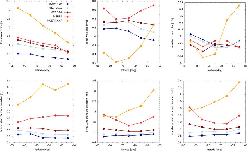
quasi-Lagrangian tracers in the atmosphere. The Con- sult of combining various satellite and in situ observa-
cordiasi field campaign in Antarctica in September tions, a forecast model, and a data assimilation proce-
2010 to January 2011 was aimed at making innovative dure, a comparison of the meteorological data with the
atmospheric observations to study the circulation and Concordiasi observations still provides information on
chemical species in the polar lower stratosphere and to the performance of the overall system, even for the rea-
reduce uncertainties in diverse fields in Antarctic sci- nalyses that assimilate those observations. As the obser-
ence (Rabier et al., 2010). During the field campaign, vational data have been subject to downsampling and
19 superpressure balloons with 12 m diameter were data thinning before they were assimilated, an assess-
launched from McMurdo Station (78 ° S, 166 ° E), Ant- ment of the representation of small-scale structures due
arctica, by the French space agency, Centre National to gravity waves also remains meaningful.
d’Etudes Spatiales (CNES). Balloons of this size typi-
cally drift at pressure levels of ~ 60 hPa and altitudes of Trajectory calculations for the Concordiasi balloon
~ 18 km. The balloons were launched between 8 Septem- observations have been analyzed using the Lagrangi-
ber and 26 October 2010, and each balloon flew in the an particle dispersion model Massive-Parallel Trajec-
mid- and high-latitude lower stratosphere for a typical tory Calculations (MPTRAC) (Hoffmann et al., 2016).
period of 2 to 3 months. Transport is simulated by calculating trajectories for
large numbers of air parcels based on given wind fields
The positions of the balloons were tracked every 60 s by from global meteorological reanalyses. The numerical
means of global positioning satellite (GPS) receivers. At accuracy and efficiency of trajectory calculations with
each observation time the components of the horizon- MPTRAC was assessed by Rößler et al. (2018). Turbulent
tal wind are computed by finite differences between the diffusion and subgrid-scale wind fluctuations are sim-
GPS positions. The uncertainty is about 1 m for the GPS ulated based on the Langevin equation, closely follow-
horizontal position and 0.1 m s -1 for the derived winds ing the approach implemented in the Flexible Particle
(Podglajen et al., 2014). Each balloon launched during (FLEXPART) model (Stohl et al., 2005).
-- Early online release --496 SPARC Reanalysis Intercomparison Project (S-RIP) Final Report -- Early online release --
10.3 Overview of Reanalysis Polar Temperature Differences the same magnitude. Indeed, whereas Hoffmann et al.
(2017a) find MERRA to be the warmest and ERA-Interim
the coldest compared to superpressure balloon temper-
To provide context for later results derived from more ature measurements made during the Antarctic Con-
complex analysis techniques, we show in Figure 10.1 a cordiasi campaign in September 2010 to January 2011,
basic overview of reanalysis temperatures in the polar Lambert and Santee (2018) find the opposite order com-
lower stratosphere. We have chosen as a suitable metric pared to the COSMIC and thermodynamic temperature
the daily (12 UT) mean 60 ° polar cap temperature dif- references for May to August during 2008 to 2013. To
ferences at 46 hPa. Time series of the temperature differ- reconcile this apparent discrepancy, in Figure 10.2 dai-
ences calculated for MERRA, MERRA-2, JRA-55, and ly mean temperature differences (at 12 UT) for MERRA
CFSR/CFSv2 relative to ERA-Interim over 2008 - 2013 and MERRA-2 relative to ERA-Interim are used to high-
have been smoothed using a 10-day boxcar average. The light the non-overlapping intervals of the PSC analysis
daily mean standard error of the temperature differences window (green line) and the balloon flights (red line).
is less than 0.1 K. In both hemispheres, temperature dif- Measurements in the later time period of the Concordia-
ferences display annual cycles, with positive deviations si balloon flights (September - December) clearly sample
mainly in summer and negative deviations mainly in different atmospheric conditions than those prevailing in
winter. In the Antarctic the largest deviations are ~ 1 K in the earlier time period (May - August). Moreover, differ-
MERRA − ERA-Interim, whereas in the Arctic the largest ences between reanalysis temperatures along individual
deviations are in JRA-55 − ERA-Interim, but they only balloon trajectories are likely to be amplified compared
reach ~ 0.5 K. to the differences in mean polar cap temperatures. We
note that MERRA does not assimilate COSMIC data,
The grey-shaded regions in Figure 10.1 mark the use- whereas MERRA-2 and the other reanalyses investigated
ful wintertime measurement periods, chosen to capture here do; hence some of the reduction in the bias of MER-
the bulk of the PSC activity needed for the evaluation of RA-2 compared to MERRA seen in Figure 10.2 is likely
the thermodynamic temperature comparisons that are attributable to the former’s use of GNSS-RO data.
discussed in Section 10.7. These periods also happen to
largely coincide with times of smaller variability in the
temperature differences, when biases of the other rea- 10.4 Polar Temperature and Vortex Diagnostics
nalyses with respect to ERA-Interim are predominantly
negative. Therefore, we caution that intercomparisons of Lawrence et al. (2018) expanded on the diagnostics in
reanalyses undertaken using other time periods, espe- Lawrence et al. (2015) and applied them to CFSR/CFSv2,
cially for summertime, could even obtain temperature ERA-Interim, JRA-55, and MERRA-2 (evaluations were
deviations of opposite sign whilst maintaining about also done for MERRA but were not included in the paper).
Figure 10.1: (a) Time series (for 12 UT) from 2008 to 2013 of 10-day boxcar-smoothed temperature differences for MERRA, MERRA-2,
JRA-55, and CFSR/CFSv2 relative to ERA-Interim at 46 hPa, averaged over the 60 ° Antarctic polar cap. The four reanalyses being dif-
ferenced against ERA-Interim are shown in the colors indicated in the legend between the two panels. Grey regions indicate the pe-
riods defined for the analysis of PSC-related metrics (see Section 10.7). (b) Same, but for the Arctic. From Lambert and Santee (2018).
-- Early online release ---- Early online release -- Chapter 10: Polar Processes 497
Figure 10.2: Daily mean temperature differences (grey) of (a) MERRA and (b) MERRA-2, relative to ERA-Interim at 62 hPa (repre-
sentative of the Concordiasi balloon float heights (see Section 10.6) in the 60 ° Antarctic polar cap for 2008 - 2013. The green-black
dashed line indicates the mean of the 2008 - 2013 differences (green symbols) during the PSC analysis window. The red-black dashed
line indicates the mean of the differences (red symbols) over the time span of 90 % of the Concordiasi balloon measurements in 2010
(Hoffmann et al., 2017a). From Lambert and Santee (2018).
The full suite of diagnostics examined by Lawrence et al. agree with the REM to within about 0.5 K in the most re-
(2018) includes minimum temperatures poleward of ± 40 ° cent decade, though differences in the early years common-
latitude, the areas of temperatures (poleward of ± 30 ° lat- ly exceed 3 K. The standard deviations of the differences
itude) below PSC existence thresholds, the winter mean increase with altitude (indicating larger maximum differ-
volume of lower stratospheric air with temperatures be- ences between the reanalyses) and show a modest decrease
low PSC existence thresholds, maximum gradients in over the time period, with an abrupt decrease seen around
scaled PV as a function of equivalent latitude, the area of 1998 in most reanalyses. CFSR/CFSv2 generally shows larg-
the vortex exposed to sunlight, and approximate dates of er variance than the other reanalyses in the period since
the breakup of the polar vortices. As noted by Lawrence et about 2002, and less of a change around 1998. These fea-
al. (2018), reanalysis comparisons are particularly critical tures are consistent with those from comparisons of other
to assess the uncertainties in these types of diagnostics be- polar processing diagnostics. In the Northern Hemisphere
cause they are not quantities that can be compared directly (NH), the reanalyses agree much better throughout the 36
with observations. The key results of Lawrence et al. (2018) years (to within about 1.5 K before 1999), though conver-
are summarized below. gence toward better agreement is also seen in most of the
reanalyses (excepting CFSR/CFSv2) (Lawrence et al., 2018);
Figure 10.3 compares Southern Hemisphere (SH) extended this is not unexpected since the input data density (from,
winter season (MJJASO) minimum temperatures poleward e.g., sondes and ground-based measurements) in the years
of 40 ° S in the lower stratosphere from MERRA-2, ERA-In- before the TOVS/ATOVS transition was much greater in
terim, JRA-55, and CFSR/CFSv2 with those from the rea- the NH, and thus the reanalyses’ temperatures before that
nalysis ensemble mean (REM). Since the REM values that transition were much better constrained than those in the
go into each season’s mean vary from day to day and are ex- SH. Lawrence et al. (2018) also evaluated the area of temper-
pected to change with any large change in any of the reanal- atures below PSC thresholds, with results consistent with
yses, the differences from the REM quantify only how far those shown here for minimum temperatures.
each reanalysis is from that mean during each season, thus
giving an idea of the range of values (which could be inter- Figure 10.4 shows differences from the REM of daily max-
preted as an uncertainty in the diagnostic) but not of the imum PV gradients (a measure of vortex strength) with
absolute changes in those values. The standard deviations respect to equivalent latitude averaged over the DJFM
shown on the right of Figure 10.3 help further quantify the season in the NH, as well as the standard deviations of
spread among the reanalyses. The reanalyses converge to- the daily differences. The climatological maximum val-
wards much better agreement in the later years at all levels. ues of this diagnostic increase with height from around
There are step-like changes in agreement among the reanal- 1 - 6 × 10⁻⁶ s-1 deg-1 at about 430 K to over 20 × 10-6 s-1 deg-1
yses around 1998 (especially ERA-Interim and MERRA-2), above about 600 K (Lawrence et al., 2018). There is no
when the reanalyses (albeit not all at exactly the same time) obvious systematic decrease in the differences from the
changed from assimilating Tiros Operational Vertical REM, and a very slight apparent decrease in the standard
Sounder (TOVS) to advanced TOVS (ATOVS) radiances; deviations for most reanalyses. Not shown is a small sys-
the latter provide higher-resolution constraints on strato- tematic decrease in the difference between MERRA and
spheric temperatures. On average, the individual reanalyses MERRA-2 for a narrow range of levels from 580 K to 700 K.
-- Early online release --498 SPARC Reanalysis Intercomparison Project (S-RIP) Final Report -- Early online release --
Minimum Temperatures: Differences from REM (SH, MJJASO period)
(a) CFSR/CFSv2 Mean Diffs (b) CFSR/CFSv2 StdDev of Diffs
10 10
14.7 14.7
Pressure [hPa]
Pressure [hPa]
21.5 21.5
31.6 31.6
46.4 46.4
68.1 68.1
100 100
1980 1985 1990 1995 2000 2005 2010 2015 1980 1985 1990 1995 2000 2005 2010 2015
(c) ERA-I Mean Diffs (d) ERA-I StdDev of Diffs
10 10
14.7 14.7
Pressure [hPa]
Pressure [hPa]
21.5 21.5
31.6 31.6
46.4 46.4
68.1 68.1
100 100
1980 1985 1990 1995 2000 2005 2010 2015 1980 1985 1990 1995 2000 2005 2010 2015
(e) JRA55 Mean Diffs (f) JRA55 StdDev of Diffs
10 10
14.7 14.7
Pressure [hPa]
Pressure [hPa]
21.5 21.5
31.6 31.6
46.4 46.4
68.1 68.1
100 100
1980 1985 1990 1995 2000 2005 2010 2015 1980 1985 1990 1995 2000 2005 2010 2015
(g) MERRA-2 Mean Diffs (h) MERRA-2 StdDev of Diffs
10 10
14.7 14.7
Pressure [hPa]
Pressure [hPa]
21.5 21.5
31.6 31.6
46.4 46.4
68.1 68.1
100 100
1980 1985 1990 1995 2000 2005 2010 2015 1980 1985 1990 1995 2000 2005 2010 2015
−3 −2 −1 0 1 2 3 0.0 0.5 1.0 1.5 2.0 2.5
Units = Kelvin Units = Kelvin
Figure 10.3: SH extended winter season (MJJASO) (a, c, e, g) averages and (b, d, f, h) standard deviations of minimum daily tem-
perature differences for each reanalysis from the reanalysis ensemble mean (REM, see text) as a function of year and pressure for the
1979 through 2017 winters, concatenated into pixel plots as described by Lawrence et al. (2018). Columns of grey pixels indicate years
with no data. Pixels with x symbols inside indicate years and levels where the differences from the REM are insignificant according to
our bootstrapping analysis (see Lawrence et al., 2018). In the average difference panels, negative values (reanalysis less than REM)
are shown in blue and positive values (reanalysis greater than REM) are shown in red; in the standard deviation panels, yellows/deep
blues represent low/high standard deviations of the reanalysis differences, respectively. From Lawrence et al. (2018).
JRA-55 shows generally stronger maximum PV gradi- (e.g., whether a simple switch or using both older and
ents than the REM up through about 750 K, whereas newer inputs for a time) vary among the reanalyses. The
CFSR/CFSv2 shows weaker gradients through most of maximum PV gradient diagnostic for the SH shows an
that range. ERA-Interim and MERRA-2 are generally improvement in agreement with the REM after about
closer to the REM, with regions of stronger and weaker 1999, albeit not as strong as that for temperature diag-
gradients alternating with height. As can be seen from nostics (Lawrence et al., 2018).
the standard deviations, the variability in the daily
differences increases strongly above about 520 K. The Figure 10.5 shows the winter-mean (DJFM) volume of air
standard deviations also highlight a period of large with temperature below the NAT PSC threshold for the
variance in the differences between about 1995 and NH for each of the reanalyses, expressed as a fraction of
2002 in the highest levels shown (above about 580 K) the volume of air in the vortex. (The altitude for the depth
in ERA-Interim, JRA-55, and MERRA-2; this is a pe- in the volume calculation is obtained using the theta to
riod when many data inputs were changing (including altitude conversion approximation of Knox (1998).) The
the TOVS to ATOVS transition) and during which the extent of the bars shows the sensitivity of the diagnos-
timing of those changes and the way they were handled tic to using ± 1 K offsets in the threshold temperatures.
-- Early online release ---- Early online release -- Chapter 10: Polar Processes 499
Maximum sPV Gradients: Differences from REM (NH, DJFM period)
(a) CFSR/CFSv2 Mean Diffs (b) CFSR/CFSv2 StdDev of Diffs
850 850
Potential Temperature [K]
Potential Temperature [K]
750 750
660 660
580 580
520 520
460 460
410 410
1980 1985 1990 1995 2000 2005 2010 2015 1980 1985 1990 1995 2000 2005 2010 2015
(c) ERA-I Mean Diffs (d) ERA-I StdDev of Diffs
850 850
Potential Temperature [K]
Potential Temperature [K]
750 750
660 660
580 580
520 520
460 460
410 410
1980 1985 1990 1995 2000 2005 2010 2015 1980 1985 1990 1995 2000 2005 2010 2015
(e) JRA55 Mean Diffs (f) JRA55 StdDev of Diffs
850 850
Potential Temperature [K]
Potential Temperature [K]
750 750
660 660
580 580
520 520
460 460
410 410
1980 1985 1990 1995 2000 2005 2010 2015 1980 1985 1990 1995 2000 2005 2010 2015
(g) MERRA-2 Mean Diffs (h) MERRA-2 StdDev of Diffs
850 850
Potential Temperature [K]
Potential Temperature [K]
750 750
660 660
580 580
520 520
460 460
410 410
1980 1985 1990 1995 2000 2005 2010 2015 1980 1985 1990 1995 2000 2005 2010 2015
−3 −2 −1 0 1 2 3 0.0 0.5 1.0 1.5 2.0 2.5 3.0
Units = 10−6 s−1 deg−1 Units = 10−6 s−1 deg−1
Figure 10.4: As in Figure 10.3, but for NH maximum PV gradients for DJFM. Units are in 10-6 s-1 deg-1. From Lawrence et al. (2018).
Those threshold temperatures are calculated according to volume itself is large. The corresponding diagnostics for
Hanson and Mauersberger (1988) for standard pressure the SH are shown in Lawrence et al. (2018); they indicate
surfaces (12 levels per decade in pressure, as have been generally smaller differences, consistent with less interan-
used for several NASA satellite instrument data sets) using nual variability and much larger volumes with PSC poten-
climatological HNO3 and H2O profiles (from all January tial in the Antarctic.
Cryogenic Limb Array Etalon Spectrometer (CLAES) data
and all January UARS MLS data, respectively); these values Lawrence et al. (2018) calculate vortex area and sunlit vortex
are most accurate for conditions that are neither denitrified area based on a vortex boundary defined by a climatologi-
nor dehydrated (see Lawrence et al., 2018, and references cal winter profile of the PV at the location of maximum PV
therein, for further details). The threshold temperatures gradients; that paper provides a detailed discussion of why
are then assigned to the “corresponding” standard theta this choice of vortex-edge definition is appropriate. Vortex
level; the bar ranges for the ± 1 K offsets thus help to esti- area and sunlit vortex area show small but persistent biases
mate uncertainties from the approximations for the HNO3 in vortex size, with JRA-55 usually having a smaller vortex
and H2O profiles and for the conversion to theta levels. than ERA-Interim and CFSR/CFSv2 and the MERRA-2
The large interannual variability in the NH PSC potential vortex size difference from the REM varying with altitude.
is reflected accurately in all of the reanalyses throughout Consistent with a generally smaller vortex, JRA-55 tends
the period shown. Differences between the reanalyses are to have earlier vortex decay dates than the other reanaly-
small throughout the period and do not show an obvious ses evaluated; MERRA-2 has the latest vortex decay dates
convergence to closer agreement. JRA-55 often shows a below about 550 K, and CFSR/CFSv2 the latest above that.
slightly larger volume than the other reanalyses. The sen- Differences in vortex area and decay dates are small and do
sitivity to the ± 1 K offsets is, as expected, largest when the not obviously improve over the period studied.
-- Early online release --500 SPARC Reanalysis Intercomparison Project (S-RIP) Final Report -- Early online release --
NH, DJFM Mean VNAT / VVor t
CFSR/CFSv2 (C) ERA-I (E) JRA-55 (J) MERRA-2 (M)
0.40 CMEJ CMEJ MECJ CMEJ CMEJ MCEJ MCEJ MECJ MECJ EMCJ MECJ MECJ MECJ EMCJ EMCJ EMJC EMJC EMCJ EMCJ
0.35 (a)
0.30
0.25
Fraction
0.20
0.15
0.10
0.05
0.041 0.038 0.019 0.026 0.046 0.054 0.029 0.027 0.038 0.043 0.029 0.017 0.024 0.021 0.032 0.047 0.037 0.035
0.00
0 1 2 3 4 5 6 7 8 9 0 1 2 3 4 5 6 7 8
198 198 198 198 198 198 198 198 198 198 199 199 199 199 199 199 199 199 199
0.1
(b)
±1 K Range
0.05
0
-0.05
-0.1
0.40 MECJ EMCJ EMCJ EJCM EMJC EMCJ EMCJ EMJC EMCJ EMJC EMCJ EMCJ EMCJ EMCJ EMCJ EMCJ EMCJ EMJ EMJ
0.35 (c)
0.30
0.25
Fraction
0.20
0.15
0.10
0.05
0.031 0.026 0.013 0.024 0.024 0.031 0.036 0.035 0.028 0.045 0.025 0.027 0.027 0.017 0.035 0.021
0.00
9 0 1 2 3 4 5 6 7 8 9 0 1 2 3 4 5 6 7
199 200 200 200 200 200 200 200 200 200 200 201 201 201 201 201 201 201 201
0.1
(d)
±1 K Range
0.05
0
-0.05
-0.1
Figure 10.5: Winter-mean (DJFM) fraction of vortex volume between the 390 K and 580 K isentropic surfaces with tempera-
tures below TNAT in the NH (a and c), and range of values obtained for the ± 1 K NAT threshold sensitivity tests (b and d). The
bars are ordered from lowest to highest central values. The numbers at the bottom of (a) and (c) show the range of central
values (that is, rightmost minus leftmost central value). Green, blue, purple, and red indicate CFSR/CFSv2, ERA-Interim, JRA-55,
and MERRA-2, respectively. From Lawrence et al. (2018).
Diabatic heating in the polar lower stratosphere is gener-
10.5 Polar Diabatic Heating Rates ally controlled by radiative effects – the sum of longwave
cooling from thermal emission, and shortwave heating
Diabatic heating rates in the polar vortex regions are from solar absorption (when sunlight is present). For long-
important to polar processing studies: Diabatic descent wave cooling, the most important factors are temperature
is the main driver of the downward transport of trace and the concentrations of major greenhouse gases carbon
gases, including inorganic chlorine (Cly), and the replen- dioxide, water vapor, and ozone. Shortwave heating is de-
ishment of ozone in the lower stratospheric vortex, and termined primarily by the solar zenith angle and ozone
it is thus critical to account for it in studies aimed at us- amount. The physics of radiative transfer and the basic spec-
ing observations to quantify chemical ozone loss (see, troscopic parameters needed to calculate net diabatic heat-
e.g., Manney et al., 2003a; WMO, 2007, and references ing have been known for some time, and the foundation for
therein, for reviews of methods for observational ozone understanding radiative heating and cooling in the strato-
loss studies). Although descent in the polar vortices can sphere is well established (e.g., Mertens et al., 1999; Olaguer
be estimated using quasi-conserved tracers such as N2O et al., 1992; Kiehl and Solomon, 1986; Ramanathan, 1976).
or CO (Ryan et al., 2018, and references therein), such However, there are a number of important issues that re-
estimates can be biased by mixing processes (Livesey et main for improving the accuracy of radiative heating and
al., 2015, and references therein), and in models and re- cooling calculations in the stratosphere, such as corrections
analyses the vertical motions of stratospheric air parcels to broadband schemes used in models, variations in the rep-
are often constrained thermodynamically based on net resentation of water vapor longwave radiative effects, and
diabatic heating, as initially laid out by Murgatroyd and uncertainties in solar near-infrared spectral irradiances (e.g.,
Singleton (1961) and Dunkerton (1978). Menang, 2018; Maycock and Shine, 2012; Forster et al., 2001).
-- Early online release --You can also read