Chaos as an interpretable benchmark for forecasting and data-driven modelling
←
→
Page content transcription
If your browser does not render page correctly, please read the page content below
Chaos as an interpretable benchmark for forecasting
                                                       and data-driven modelling

                                                                                       William Gilpin∗
                                                                      Quantitative Biology Initiative, Harvard University
                                                                      Department of Physics & Oden Institute, UT Austin
arXiv:2110.05266v1 [cs.LG] 11 Oct 2021

                                                                                wgilpin@fas.harvard.edu

                                                                                            Abstract
                                                      The striking fractal geometry of strange attractors underscores the generative nature
                                                      of chaos: like probability distributions, chaotic systems can be repeatedly measured
                                                      to produce arbitrarily-detailed information about the underlying attractor. Chaotic
                                                      systems thus pose a unique challenge to modern statistical learning techniques,
                                                      while retaining quantifiable mathematical properties that make them controllable
                                                      and interpretable as benchmarks. Here, we present a growing database currently
                                                      comprising 131 known chaotic dynamical systems spanning fields such as astro-
                                                      physics, climatology, and biochemistry. Each system is paired with precomputed
                                                      multivariate and univariate time series. Our dataset has comparable scale to ex-
                                                      isting static time series databases; however, our systems can be re-integrated to
                                                      produce additional datasets of arbitrary length and granularity. Our dataset is
                                                      annotated with known mathematical properties of each system, and we perform
                                                      feature analysis to broadly categorize the diverse dynamics present across the
                                                      collection. Chaotic systems inherently challenge forecasting models, and across
                                                      extensive benchmarks we correlate forecasting performance with the degree of
                                                      chaos present. We also exploit the unique generative properties of our dataset
                                                      in several proof-of-concept experiments: surrogate transfer learning to improve
                                                      time series classification, importance sampling to accelerate model training, and
                                                      benchmarking symbolic regression algorithms.

                                         1       Introduction
                                         Two trajectories emanating from distinct locations on a strange attractor will never recur nor intersect,
                                         a basic mathematical property that underlies the complex geometry of chaos. As a result, measure-
                                         ments drawn from a chaotic system are deterministic yet non-repeating, even at finite resolution
                                         [1, 2]. Thus, while representations of chaotic systems are finite (e.g. differential equations or discrete
                                         maps), they can indefinitely generate new data, allowing the fractal structure of the attractor to be
                                         resolved in ever-increasing detail [3]. This interplay between the boundedness of the attractor and
                                         non-recurrence of the dynamics is responsible for the complexity of diverse systems, ranging from
                                         the intricate gyrations of orbiting stars to the irregular spiking of neuronal ensembles [4, 105].
                                         Chaotic systems thus represent a unique testbed for modern statistical learning techniques. Their
                                         unpredictability challenges traditional forecasting methods, while their fractal geometry precludes
                                         concise representations [6]. While modeling and forecasting chaos remains a fundamental problem in
                                         its own right [7, 8], many prior works on general time series analysis and data-driven model inference
                                         have used specific chaotic systems (such as the Lorenz "butterfly" attractor) as toy problems in order
                                         to demonstrate method performance in a controlled setting [9–11, 13–20, 126]. In this context, there
                                         are several advantages to chaotic systems as benchmarks for time series analysis and data-driven
                                             ∗
                                                 Dataset and benchmark available at: https://github.com/williamgilpin/dysts

                                         Preprint. Under review.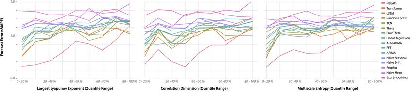
Figure 1: Properties of the chaotic dynamical systems dataset. (A) Embeddings of 131 chaotic
dynamical systems. Points correspond to average embeddings of individual systems, and shading
shows ranges over many random initial conditions. Colors correspond to an unsupervised clustering,
and example dynamics for each cluster are shown. (B) Distributions of key mathematical properties
across the dataset.
modelling: (1) Chaotic systems have provably complex dynamics, which arise due to underlying
mathematical structure, rather than complex representation of otherwise simple latent dynamics. (2)
Existing time series databases contain datasets chosen primarily for availability or applicability, rather
than for having innate properties (e.g. complexity, quasiperiodicity, dimensionality) that span the
range of possible behaviors time series may exhibit. (3) Chaotic systems have accessible generating
processes, making it possible to obtain new data and representations, and for the benchmark to
be related to mechanistic details of the underlying system. These properties suggest that chaotic
systems can aid in interpreting the properties of complex models [6, 106]. However, chaotic systems
as benchmarks lack standardization, and prior works’ emphasis on single systems like the Lorenz
attractor may undermine generalizability. Moreover, focusing on isolated systems neglects the
diversity of dynamics in known chaotic systems, thereby preventing systematic quantification and
interpretation of algorithm performance relative to the mathematical properties of different systems.
Here, we present a growing database of low-dimensional chaotic systems drawn from published
work in diverse domains such as meteorology, neuroscience, hydrodynamics, and astrophysics. Each
system is represented by several multivariate time series drawn from the dynamics, annotations of
known mathematical properties, and an explicit analytical form that can be re-integrated to generate
new time series of arbitrary length, stochasticity, and granularity. We provide extensive forecasting
benchmarks across our systems, allowing us to interpret the empirical performance of different
forecasting techniques in the context of mathematical properties such as system chaoticity. Our
dataset improves the interpretability of time series algorithms by allowing methods to be compared
across time series with different intrinsic properties and underlying generating processes—thereby
complementing existing interpretability methods that identify salient feature sets or time windows
within single time series [22, 23]. We also consider applications to data-driven modelling in the form
of symbolic regression and neural ordinary differential equations tasks, and we show the surprising
result that the accuracy of a symbolic regression-derived formula can correlate with mathematical
properties of the dynamics produced by the formula. Finally, we demonstrate unique applications
enabled by the ability to re-integrate our dataset: we pre-train a timescale-matched feature extractor
for an existing time series classification benchmark, and we accelerate training of a forecast model by
importance sampling sparse regions on the dynamical attractor.

2   Description of Datasets

Scope. The diverse dynamical systems in our dataset span astrophysics, neuroscience, ecology,
climatology, hydrodynamics, and many other domains. The supplementary material contains a
glossary defining key terms from dynamical systems theory relevant to our dataset. Each entry in
our dataset represents a single dynamical system, such as the Lorenz attractor, that takes an initial

                                                    2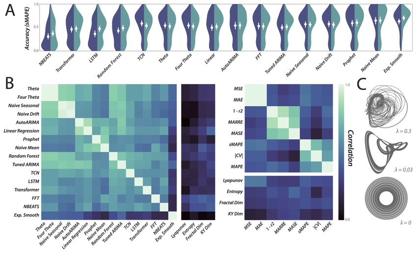
condition as input and outputs a trajectory representing the input point’s location as time evolves.
Systems are chosen based on prior appearance as named systems in published works. In order to
provide a consistent test for time series models, we define chaos in the mathematical sense: two
copies of a system prepared in infinitesimally different initial states will exponentially diverge over
time. We also focus particularly on chaotic systems that produce low-dimensional strange attractors,
which are fractal structures that display bounded, stationary, and ergodic dynamics with quantifiable
mathematical properties. As a result, we exclude transient chaos and chaotic repellers (chaotic
regions that trajectories eventually escape) [24–26], as well as most nonchaotic strange attractors
save for one paradigmatic example: a quasiperiodic two-dimensional torus [27].

Scale and structure. Our extensible collection currently comprises 131 previously-published and
named chaotic dynamical systems. Each record includes a compilable implementation of the system,
a citation reference, default initial conditions on the attractor, precomputed train and test trajectories
from different initial conditions at both coarse and fine granularities, and an optimal integration
timestep and dominant timescale (used for aligning timescales across systems). For each of the 131
systems, we include 16 precomputed trajectories corresponding to all combinations of the following
variations per system: coarse and fine sampling granularity, train and test splits emanating from
different initial conditions, multivariate and univariate views, and trajectories with and without
Brownian noise influencing the dynamics. Because certain data-driven modelling methods, such as
our symbolic regression task below, require gradient information, we also include with each system
precomputed train and test regression datasets corresponding to trajectories and time derivatives
along them.
Figure S1 shows the attractors for all systems, and Table S1 includes brief summaries of their origin
and applications. While there are an infinite number of possible chaotic dynamical systems, our work
represents, to our knowledge, the first effort to survey and reproduce previously-published chaotic
systems. For this reason, while our dataset is readily extensible to new systems, the primary bottleneck
as we expand our database is the need to manually reproduce claimed chaotic dynamics, and to
identify appropriate parameter values and initial conditions based on published reports. Broadly,
our work can be considered a systematization of previous studies that benchmark methods on single
chaotic systems such as the Lorenz attractor [9–11, 13–20, 126].

Annotations. For each system, we calculate and include precise estimates of several standard
mathematical characteristics of chaotic systems. More detailed definitions are included in the
appendix.
The largest Lyapunov exponent measures the degree to which nearby trajectories diverge, a common
measure of the degree of chaos present in a system.
The Lyapunov exponent spectrum determines the tendency of trajectories to locally converge or
diverge across the attractor. All continuous-time chaotic systems have at least one positive exponent,
exactly one zero exponent (due to time translation), and, for dissipative systems (i.e., those converging
to an attractor), at least one negative exponent [28].
The correlation dimension measures an attractor’s effective fractal dimension, which informally
indicates the intricacy of its geometric structure [4, 29]. Integer fractal dimensions indicate familiar
geometric forms: a line has dimension one, a plane has two, and a filled solid three. Non-integer
values correspond to fractals that fill space in a manner intermediate to the two nearest integers.
The multiscale entropy represents the degree to which complex dynamics persist across timescales
[111]. Chaotic systems have continuous power spectra, and thus high multiscale entropy.
We also include two quantities derived from the Lyapunov spectrum: the Pesin entropy bound, and the
Kaplan-Yorke fractal dimension, an alternative estimator of attractor dimension based on trajectory
dispersion. Each system is also annotated with various qualitative details, such as whether the system
is Hamiltonian or dissipative (i.e., whether there exists conserved invariants like total energy, or
whether the dynamics relax to an attractor), non-autonomous (whether the dynamical equations
explicitly depend on time), bounded (all variables remain finite as time passes), and whether the
dynamics are given by a delay differential equation. In addition to the 131 differential equations
described here, our collection also includes several common discrete time maps; however, we exclude
these from our study due to their unique properties.

                                                    3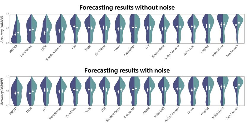
Methods. Our dataset includes utilities for re-sampling and re-integrating each system with or
without stochasticity, loading pre-computed multivariate or univariate trajectories, computing sta-
tistical properties and performing surrogate significance testing, and running benchmarks. One
shortcoming of previous studies using chaotic systems as benchmarks—as well as more generally
with static time series databases—is inconsistent timescales and granularities (sampling rates). We
alleviate this problem by using phase surrogate significance testing to select optimal integration
timesteps and sampling rates for all systems in our dataset, thus ensuring that dynamics are aligned
across systems with respect to dominant and minimum significant timescales [106]. We further
ensure consistency across systems using several standard methods, such as testing ergodicity to find
consistent initial conditions, and integrating with continuous re-orthonormalization when computing
various mathematical quantities such as Lyapunov exponents (see supplementary material).

Properties and Characterization. In order to characterize the properties of our collection, we use
an off-the-shelf time series featurizer that computes a corpus of 787 common time series features (e.g.
absolute change, peak count, wavelet transform coefficients, etc) for each system in our dataset [113].
In addition to providing general statistical descriptors for our systems, embedding and clustering the
systems based on these features illustrates the diverse dynamics present across our dataset (Figure
1). We find that the dynamical systems naturally separate into groups displaying different types of
chaotic dynamics, such as smooth scroll-like trajectories versus spiking. Additionally, we observe
that our chaotic systems trace a filamentary manifold in embedding space, a property consistent with
the established rarity of chaotic attractors within the space of possible dynamical systems: persistent
chaos often occurs in an intermediate regime between bifurcations producing simpler dynamics, such
as limit cycles or quiescence at fixed points [26, 105].

2.1   Prior Work.

Data-driven modelling and control. Many techniques at the intersection of machine learning and
dynamical systems theory have been evaluated on specific well-known chaotic attractors, such as
the Lorenz, Rössler, double pendulum, and Chua systems [9–11, 13–20, 126]. These and several
other chaotic systems used in previous machine learning studies are all included within our dataset
[109, 136].
General databases of analytical mathematical models include the BioModels database of systems
biology models, which currently contains 1017 curated entries, with an additional 1271 unreviewed
user submissions [34]. Among these models, a subset corresponding to 491 differential equations
recur within the ODEBase database [35]. For the specific task of symbolic regression, the inference
of analytical equations from data, existing benchmarks include the Nguyen dataset of 12 complex
mathematical expressions [36], and corpora of equations from two physics textbooks [37, 38, 104],
and a recently-released suite of 252 regression problems from Penn Machine Learning Benchmark
[129].

Forecasting and classification of time series. The UCR-UEA time series classification benchmark
includes 128 univariate and 30 multivariate time series with ~101 –103 timepoints [42, 44, 123, 128].
Several of these entries overlap with the UCI Machine Learning Repository, which contains 121
time series (91 multivariate) of lengths ~101 –106 [45]. The M-series of time series forecasting
competitions have most recently featured 106 univariate time series of length ~101 –105 [46]. The
recently-introduced Monash forecasting archive comprises 26 domain areas, each of which includes
~101 –106 distinct time series with lengths in the range ~102 –106 timepoints [121]. A recent long-
sequence forecasting model uses the ETT-small dataset of electricity consumption in two regions of
China (70,080 datapoints at one-minute increments) [48], as well as NOAA local climatological data
(~106 hourly recordings from ~103 locations) [49]. The PhysioNet database contains several hundred
physiological recordings such as EEG, ECG, and blood pressure, at a wide variety of resolutions and
lengths [50].
A point of differentiation between our work and existing datasets is our focus on reproducible chaotic
dynamics, which sufficiently narrows the space of potential systems that we can manually curate and
re-implement reported dynamics, and calculate key mathematical properties relevant to forecasting
and physics-based model inference. These mathematical properties can be used to interpret the
properties of black box models by examining their correlation with model performance across
systems. Our dataset’s curation also ensures a high degree of standardization across systems, such as

                                                  4
Figure 2: Forecasting benchmarks for all chaotic dynamical systems. (A) Distribution of forecast
errors for all dynamical systems and for all forecasting models, sorted by increasing median error.
Dark and light hues correspond to coarse and fine time series granularities. (B) Spearman correlation
among forecasting models, among different forecast evaluation metrics, and between forecasting
metrics and underlying mathematical properties, computed across all dynamical systems at fine
granularity. Columns are ordered by descending maximum cross-correlation in order to group similar
models and metrics. (C) The systems with the highest, median, and lowest forecasting error across
all models, annotated by largest Lyapunov exponent.
consistent integration and sampling timescales, as well as ergodicity and stationarity. Additionally,
the precomputed multivariate time series in our dataset approximately match the length and size
of existing time series databases. We emphasize that, unlike existing time series databases, our
dataset’s size is flexible due to the ability to re-integrate each system at arbitrary length, sample at
any granularity, integrate from new initial conditions, change the amount of stochastic forcing, or
even perturb parameters in the underlying differential equation in order to modify or control each
system’s dynamics.
3 Experiments
Task 1: Forecasting
Chaotic systems are inherently unpredictable, and extensive work by the physics community has
sought to quantify chaos, and to relate its properties to general features of the underlying governing
equations [6, 105]. Traditionally, the predictability of a chaotic system is thought to be determined by
the largest Lyapunov exponent, which measures the rate at which trajectories emanating from two
infinitesimally-spaced points will exponentially separate over time [28].
We evaluate this claim on our dataset by benchmarking 16 forecasting models spanning a wide variety
of techniques: deep learning methods (NBEATS, Transformer, LSTM, and Temporal Convolutional
Network), statistical methods (Prophet, Exponential Smoothing, Theta, 4Theta), common machine
learning techniques (Random Forest), classical methods (ARIMA, AutoARIMA, Fourier transform
regression), and standard naive baselines (naive mean, naive seasonal, naive drift) [117, 119–121].
Our train and test datasets correspond to differential initial conditions, and we perform separate
hyperparameter tuning for each chaotic system and granularity [117, 118]. While the forecasting
models are heterogenous, for each we tune whichever hyperparameter most closely corresponds to
a timescale—for example, the lag order for autoregressive models, or the input chunk size for the
5neural network models. Because all systems are aligned to the same average period, the range of
values over which timescales are tuned is scaled by the granularity. Hyperparameters are tuned using
held-out future values, and scores are computed on an unseen test trajectory emanating from different
initial conditions.
Our results are shown in Figure 2 for all dynamical systems at coarse and fine sampling granularity.
We include corresponding results for systems with noise in the supplementary material. We find
the the deep learning models perform particularly well, with the Transformer and NBEATS models
achieving the lowest median scores, while also appearing within the three best-performing models
for nearly all systems. On many datasets, the temporal convolutional network and traditional LSTM
models also achieve competitive performance. Notably, the random forest also exhibits strong
performance despite the continuous nature of our datasets, and with substantially lower training
cost. The relative ranking of the different forecasting models remains stable both as granularity is
varied over two orders of magnitude, and as noise is increased to a level dominating the signal (see
supplementary experiments). In the latter case, we observe that the performance of different models
converges as their overall performance decreases. Overall, NBEATS strongly outperforms the other
forecasting techniques across varied systems and granularities, and its performance persists even in
the presence of noise. We speculate that NBEAT’s advantage arises from its implicit decomposition
of time series into a hierarchy of basis functions [119], an approach that mirrors classical techniques
for representing continuous-time chaotic systems [55].
Our results seemingly contrast with studies showing that statistical models outperform neural net-
works on forecasting tasks [46, 121]. However, our forecasting task focuses on long time series
and prediction horizons, two areas where neural networks have previously performed well [48].
Additionally, we hypothesize that the strong performance of deep learning models on our dataset
is a consequence of the smoothness of chaotic systems, which have mathematical regularity and
stationarity compared to time series generated from industrial or environmental measurements. In
contrast, models like Prophet are often applied to calendar data with seasonality and irregularities
like holidays [56]—neither of which have a direct analogue in chaotic systems, which contain a
continuous spectrum of frequencies [57]. Consistent with this intuition, we observe that among the
systems in our dataset, the Prophet model performs well on the torus, a quasiperiodic system with
largest Lyapunov exponent equal to zero.
Several recent works have considered the appropriate metric for determining forecast accuracy
[46, 58, 59, 121]. For all forecasting models and dynamical systems we compute eight error metrics:
the mean squared error (MSE), mean absolute scaled error (MASE), mean absolute error (MAE),
mean absolute ranged relative error (MARRE), the magnitude of the coefficient of variation (|CV |),
one minus the coefficient of determination (1 − r2 ), and the symmetric and regular mean absolute
percent errors (MAPE and sMAPE). We find that all of these potential metrics are positively correlated
across our dataset, and that they can be grouped into families of strongly-related metrics (Figure
2B). We also observe that the relative ranking of different forecasting models is independent of the
choice of metric. Hereafter, we report sMAPE errors when comparing models, but we include all
other metrics within the benchmark.
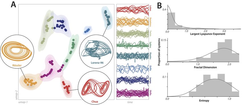
We next evaluate the common claim that the empirical predictability of a system depends on the
mathematical degree of chaos present [7]. For each system, we correlate the forecast error of the
best-performing model with the various mathematical properties of each system (Figure 2B). Across
all systems, we find a high degree of correlation between the largest Lyapunov exponent and the
forecast error, while other measures such as the attractor fractal dimension and entropy correlate less
strongly. While this observation matches conventional wisdom, it represents (to our knowledge) the
first large-scale test of the empirical relevance of Lyapunov exponents. We consider this observation
particularly noteworthy because our forecasting task spans several periods, yet the Lyapunov exponent
is a purely local measure of dispersion between infinitesimally-separated points.
Our results introduce several considerations for the development of time series models. The strong
performance we observe for neural network models implies that the flexibility of large models proves
beneficial for time series without obvious trends or seasonality. The consistent accuracy we observe
for NBEATS, even in the presence of noise, suggests that hierarchical decomposition can improve
modelling of systems with multiple timescales. Most of our best-performing methods implicitly
lift the dimensionality of the input time series, implying that higher-dimensional representations
create more predictable dynamics—a finding consistent with recent studies showing that certain
6Table 1: (Upper) Forecast accuracy for LSTMs trained on full time series, random subsets, and subsets
sampled proportionately to their epochwise error (medians ± standard errors across all dynamical
systems). (Lower) Accuracy scores on the UCR database for classifiers trained on features extracted
from bare time series, and from autoencoders pretrained on the full chaotic systems collection at
random and task-matched timescales (medians ± standard errors across UCR tasks).
Importance Sampling Forecasting Error (sMAPE)
Full Epochs Random Subset Importance Weighted
sMAPE 1.00 ± 0.05 0.99 ± 0.05 0.90 ± 0.05
Runtime (sec) 190.1 ± 0.3 77.9 ± 0.3 94.6 ± 0.2
Transfer Learning Classification Accuracy
No Transfer Learning Random Timescales Matched Surrogates
sMAPE 0.80 ± 0.02 0.82 ± 0.01 0.84 ± 0.01
machine learning techniques implicitly learn Koopman operators, linear propagators that act on
lifted representations of nonlinear systems [10, 57, 60–62]. That higher dimensional representations
can linearize dynamics mirrors classical motivation for kernel methods in machine learning [122];
we thus hypothesize that classical time series representations like time-lagged embeddings can be
improved through nonlinearities, either in the form of custom functions learned by neural networks,
or by inductive biases in the form of fixed periodic or wavelet-like kernels.
Task 2: Accelerating model training with importance sampling.
When training a forecasting model iteratively, each training batch usually samples input timepoints
with equal probability. However, chaotic attractors generally possess non-uniform measure due to
their fractal structure [64]. We thus hypothesize that importance sampling can accelerate training
of a forecast model, by encouraging the network to oversample sparser regions of the underlying
attractor [65]. We thus modify the training procedure for a forecast model by applying a simple form
of importance sampling, based on the epoch-wise training losses of individual samples—an approach
related to zeroth-order adaptive methods appearing in other areas [66–69]. Our procedure consists
of the following: (1) We halt training every few epochs and compute historical forecasts (backtests)
on the training trajectory. (2) We randomly sample timepoints proportionately to their error in the
historical forecast, and then generate a set of initial conditions corresponding to random perturbations
away from each sampled attractor point. (3) We simulate the full dynamical system for τ timesteps
for each of these initial conditions, and we use these new trajectories as the training set for the next b
epochs. We repeat this procedure for ν meta-epochs. For the original training procedure, the training
time scales as ∼ B, the number of training epochs. In our modified procedure, the training time has
dominant term ∼ ν b, plus an additional term proportional to τ (integration can be parallelized across
initial conditions), plus a small constant cost for sampling. We thus set ν b < B, and record run times
to verify that total cost has decreased.
Table 1 shows the results of our experiments for an LSTM model across all chaotic attractors.
Importance sampling achieves a significantly smaller forecast error than a baseline using the full
training set in each epoch, as well as a control in which the exact importance sampling procedure
was repeated without weighting random samples by error (two sided paired t-test, p < 10−6 for both
tests). Notably, importance sampling requires substantially lower computation due to the reduced
number of training epochs incurred. Our approach exploits that our database comprises strange
attractors, because initial conditions derived from random perturbations off an attractor will produce
trajectories that return to the attractor.
Task 3: Transfer learning and data augmentation.
We next explore how our dataset can assist general time series analysis, regardless of the relevance
of chaos to the problem. We study an existing time series classification benchmark, and we use our
dataset to generate timescale-matched surrogate data for transfer learning.
7Our classification procedure broadly consists of training an autoencoder on trajectories from our
database, and then using the trained encoder as a general feature extractor for time series classification.
However, unlike existing transfer learning approaches for time series [70], we train the autoencoder
on a new dataset for each classification problem: we re-integrate our entire dataset to match the
dominant timescales in the classification problem’s training data.
Our approach thus comprises several steps: (1) Across all data in the train partition, the dominant
significant Fourier frequency is determined using random phase surrogates [106]. (2) Trajectories
are re-integrated for every dynamical system in our database, such that the sampling rate of the
dynamics is equal to that of the training dataset. The surrogate ensemble thus corresponds to a
custom set of trajectories with timescales matched to the training data of the classification problem.
(3) We train an autoencoder on this ensemble. Our encoder is a one layer causal dilated encoder
with skip connections, an architecture recently shown to provide strong time series classification
performance [124]. (3) We apply the encoder to the training data of the classification problem. (4)
We apply a standard linear time series classifier, following recent works [116, 128]. We featurize the
time series using a library of standard featurizers [113], and then perform classification using ridge
regression [116]. Overall, our classification approach bears conceptual similarity to other generative
data augmentation techniques: we extract parameters (the dominant timescales) from the training data,
and then use these parameters to construct a custom surrogate ensemble with matching timescales. In
many image augmentation approaches, a prior distribution is learned from the training data (e.g. via a
GAN), and the then sampled to create surrogate examples [73–76].
As baselines for our approach, we train a classifier on the
0.56
bare original time series, as well as a "random timescale"
Final Accuracy
collection in which the time series in the surrogate ensem-
ble have random dominant frequencies, unrelated to the
timescales in the training data. The latter ablation serves
to isolate the role of timescale matching, which is uniquely
enabled by the ability to re-integrate our dataset at arbi-
trary granularity. This is necessary in light of recent work
showing that transfer learning on a large collection of time 0.46
series can yield informative features [70].
0.0 1.0
We benchmark classification using the UCR time se- Fraction of Dataset
ries classification benchmark, which contains 128 real-
Figure 3: Classification accuracy on the
world classification problems spanning diverse areas like
UCR dataset EOGHorizontalSignal,
medicine, agriculture, and robotics [123]. Because we are
across models pretrained on increasing
using convolutional models, we restrict our analysis to the
fractions of the database. Standard errors
91 datasets with at least 100 contiguous timepoints (these
are from bootstrapped replicates, where
include the 85 "bakeoff" datasets benchmarked in previous
the dynamical systems are sampled with
studies) [42]. We compute separate benchmarks (surrogate
replacement.
ensembles, features, and scores) for each dataset in the
archive.
Our results are shown in Table 1. Across the UCR archive we observe statistically significant average
classification accuracy increases of 4% ± 1% compared to the raw dataset (p < 10−4 , paired two-
sided t-test), and 2% ± 1% compared to the ablation with random surrogate timescales (p < 10−4 ).
While these modest improvements do not comprise state-of-the-art results on the UCR database
[42], they demonstrate that features learned from chaotic systems in an unsupervised setting can
be used to extract meaningful general features for further analysis. On certain datasets, our results
approach other recent unsupervised approaches in which a simple linear classifier is trained on top
of a complex unsupervised feature extractor [70, 124, 128]. Recent results have even shown that a
very large number of random convolutional features can provide informative representations of time
series for downstream supervised learning tasks [128]; we therefore speculate that pretraining with
chaotic systems may allow more efficient selection of informative convolutional kernels. Moreover,
the improvement of transfer learning over the random timescale model demonstrates the advantage of
re-integration. In order to verify that the diversity of dynamical systems present within our dataset
contribute to the quality of the learned features, we repeat the classification task on a single UCR
dataset, corresponding to clinical eye tracking data. We train encoders on gradually increasing
numbers of dynamical systems, in order to see how the final accuracy changes as the number of
8A 3.0 B 0.2
Lyapunov
Error (sMAPE)
Correlation
2.0 Entropy
0.0
Fractal Dim
1.0
KY Dim
0.0 -0.2
r
ly
r
R
R
y
R
R
ie
ie
ol
DS
DS
S
S
po
py
py
ur
ur
p
Y-
Y-
fo
fo
ND
ND
Y-
Y-
ND
ND
SI
SI
SI
SI
Figure 4: Symbolic regression benchmarks. (A) Error distributions on test datasets across all
systems, (B) Spearman correlation between errors and mathematical properties of the underlying
systems.
systems available for pretraining increases (Figure 3). We observe monotonic scaling, indicating that
our dataset’s size and diversity contribute to feature quality.
Task 4: Data-driven model inference and symbolic regression
We next look beyond traditional time series analysis, and apply our database to a data-driven
modelling task. A growing body of work uses machine learning methods to infer dynamical systems
directly from data [77–80]. Examples include constructing effective propagators for the dynamics
[57, 61, 62, 81–83], obtaining neural representations of the dynamical equations [85–87, 131], and
inferring analytical governing equations via symbolic regression [37, 60, 89–93, 129, 130]. Beyond
improving forecasts, these data-driven representations can discover mechanistic insights, such as
symmetries or separated timescales, that might not otherwise be apparent in a time series.
We thus use our dataset for data-driven modelling in the form of a symbolic regression task. We
focus on symbolic regression because of the recent emergence of widely-used benchmark models
and performance desiderata for these methods [129]. However, we emphasize that our database
can be used for other emerging focus areas in data-driven modelling, such as inference of empirical
propagators or neural ordinary differential equations [57, 82, 94], and we include a baseline neural
ordinary differential equation task in the supplementary material. For each dynamical system in
our collection, we generate trajectories with sufficiently coarse granularity to sample all regions of
the attractor. At each timepoint, we compute the value of the right hand side of the corresponding
dynamical equation, and we treat the value of this time derivative as the regression target. We use
this dataset to compare several recent symbolic regression approaches: (1) DSR: a recurrent neural
network trained with a risk-seeking policy gradient, which produces state-of-the-art results on a
variety of challenging symbolic regression tasks [130]. (2) PySR: an open-source package inspired by
the popular closed-source software Eureqa, which uses genetic programming and simulated annealing
[90, 92, 95]. (3,4) PySINDY: a Python implementation of the widely-used SINDY algorithm, which
uses sparse regression to decompose data into linear combinations of functions [89, 96]. For PySINDY
we train separate models for purely polynomial (SINDY-poly) and trigonometric (SINDY-fourier)
bases. For DSR and pySR we use a standard library of binary and unary expressions, {+, −, ×, ∇·},
{sin, cos, exp, log, tanh} [130]. After fitting a formula using each method, we evaluate it on an
unseen test trajectory arising from different initial conditions, and we report the the sMAPE error
between the formula’s prediction and the true value along the trajectory.
Our results illustrate several features of our dataset, while also illustrating properties of the different
symbolic regression algorithms. All algorithms show strong performance across the chaotic systems
dataset (Figure 4). The two lowest-error models, pySR and DSR, exhibit nearly-equivalent perfor-
mance when accounting for error ranges, and both achieve errors near zero on many systems. We
attribute this strong performance to the relatively simple algebraic construction of most published
systems: named chaotic systems will inevitably favor concise, demonstrative equations over complex
expressions. In fact, several systems in our dataset belong to the Sprott attractor family, which
represent the algebraically simplest chaotic systems [97]. In this sense, our dataset likely has similar
complexity to the Feynman equations benchmark [37].
We highlight that PySINDY with a purely polynomial basis performs very well on our dataset,
especially as a linear approach that requires a median training time of only 0.01 ± 0.01 s per system
on a single CPU core. In comparison, pySR had a median time of 1400 ± 60 s per system on one
9core, while DSR on one GPU required 4300 ± 200s per system—consistent with the results of recent
symbolic regression benchmark suite [129]. However, parallelization reduces the runtime of all
methods.
We emphasize that the relative performance of a given symbolic regression algorithm depends on
diverse factors, such as equation complexity, the library of available unary and binary operators, the
amount and dynamic range of available input data, the amount of compute available for refinement,
and the degree of nonlinearity of the underlying system. More generally, symbolic regression algo-
rithms exhibit a bias-variance tradeoff manifesting as Pareto front bridging accuracy and parsimony:
large models with many terms will appear more accurate, but at the expense of brevity and potentially
robustness and interpretability [90]. More challenging benchmarks would include nested expressions
and uncommon transcendental functions; these systems may be a more appropriate setting for bench-
marking state-of-the-art techniques like DSR. Additionally, we do not include measurement noise in
our experiments, a scenario in which DSR performs strongly compared to other methods [129, 130].
Interestingly, DSR exhibits the strongest dependence on the mathematical properties of the underlying
dynamics: more chaotic systems consistently yield higher errors (Figure 4B). We consider this
result surprising, because a priori we would expect the performance of a given symbolic regression
algorithm to depend purely on the syntactic complexity of the target formula, rather than the dynamics
that it produces. Because DSR uses a large model to navigate a space of smaller models, we
hypothesize that more chaotic systems present a broader set of possible "partial formulae" that match
specific subregimes of the attractor—an effect exploited in several recent decomposition techniques
for chaotic systems [9, 11]. The diversity of these local approximants would result in a more complex
global search space.
4 Discussion
We have introduced an extensible collection of known chaotic dynamical systems. In addition to
representing a customizable benchmark for time series analysis and data-driven modelling, we have
provided examples of additional applications, such as transfer learning for general time series analysis
tasks, that are enabled by the generative nature of our dataset. We note that there are several other
potential applications that we have not explored here: testing feedback-based control algorithms
(which require perturbing the parameters of a given dynamical system, and then re-integrating),
and inferring numerical propagators (such as Koopman operators)[57, 61, 62, 81–83, 98, 99]. In
the appendix, we include preliminary benchmarks for a neural ordinary differential equations task
[85–87, 131]; due to the direct connections between our work and this area, we hope to further explore
these methods in future studies. Our work can be seen as systematizing the common practice of
testing new methods on single chaotic systems, particularly the Lorenz attractor [9–11, 13–20, 126].
More broadly, our collection seeks to improve the interpretability of data-driven modelling from time
series. For example, our forecasting benchmark experiments show that the Lyapunov exponent, a
popular measure of local chaoticity, correlates with the empirical predictability of a system under a
variety of models—a finding that matches intuition, but which has not (to our knowledge) previously
been tested extensively. Likewise, in our symbolic regression benchmark we find that more chaotic
systems are harder to model, an effect we attribute to the diverse local approximants available for
complex dynamical systems. These examples demonstrate how the control and mathematical context
provided by differential equations can yield mechanistic insight beyond traditional time series.
Limitations of our approach include our inclusion only of known chaotic systems that have previously
appeared in published works. This limits the rate at which our collection may expand, since each new
entry requires manual curation and implementation in order to verify reported dynamics. Our focus
on published systems may bias the dataset towards more unusual (and thus reportable) dynamics,
particularly because there are infinite possible chaotic systems. Moreover, in few dimensions
chaotic dynamics are rare relative to the space of all possible models [105], although chaos becomes
ubiquitous as the number of coupled variables increases [100]. Nonetheless, low-dimensional chaos
may represent an instructive step towards understanding complex dynamics in high-dimensional
systems.
10Acknowledgments and Disclosure of Funding
We thank Gautam Reddy, Samantha Petti, Brian Matejek, and Yasa Baig for helpful discussions and
comments on the manuscript. W. G. was supported by the NSF-Simons Center for Mathematical and
Statistical Analysis of Biology at Harvard University, NSF Grant DMS 1764269, and the Harvard
FAS Quantitative Biology Initiative. The author declares no competing interests.
References
[1] Crutchfield, J. & Packard, N. Symbolic dynamics of one-dimensional maps: Entropies, finite
precision, and noise. International Journal of Theoretical Physics 21, 433–466 (1982).
[2] Cvitanovic, P. et al. Chaos: classical and quantum, vol. 69 (Niels Bohr Institute, Copenhagen,
2005). URL http://chaosbook.org/.
[3] Farmer, J. D. Information dimension and the probabilistic structure of chaos. Zeitschrift für
Naturforschung A 37, 1304–1326 (1982).
[4] Grebogi, C., Ott, E. & Yorke, J. A. Chaos, strange attractors, and fractal basin boundaries in
nonlinear dynamics. Science 238, 632–638 (1987).
[5] Ott, E. Chaos in Dynamical Systems (Cambridge University Press, 2002).
[6] Tang, Y., Kurths, J., Lin, W., Ott, E. & Kocarev, L. Introduction to focus issue: When machine
learning meets complex systems: Networks, chaos, and nonlinear dynamics. Chaos: An
Interdisciplinary Journal of Nonlinear Science 30, 063151 (2020).
[7] Pathak, J., Hunt, B., Girvan, M., Lu, Z. & Ott, E. Model-free prediction of large spatiotempo-
rally chaotic systems from data: A reservoir computing approach. Physical review letters 120,
024102 (2018).
[8] Boffetta, G., Cencini, M., Falcioni, M. & Vulpiani, A. Predictability: a way to characterize
complexity. Physics reports 356, 367–474 (2002).
[9] Nassar, J., Linderman, S., Bugallo, M. & Park, I. M. Tree-structured recurrent switching
linear dynamical systems for multi-scale modeling. In International Conference on Learning
Representations (2018).
[10] Champion, K., Lusch, B., Kutz, J. N. & Brunton, S. L. Data-driven discovery of coordinates
and governing equations. Proceedings of the National Academy of Sciences 116, 22445–22451
(2019).
[11] Costa, A. C., Ahamed, T. & Stephens, G. J. Adaptive, locally linear models of complex
dynamics. Proceedings of the National Academy of Sciences 116, 1501–1510 (2019).
[12] Gilpin, W. Deep reconstruction of strange attractors from time series. Advances in Neural
Information Processing Systems 33 (2020).
[13] Greydanus, S. J., Dzumba, M. & Yosinski, J. Hamiltonian neural networks. In Advances in
Neural Information Processing Systems, 2794–2803 (2019).
[14] Lu, Z., Kim, J. Z. & Bassett, D. S. Supervised chaotic source separation by a tank of water.
Chaos: An Interdisciplinary Journal of Nonlinear Science 30, 021101 (2020).
[15] Yu, R., Zheng, S., Anandkumar, A. & Yue, Y. Long-term forecasting using tensor-train rnns.
arXiv preprint arXiv:1711.00073 (2017).
[16] Lu, Z. et al. Reservoir observers: Model-free inference of unmeasured variables in chaotic
systems. Chaos: An Interdisciplinary Journal of Nonlinear Science 27, 041102 (2017).
[17] Bellot, A., Branson, K. & van der Schaar, M. Consistency of mechanistic causal discovery in
continuous-time using neural odes. arXiv preprint arXiv:2105.02522 (2021).
11[18] Wang, Z. & Guet, C. Reconstructing a dynamical system and forecasting time series by
self-consistent deep learning. arXiv preprint arXiv:2108.01862 (2021).
[19] Li, X., Wong, T.-K. L., Chen, R. T. & Duvenaud, D. Scalable gradients for stochastic
differential equations. In International Conference on Artificial Intelligence and Statistics,
3870–3882 (PMLR, 2020).
[20] Ma, Q.-L., Zheng, Q.-L., Peng, H., Zhong, T.-W. & Xu, L.-Q. Chaotic time series prediction
based on evolving recurrent neural networks. In 2007 international conference on machine
learning and cybernetics, vol. 6, 3496–3500 (IEEE, 2007).
[21] Kantz, H. & Schreiber, T. Nonlinear time series analysis, vol. 7 (Cambridge university press,
2004).
[22] Ismail, A., Gunady, M., Bravo, H. & Feizi, S. Benchmarking deep learning interpretability
in time series predictions. Advances in Neural Information Processing Systems Foundation
(NeurIPS) (2020).
[23] Lim, B., Arık, S. Ö., Loeff, N. & Pfister, T. Temporal fusion transformers for interpretable
multi-horizon time series forecasting. International Journal of Forecasting (2021).
[24] Tél, T. The joy of transient chaos. Chaos: An Interdisciplinary Journal of Nonlinear Science
25, 097619 (2015).
[25] Chen, X., Nishikawa, T. & Motter, A. E. Slim fractals: The geometry of doubly transient
chaos. Physical Review X 7, 021040 (2017).
[26] Grebogi, C., Ott, E. & Yorke, J. A. Critical exponent of chaotic transients in nonlinear
dynamical systems. Physical review letters 57, 1284 (1986).
[27] Grebogi, C., Ott, E., Pelikan, S. & Yorke, J. A. Strange attractors that are not chaotic. Physica
D: Nonlinear Phenomena 13, 261–268 (1984).
[28] Sommerer, J. C. & Ott, E. Particles floating on a moving fluid: A dynamically comprehensible
physical fractal. Science 259, 335–339 (1993).
[29] Grassberger, P. & Procaccia, I. Measuring the strangeness of strange attractors. Physica D:
Nonlinear Phenomena 9, 189–208 (1983).
[30] Costa, M., Goldberger, A. L. & Peng, C.-K. Multiscale entropy analysis of complex physiologic
time series. Physical review letters 89, 068102 (2002).
[31] Christ, M., Braun, N., Neuffer, J. & Kempa-Liehr, A. W. Time series feature extraction on
basis of scalable hypothesis tests (tsfresh–a python package). Neurocomputing 307, 72–77
(2018).
[32] Myers, A. D., Yesilli, M., Tymochko, S., Khasawneh, F. & Munch, E. Teaspoon: A compre-
hensive python package for topological signal processing. In NeurIPS 2020 Workshop on
Topological Data Analysis and Beyond (2020).
[33] Datseris, G. DynamicalSystems.jl: A Julia software library for chaos and nonlinear dynamics.
Journal of Open Source Software 3, 598 (2018).
[34] Le Novere, N. et al. Biomodels database: a free, centralized database of curated, published,
quantitative kinetic models of biochemical and cellular systems. Nucleic acids research 34,
D689–D691 (2006).
[35] Lüders, C., Errami, H., Neidhardt, M., Samal, S. S. & Weber, A. Odebase: an extensible
database providing algebraic properties of dynamical systems. In Proceedings of the Computer
Algebra in Scientific Computing Conference (CASC, 2019).
[36] Uy, N. Q., Hoai, N. X., O’Neill, M., McKay, R. I. & Galván-López, E. Semantically-based
crossover in genetic programming: application to real-valued symbolic regression. Genetic
Programming and Evolvable Machines 12, 91–119 (2011).
12[37] Udrescu, S.-M. & Tegmark, M. Ai feynman: A physics-inspired method for symbolic
regression. Science Advances 6, eaay2631 (2020).
[38] La Cava, W., Danai, K. & Spector, L. Inference of compact nonlinear dynamic models by
epigenetic local search. Engineering Applications of Artificial Intelligence 55, 292–306 (2016).
[39] Strogatz, S. H. Nonlinear dynamics and chaos with student solutions manual: With applications
to physics, biology, chemistry, and engineering (CRC press, 2018).
[40] La Cava, W. et al. Contemporary symbolic regression methods and their relative performance.
arXiv preprint arXiv:2107.14351 (2021).
[41] Dau, H. A. et al. The ucr time series archive. IEEE/CAA Journal of Automatica Sinica 6,
1293–1305 (2019).
[42] Bagnall, A., Lines, J., Bostrom, A., Large, J. & Keogh, E. The great time series classification
bake off: a review and experimental evaluation of recent algorithmic advances. Data mining
and knowledge discovery 31, 606–660 (2017).
[43] Dempster, A., Petitjean, F. & Webb, G. I. Rocket: exceptionally fast and accurate time series
classification using random convolutional kernels. Data Mining and Knowledge Discovery 34,
1454–1495 (2020).
[44] Bagnall, A. et al. The uea multivariate time series classification archive, 2018. arXiv preprint
arXiv:1811.00075 (2018).
[45] Asuncion, A. & Newman, D. Uci machine learning repository (2007).
[46] Makridakis, S., Spiliotis, E. & Assimakopoulos, V. The m4 competition: 100,000 time series
and 61 forecasting methods. International Journal of Forecasting 36, 54–74 (2020).
[47] Godahewa, R., Bergmeir, C., Webb, G. I., Hyndman, R. J. & Montero-Manso, P. Monash time
series forecasting archive. arXiv preprint arXiv:2105.06643 (2021).
[48] Zhou, H. et al. Informer: Beyond efficient transformer for long sequence time-series forecast-
ing. In Proceedings of The Thirty-Fifth AAAI Conference on Artificial Intelligence, AAAI 2021,
vol. 35, 11106–11115 (AAAI Press, 2021).
[49] Young, A. H., Knapp, K. R., Inamdar, A., Hankins, W. & Rossow, W. B. The international
satellite cloud climatology project h-series climate data record product. Earth System Science
Data 10, 583–593 (2018).
[50] Goldberger, A. L. et al. Physiobank, physiotoolkit, and physionet: components of a new
research resource for complex physiologic signals. circulation 101, e215–e220 (2000).
[51] Oreshkin, B. N., Carpov, D., Chapados, N. & Bengio, Y. N-beats: Neural basis expansion
analysis for interpretable time series forecasting. arXiv preprint arXiv:1905.10437 (2019).
[52] Lea, C., Vidal, R., Reiter, A. & Hager, G. D. Temporal convolutional networks: A unified
approach to action segmentation. In European Conference on Computer Vision, 47–54
(Springer, 2016).
[53] Alexandrov, A. et al. GluonTS: Probabilistic and Neural Time Series Modeling in Python. J.
Mach. Learn. Res. 21, 1–6 (2020).
[54] Herzen, J. et al. Darts: User-friendly modern machine learning for time series. arXiv preprint
arXiv:2110.03224 (2021). URL https://arxiv.org/abs/2110.03224.
[55] Wang, W.-X., Yang, R., Lai, Y.-C., Kovanis, V. & Grebogi, C. Predicting catastrophes in
nonlinear dynamical systems by compressive sensing. Physical review letters 106, 154101
(2011).
[56] Taylor, S. J. & Letham, B. Forecasting at scale. The American Statistician 72, 37–45 (2018).
13[57] Lusch, B., Kutz, J. N. & Brunton, S. L. Deep learning for universal linear embeddings of
nonlinear dynamics. Nature communications 9, 1–10 (2018).
[58] Hyndman, R. J. & Koehler, A. B. Another look at measures of forecast accuracy. International
journal of forecasting 22, 679–688 (2006).
[59] Durbin, J. & Koopman, S. J. Time series analysis by state space methods (Oxford university
press, 2012).
[60] Klus, S. et al. Data-driven model reduction and transfer operator approximation. Journal of
Nonlinear Science 28, 985–1010 (2018).
[61] Otto, S. E. & Rowley, C. W. Koopman operators for estimation and control of dynamical
systems. Annual Review of Control, Robotics, and Autonomous Systems 4, 59–87 (2021).
[62] Takeishi, N., Kawahara, Y. & Yairi, T. Learning koopman invariant subspaces for dynamic
mode decomposition. arXiv preprint arXiv:1710.04340 (2017).
[63] Hastie, T., Tibshirani, R. & Friedman, J. The Elements of Statistical Learning: Data Mining,
Inference, and Prediction. Springer series in statistics (Springer, 2009). URL https://
books.google.com/books?id=eBSgoAEACAAJ.
[64] Farmer, J. D. Dimension, fractal measures, and chaotic dynamics. In Evolution of order and
chaos, 228–246 (Springer, 1982).
[65] Leitao, J. C., Lopes, J. V. P. & Altmann, E. G. Monte carlo sampling in fractal landscapes.
Physical review letters 110, 220601 (2013).
[66] Press, W. H., Flannery, B. P., Teukolsky, S. A. & Vetterling, W. Numerical recipices, the art of
scientific computing. Cambridge U. Press, Cambridge, MA (1986).
[67] Jiang, A. H. et al. Accelerating deep learning by focusing on the biggest losers. arXiv preprint
arXiv:1910.00762 (2019).
[68] Kawaguchi, K. & Lu, H. Ordered sgd: A new stochastic optimization framework for empirical
risk minimization. In International Conference on Artificial Intelligence and Statistics, 669–
679 (PMLR, 2020).
[69] Katharopoulos, A. & Fleuret, F. Not all samples are created equal: Deep learning with
importance sampling. In International conference on machine learning, 2525–2534 (PMLR,
2018).
[70] Malhotra, P., TV, V., Vig, L., Agarwal, P. & Shroff, G. Timenet: Pre-trained deep recurrent
neural network for time series classification. arXiv preprint arXiv:1706.08838 (2017).
[71] Franceschi, J.-Y., Dieuleveut, A. & Jaggi, M. Unsupervised scalable representation learning for
multivariate time series. Advances in Neural Information Processing Systems 32, 4650–4661
(2019).
[72] Löning, M. et al. sktime: A unified interface for machine learning with time series. arXiv
preprint arXiv:1909.07872 (2019).
[73] Zhang, X., Wang, Z., Liu, D. & Ling, Q. Dada: Deep adversarial data augmentation for
extremely low data regime classification. In ICASSP 2019-2019 IEEE International Conference
on Acoustics, Speech and Signal Processing (ICASSP), 2807–2811 (IEEE, 2019).
[74] Tran, T., Pham, T., Carneiro, G., Palmer, L. & Reid, I. A bayesian data augmentation approach
for learning deep models. In Advances in Neural Information Processing Systems, 2794–2803
(2017).
[75] Zhu, X., Liu, Y., Qin, Z. & Li, J. Data augmentation in emotion classification using generative
adversarial networks. arXiv preprint arXiv:1711.00648 (2017).
14[76] Hauberg, S., Freifeld, O., Larsen, A. B. L., Fisher, J. & Hansen, L. Dreaming more data: Class-
dependent distributions over diffeomorphisms for learned data augmentation. In Artificial
Intelligence and Statistics, 342–350 (PMLR, 2016).
[77] Karniadakis, G. E. et al. Physics-informed machine learning. Nature Reviews Physics 3,
422–440 (2021).
[78] de Silva, B. M., Higdon, D. M., Brunton, S. L. & Kutz, J. N. Discovery of physics from data:
universal laws and discrepancies. Frontiers in artificial intelligence 3, 25 (2020).
[79] Callaham, J. L., Koch, J. V., Brunton, B. W., Kutz, J. N. & Brunton, S. L. Learning dominant
physical processes with data-driven balance models. Nature communications 12, 1–10 (2021).
[80] Carleo, G. et al. Machine learning and the physical sciences. Reviews of Modern Physics 91,
045002 (2019).
[81] Costa, A. C., Ahamed, T., Jordan, D. & Stephens, G. Maximally predictive ensemble dynamics
from data. arXiv preprint arXiv:2105.12811 (2021).
[82] Budišić, M., Mohr, R. & Mezić, I. Applied koopmanism. Chaos: An Interdisciplinary Journal
of Nonlinear Science 22, 047510 (2012).
[83] Gilpin, W. Cellular automata as convolutional neural networks. Physical Review E 100,
032402 (2019).
[84] Chen, R. T., Rubanova, Y., Bettencourt, J. & Duvenaud, D. Neural ordinary differential
equations. arXiv preprint arXiv:1806.07366 (2018).
[85] Kidger, P., Morrill, J., Foster, J. & Lyons, T. Neural controlled differential equations for
irregular time series. arXiv preprint arXiv:2005.08926 (2020).
[86] Massaroli, S., Poli, M., Park, J., Yamashita, A. & Asama, H. Dissecting neural odes. arXiv
preprint arXiv:2002.08071 (2020).
[87] Rackauckas, C. et al. Universal differential equations for scientific machine learning. arXiv
preprint arXiv:2001.04385 (2020).
[88] Petersen, B. K. et al. Deep symbolic regression: Recovering mathematical expressions from
data via risk-seeking policy gradients. arXiv preprint arXiv:1912.04871 (2019).
[89] Brunton, S. L., Proctor, J. L. & Kutz, J. N. Discovering governing equations from data by
sparse identification of nonlinear dynamical systems. Proceedings of the national academy of
sciences 113, 3932–3937 (2016).
[90] Schmidt, M. & Lipson, H. Distilling free-form natural laws from experimental data. science
324, 81–85 (2009).
[91] Martin, B. T., Munch, S. B. & Hein, A. M. Reverse-engineering ecological theory from data.
Proceedings of the Royal Society B: Biological Sciences 285, 20180422 (2018).
[92] Cranmer, M. et al. Discovering symbolic models from deep learning with inductive biases.
NeurIPS 2020 (2020). 2006.11287.
[93] Rudy, S. H. & Sapsis, T. P. Sparse methods for automatic relevance determination. Physica D:
Nonlinear Phenomena 418, 132843 (2021).
[94] Froyland, G. & Padberg, K. Almost-invariant sets and invariant manifolds—connecting
probabilistic and geometric descriptions of coherent structures in flows. Physica D: Nonlinear
Phenomena 238, 1507–1523 (2009).
[95] Cranmer, M. Pysr: Fast & parallelized symbolic regression in python/julia (2020). URL
http://doi.org/10.5281/zenodo.4041459.
[96] de Silva, B. et al. Pysindy: A python package for the sparse identification of nonlinear
dynamical systems from data. Journal of Open Source Software 5, 1–4 (2020).
15You can also read