Ozone Monitoring Instrument (OMI) Aura nitrogen dioxide standard product version 4.0 with improved surface and cloud treatments
←
→
Page content transcription
If your browser does not render page correctly, please read the page content below
Atmos. Meas. Tech., 14, 455–479, 2021
https://doi.org/10.5194/amt-14-455-2021
© Author(s) 2021. This work is distributed under
the Creative Commons Attribution 4.0 License.

Ozone Monitoring Instrument (OMI) Aura nitrogen
dioxide standard product version 4.0 with improved
surface and cloud treatments
Lok N. Lamsal1,2 , Nickolay A. Krotkov2 , Alexander Vasilkov2,3 , Sergey Marchenko2,3 , Wenhan Qin2,3 ,
Eun-Su Yang2,3 , Zachary Fasnacht2,3 , Joanna Joiner2 , Sungyeon Choi2,3 , David Haffner2,3 , William H. Swartz4 ,
Bradford Fisher2,3 , and Eric Bucsela5
1 Goddard  Earth Sciences Technology & Research, Universities Space Research Association, Greenbelt, MD 20771, USA
2 Atmospheric  Chemistry and Dynamics Laboratory, NASA Goddard Space Flight Center, Greenbelt, MD 20771, USA
3 Science Systems and Applications, Lanham, MD 20706, USA
4 Applied Physics Laboratory, Johns Hopkins University, Laurel, MD 20723, USA
5 SRI International, Menlo Park, CA 94025, USA

Correspondence: Lok N. Lamsal (lok.lamsal@nasa.gov)

Received: 20 May 2020 – Discussion started: 29 June 2020
Revised: 9 November 2020 – Accepted: 24 November 2020 – Published: 21 January 2021

Abstract. We present a new and improved version (V4.0) of         face reflectance data sets. We quantitatively evaluate the new
the NASA standard nitrogen dioxide (NO2 ) product from the        NO2 product using independent observations from ground-
Ozone Monitoring Instrument (OMI) on the Aura satellite.          based and airborne instruments. The new V4.0 data and
This version incorporates the most salient improvements for       relevant explanatory documentation are publicly available
OMI NO2 products suggested by expert users and enhances           from the NASA Goddard Earth Sciences Data and Infor-
the NO2 data quality in several ways through improvements         mation Services Center (https://disc.gsfc.nasa.gov/datasets/
to the air mass factors (AMFs) used in the retrieval algo-        OMNO2_V003/summary/, last access: 8 November 2020),
rithm. The algorithm is based on the geometry-dependent           and we encourage their use over previous versions of OMI
surface Lambertian equivalent reflectivity (GLER) opera-          NO2 products.
tional product that is available on an OMI pixel basis. GLER
is calculated using the vector linearized discrete ordinate
radiative transfer (VLIDORT) model, which uses as input
high-resolution bidirectional reflectance distribution function   1   Introduction
(BRDF) information from NASA’s Aqua Moderate Resolu-
tion Imaging Spectroradiometer (MODIS) instruments over           The Dutch–Finnish-built Ozone Monitoring Instrument
land and the wind-dependent Cox–Munk wave-facet slope             (OMI) has been operating onboard the NASA EOS Aura
distribution over water, the latter with a contribution from      spacecraft since July 2004 (Levelt et al., 2006, 2018). The
the water-leaving radiance. The GLER combined with con-           primary objectives of OMI’s mission are to continue the
sistently retrieved oxygen dimer (O2 –O2 ) absorption-based       long-term record of total column ozone and to monitor other
effective cloud fraction (ECF) and optical centroid pres-         trace gases relevant to tropospheric pollution worldwide. Ob-
sure (OCP) provide improved information to the new NO2            servations of sunlight backscattered from the Earth over a
AMF calculations. The new AMFs increase the retrieved             wide range of UV and visible wavelengths (∼ 260–500 nm)
tropospheric NO2 by up to 50 % in highly polluted ar-             made by OMI allow for the retrieval of various atmospheric
eas; these differences arise from both cloud and surface          trace gases, including nitrogen dioxide (NO2 ). NO2 is a criti-
BRDF effects as well as biases between the new MODIS-             cally important short-lived air pollutant originating from both
based and previously used OMI-based climatological sur-           anthropogenic and natural sources. It is the principal precur-

Published by Copernicus Publications on behalf of the European Geosciences Union.
456                                            L. N. Lamsal et al.: OMI Aura nitrogen dioxide standard product version 4.0

sor to tropospheric ozone and a key agent for the formation of      partially mitigated by using a priori information from high-
several toxic airborne substances such as nitric acid (HNO3 ),      resolution CTM simulations (Russell et al., 2011; McLin-
nitrate aerosols, and peroxyacetyl nitrate. Satellite-based ob-     den et al., 2014; Lin et al., 2014, 2015; Goldberg et al.,
servations yield a global, self-consistent NO2 data record that     2017; Choi et al., 2020). Current global NO2 retrievals are
can complement field measurements.                                  based on a low-resolution (0.5◦ × 0.5◦ ) static climatology of
   During more than 16 years of operation, OMI has provided         the surface Lambert equivalent reflectivity (OMLER) prod-
a unique, practically uninterrupted daily NO2 data record that      uct (Kleipool et al., 2008), which is likely biased high due
has been widely used for atmospheric research and applica-          to insufficient cloud and aerosol screening. This bias in sur-
tions, accentuating demands for accurate NO2 data products.         face reflectivity can lead to an underestimation of tropo-
The power of OMI to track NO2 pollution is demonstrated             spheric NO2 retrievals (Zhou et al., 2010; Lin et al., 2014;
through observations of enhanced column amounts over pol-           Vasilkov et al., 2017). In addition, the OMLER data do not
luted industrial areas (e.g., Boersma et al., 2011; Lamsal et       account for the significant day-to-day (orbital) variability in
al., 2013; Krotkov et al., 2016; Kim et al., 2016; Cai et al.,      surface reflectance caused by changes in sun–satellite geom-
2018; Montgomery and Halloway, 2018), weekly patterns               etry, a phenomenon often expressed by the bidirectional re-
with significant reduction on weekends following energy us-         flectance distribution function (BRDF). Zhou et al. (2010)
age (e.g., Ialongo et al., 2016), and seasonal patterns (e.g.,      demonstrated the impact of both the spatial resolution and
van der A et al., 2008) that reflect changes in NOx emis-           the BRDF effect on OMI tropospheric NO2 retrievals over
sions and photochemistry (e.g., Shah et al., 2020). Exploit-        Europe by using high-resolution surface BRDF and albedo
ing the close relationship between NOx emissions and tro-           products from the Moderate Resolution Imaging Spectrora-
pospheric NO2 columns, OMI NO2 data have been used to               diometer (MODIS). Taking advantage of the MODIS high-
detect and quantify the strength and trends of NOx emissions        resolution data, albeit neglecting the BRDF and atmospheric
from power plants (Duncan et al., 2013; de Foy et al., 2015;        effects, Russell et al. (2011) and McLinden et al. (2014) cre-
Liu et al., 2019), ships (e.g., Vinken et al., 2014a), light-       ated improved NO2 products from the NASA standard prod-
ning (e.g., Pickering et al., 2016), soil (e.g., Vinken et al.,     uct (Bucsela et al., 2013; Lamsal et al., 2014) over the con-
2014b), oil and gas production (e.g., Dix et al., 2020), forest     tinental US and Canada, respectively. While these and sub-
fires (Schreier et al., 2014), and other area sources such as       sequent studies (e.g., Kuhlmann et al., 2015; Laughner et al.,
cities in the US (Lamsal et al., 2015; Lu et al., 2015; Kim et      2019) addressed the limitation of climatological LER data
al., 2016), Europe (e.g., Zhou et al., 2012; Castellanos et al.,    for NO2 retrievals, they did not account for the surface BRDF
2012; Vinken et al., 2014a), Asia (Ghude et al., 2013; Gold-        effect on the OMI cloud products (cloud pressure and frac-
berg et al., 2019a), and other world urban areas (Krotkov et        tion), which are also inputs to the NO2 algorithm. Applying
al., 2016; Duncan et al., 2016; Montgomery and Halloway,            the MODIS BRDF data consistently to both the NO2 and
2018). OMI NO2 observations have frequently been used to            cloud retrievals demonstrably improves the quality of OMI
evaluate chemical transport models (CTMs) (e.g., Herron-            NO2 retrievals over China (Lin et al., 2014, 2015; Liu et al.,
Thrope et al., 2010; Han et al., 2011; Hudman et al., 2012;         2019). However, this approach is computationally expensive
Pope et al., 2015; Rasool et al., 2016), to study atmospheric       and is applicable to land surfaces only. Our previous work
NOx chemistry and lifetime (e.g., Lamsal et al., 2010; Beirle       (Vasilkov et al., 2018) proposed an approach appropriate for
et al., 2011; Canty et al., 2015; Tang et al., 2015; Laugh-         satellite NO2 data processing on a global scale (a) by us-
ner and Cohen, 2019), and to infer ground-level NO2 con-            ing MODIS BRDF information consistently in the cloud and
centrations (Lamsal et al., 2008; Gu et al., 2017), NO2 dry         NO2 retrievals (b) for both land and water and (c) in an effi-
deposition (Nowlan et al., 2014; Geddes and Martin, 2017),          cient way. Here, we apply the approach globally for the first
and emissions of co-emitted gases including carbon dioxide          time in the standard NASA OMI NO2 algorithm.
(CO2 ) (Konovalov et al., 2016; Goldberg et al., 2019b; Liu            In this paper we describe various updates made in the ver-
et al., 2020).                                                      sion 4.0 (V4.0) NASA OMI NO2 algorithm, discuss their im-
   Over the last decade, there have been considerable efforts       pact on the retrievals of tropospheric and stratospheric NO2
to improve NO2 data quality from OMI and other satellite            column amounts, and provide an initial quantitative assess-
instruments (e.g., Boersma et al., 2018). Special emphasis          ment of NO2 data quality. Section 2 describes the OMI NO2
has been placed on improving auxiliary information (e.g., a         algorithm and various auxiliary data used by the algorithm.
priori NO2 vertical profiles, surface reflectivity), particularly   We present validation results in Sect. 3. Section 4 summa-
with respect to spatial and temporal resolution. For instance,      rizes the conclusions of this study.
the global OMI NO2 products are based on a priori NO2
profiles from relatively coarse-resolution (> 1.0◦ × 1.25◦ )
global CTM simulations (Boersma et al., 2011; Krotkov et            2   OMI and the NO2 standard product
al., 2017; Choi et al., 2020). Many regional studies sug-
gest a general low bias in the global tropospheric NO2 col-         OMI is an ultraviolet–visible (UV–Vis) spectrometer on the
umn products, particularly over polluted areas, that can be         polar-orbiting NASA Aura satellite (Levelt et al., 2006,

Atmos. Meas. Tech., 14, 455–479, 2021                                                 https://doi.org/10.5194/amt-14-455-2021
L. N. Lamsal et al.: OMI Aura nitrogen dioxide standard product version 4.0                                                    457

2018). Aura, launched on 15 July 2004, follows a sun-
synchronous orbit with an Equator crossing time near 13:45
local time. OMI employs two-dimensional charge-coupled
device (CCD) detectors and operates in a push-broom mode,
registering spectral data over a 2600 km cross-track spa-
tial swath. The broad swath enables global daily coverage
within 14–15 orbits. In the OMI visible channel used for
NO2 retrievals, each swath, measured every 2 s, comprises
60 cross-track fields of view (FOVs) varying in size from
∼ 13 km × 24 km near nadir to ∼ 24 km × 160 km for the
FOVs at the outermost edges of the swath. Each orbit con-
sists of ∼ 1650 swaths from terminator to terminator. OMI’s
full daily coverage has been affected by data loss due to an
anomaly presumably caused by material on the spacecraft
outside the instrument that results in reduced coverage to
about half of its original swath, as discussed in Sect. 2.4.
    The OMI NO2 standard product (OMNO2) algorithm pro-
vides retrievals of NO2 column (total, tropospheric, and
stratospheric) amounts by exploiting Level-1B calibrated ra-
diance and irradiance data from the visible channel (350–
500 nm with 0.63 nm spectral resolution). The algorithm em-
ploys a multi-step procedure that consists of (1) a spectral
fitting algorithm to calculate NO2 slant column densities
                                                                 Figure 1. Schematic diagram of the NASA OMI NO2 algorithm
(SCDs) as discussed in Sect. 2.1, (2) determination of air       version 4.0, which is coupled with the cloud- and geometry-
mass factors (AMFs) to convert SCDs to vertical column           dependent surface Lambertian equivalent reflectivity (GLER) al-
densities (VCDs) as discussed in detail in Sect. 2.2, (3) a      gorithms that ultimately produce stratospheric (strat) and tropo-
scheme to remove cross-track-dependent artifacts or stripes,     spheric (trop) NO2 vertical column densities (VCDs). Acronyms
and (4) a stratosphere–troposphere separation scheme to de-      used here are described in the relevant sections below. VLIDORT:
rive tropospheric and stratospheric NO2 VCDs. The AMF            vector linearized discrete ordinate radiative transfer; MODIS: Mod-
depends upon a number of parameters including optical ge-        erate Resolution Imaging Spectroradiometer; BRDF: bidirectional
ometry (solar and viewing azimuth and zenith angles), sur-       reflectance distribution function; DEM: digital elevation model;
face reflectivity, cloud pressure and fraction, and the shape    NISE: near-real-time ice and snow extent; AMSR-E: Advanced Mi-
of the NO2 a priori vertical profile.                            crowave Scanning Radiometer for Earth Observing System (EOS);
                                                                 SSMIS: Special Sensor Microwave Imager–Sounder; GEOS-5:
    Since the first release of OMNO2 in 2006 (Bucsela et al.,
                                                                 Goddard Earth Observing System version 5; Ps: surface (terrain)
2006; Celarier et al., 2008), there have been significant con-   pressure over OMI pixel; ECF: effective cloud fraction; CRF: cloud
ceptual and technical improvements in the retrieval of NO2       radiance fraction; OCP: optical centroid pressure; Sw: scattering
from space-based measurements. Prior versions developed          weight; LUT: lookup table; GMI: Global Modeling Initiative; AMF:
a new scheme for separating stratospheric and tropospheric       air mass factor; SCD: slant column density.
components in version 2.1 (V2.1) (Bucsela et al., 2013; Lam-
sal et al., 2014) and a new algorithm for improved NO2 SCD
retrievals in V3.0 (Marchenko et al., 2015; Krotkov et al.,      2.1     NO2 and O2 –O2 spectral fitting
2017), including improved cloud products (Veefkind et al.,
2016) in V3.1 (Choi et al., 2020). The current version, V4.0,    2.1.1    NO2 spectral fitting algorithm
further improves on the retrievals in a number of signifi-
cant ways for NO2 AMF and VCD calculations. Figure 1             The spectral fitting algorithm for the operational standard
shows a schematic diagram of the retrieval algorithm, and        OMI NO2 product is described in detail in Marchenko et
Table 1 summarizes the differences and similarities between      al. (2015). Briefly, the algorithm retrieves NO2 slant col-
previous (V3.1) and current (V4) versions. Some of the ap-       umn densities (SCDs) by using a differential optical absorp-
proaches in the V4 algorithm are similar to those used in        tion spectroscopy (DOAS) approach (e.g., Platt and Stutz,
V3.1, but there are several important changes as discussed       2006). In the DOAS approach, laboratory-measured spectra
in detail in Sect. 2.1 and 2.2.                                  of NO2 (Vandaele et al., 1998) and glyoxal (Volkamer et al.,
                                                                 2005), HITRAN08-based water vapor spectra (Rothman et
                                                                 al., 2009), and rotational Raman (RR; Ring effect) filling-in
                                                                 are sequentially fitted to the OMI-measured reflectance spec-
                                                                 trum in the 402–465 nm wavelength range. The slant column

https://doi.org/10.5194/amt-14-455-2021                                               Atmos. Meas. Tech., 14, 455–479, 2021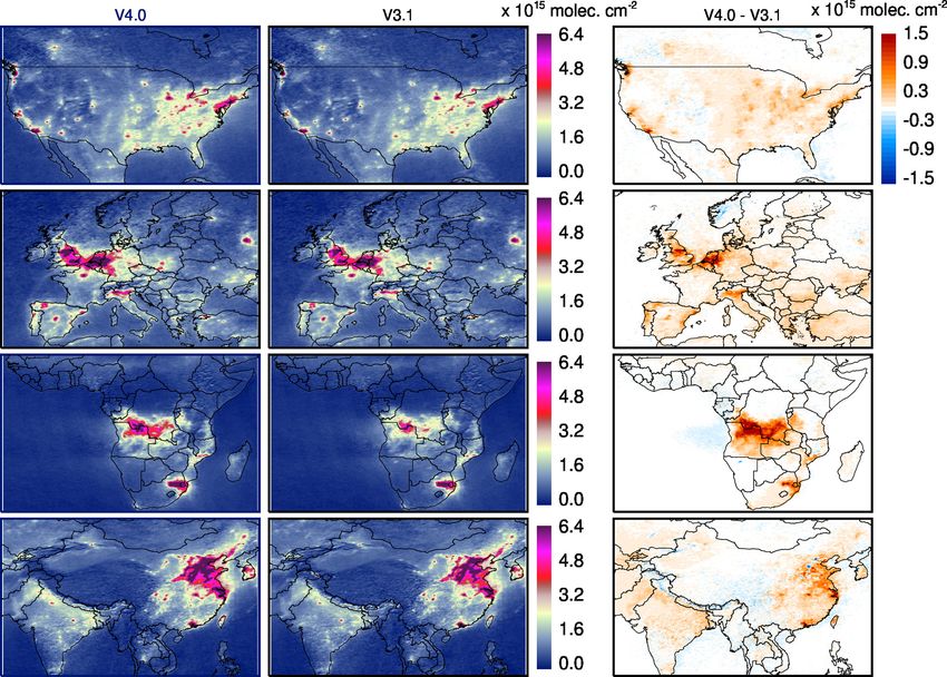
458                                             L. N. Lamsal et al.: OMI Aura nitrogen dioxide standard product version 4.0

Table 1. Summary of algorithms and approaches used in the NASA NO2 algorithms versions 3.1 and 4.0.

             Algorithm component                Version 3.1 (released 2018)                  Version 4.0 (released 2019)
   Spectral fit   NO2                           Modified DOAS fit                            Same as in V3.1
                                                (Marchenko et al., 2015)
                  O2 –O2                        DOAS fit from KNMI                           Modified DOAS fit
                                                (Veefkind et al., 2016)                      (Vasilkov et al., 2018)
   AMF            Terrain reflectivity          Monthly climatology                          Daily GLER data (Vasilkov et al., 2017;
                                                (Kleipool et al., 2008)                      Qin et al., 2019; Fasnacht et al., 2019)
                  Terrain pressure              At pixel center (calculated from terrain     Average over pixel (calculated from
                                                height and GMI terrain pressure)             terrain height and GMI terrain pressure)
                  Cloud pressure and fraction   Operational O2 –O2 cloud product             New O2 –O2 cloud product
                                                (OMCLDO2) v2.0 (Veefkind et al., 2016)       (OMCDO2N) derived using the
                                                                                             GLER product (Vasilkov et al., 2018)
                  Cloud radiance fraction       Calculated at 440 nm from OMCLDO2            Calculated at 440 nm from OMCDO2N
                                                v2.0 cloud fraction using VLIDORT-           cloud fraction using VLIDORT-based
                                                based lookup table                           lookup table
                  Scattering weights            TOMRAD-based lookup table                    Same as in V3.1
                  A priori NO2 profiles         GMI-derived yearly varying monthly           Same as in V3.1
                                                mean profiles at 1◦ × 1.25◦
   Stripe correction                            Based on data from 30◦ S–5◦ N of five        Same as in V3.1
                                                orbits
   Stratosphere–troposphere separation          Spatial filtering and interpolation          Same as in V3.1
                                                (Bucsela et al., 2013), but with
                                                minor changes in box sizes

represents the integrated abundance of NO2 along the aver-                //www.qa4ecv.eu/, last access: 18 May 2020), BIRA-IASB’s
age photon path from the sun through the atmosphere to the                (Royal Belgian Institute for Space Aeronomy) QDOAS soft-
satellite. The Ring spectra are calculated as a linear combi-             ware (http://uv-vis.aeronomie.be/software/QDOAS/, last ac-
nation of the atmospheric (Joiner et al., 1995) and liquid wa-            cess: 18 May 2020), and the latest KNMI retrievals (van Gef-
ter (Vasilkov et al., 2002) RR spectra, convolved with the                fen et al., 2015) and are shown to agree within 2 % (Zara
wavelength- and cross-track-dependent OMI transfer func-                  et al., 2018). The typical NO2 SCD uncertainties amount
tion (Dirksen et al., 2006). The algorithm employs a multi-               to ∼ 0.8 × 10¹⁵ molec. cm−2 , or 5 %–7 % in high-SCD areas
step, iterative retrieval procedure for removal of the Ring and           and 15 %–20 % in low-SCD areas (Marchenko et al., 2015).
spectral under-sampling (Chance, et al., 2005) patterns as
well as a low-order polynomial smoothing prior to estimation              2.1.2   O2 –O2 spectral fitting algorithm
of SCDs for all interfering species. This is in contrast to the
conventional DOAS approach that treats the Ring effect as                 The oxygen dimer (O2 –O2 ) slant column fitting algorithm
a pseudo-absorber and fits all absorbers simultaneously with              shares many features of the NO2 fitting algorithm and is de-
the polynomial functions. For accurate wavelength shifts (ra-             scribed in detail in Vasilkov et al. (2018). It consists of a
diances vs. irradiances), the standard product algorithm splits           multi-step, iterative retrieval approach with three carefully
the entire fitting window into seven carefully selected, par-             selected micro-windows sampling the flanks and the core
tially overlapping micro-windows, iteratively evaluates the               of the broad O2 –O2 feature centered at 477 nm. The algo-
RR spectrum amplitudes, performs wavelength adjustments                   rithm exploits OMI-measured reflectance spectra in the 451–
for each segment, and then iteratively retrieves the NO2 ,                496 nm range to determine the wavelength shifts and RR am-
H2 O, and glyoxal in the windows best suited for a particu-               plitudes. The Ring patterns are removed from the original
lar trace gas species.                                                    OMI reflectances during the iterative adjustments for differ-
   The OMI NO2 SCDs from the standard product were                        ences in the wavelength registration of radiances and irradi-
compared with improved SCD retrievals from the Quality                    ances. The O2 –O2 slant columns are retrieved after removal
Assurance for Essential Climate Variables (QA4ECV; http:                  of the NO2 and H2 O absorptions estimated by the algorithm
                                                                          discussed in the previous section and of the ozone absorp-

Atmos. Meas. Tech., 14, 455–479, 2021                                                       https://doi.org/10.5194/amt-14-455-2021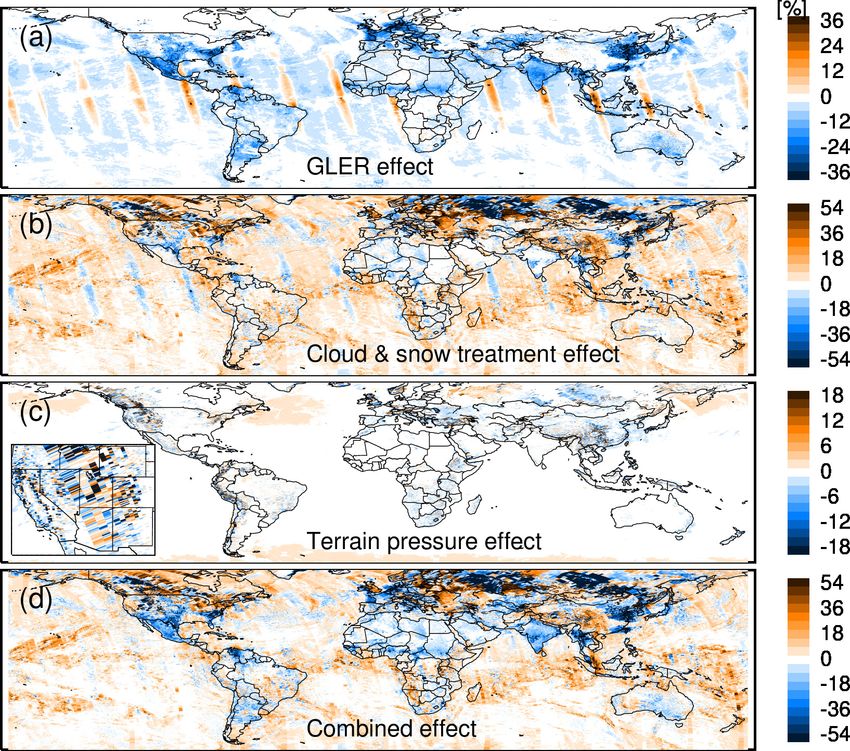
L. N. Lamsal et al.: OMI Aura nitrogen dioxide standard product version 4.0                                                    459

tion using total ozone data from Veefkind et al. (2006). Af-       resolution of the model is 1.25◦ in longitude and 1.0◦ in lat-
ter removal of the interfering signals, the 477 nm O2 –O2 ab-      itude, and the atmosphere is divided into 72 pressure levels
sorption profile is carefully normalized to the adjacent O2 –      extending from the surface to 0.01 hPa. The model output
O2 absorption-free reflectance levels accounting for very dif-     is sampled between 13:00 and 14:00 local time, consistent
ferent wavelength dependencies of surface reflectances over        with the OMI overpass time. The use of monthly NO2 pro-
various geographical sites (e.g., the open-ocean and desert        files helps capture the seasonal variation in the NO2 vertical
area), as described in Vasilkov et al. (2018). The normal-         distribution (Lamsal et al., 2010). The simulation is based
ized O2 –O2 absorption profiles are then iteratively fitted with   on yearly varying NOx emissions, as discussed in Strode
the temperature-dependent cross sections from Thalman and          et al. (2015); this is necessary to account for the effect of
Volkamer (2013) over the 463–488 nm range to derive O2 –           rapidly changing NOx emissions (e.g., Tong et al., 2015;
O2 SCDs. These are used to estimate the cloud properties as        Duncan et al., 2016; Miyazaki et al., 2017) on local NO2
discussed below in Sect. 2.2.2.                                    profile shapes (Lamsal et al., 2015; Krotkov et al., 2017).
                                                                      For each FOV, AMFs are computed for clear (AMFclr ) and
2.2   Improved air mass factor calculations                        cloudy (AMFcld ) conditions. The AMF of a partially cloudy
                                                                   scene is calculated by assuming the independent pixel ap-
The AMF, which is defined as the ratio of SCD to VCD, is           proximation:
needed to calculate the retrieved NO2 VCD. Details of the
AMF and its calculation are given in Palmer et al. (2001).         AMF = (1 − fr ) × AMFclr + fr × AMFcld ,                    (2)
The AMF for each FOV is calculated by combining altitude-
dependent (z-dependent) scattering weights (w) computed            where fr is the cloud radiance fraction (CRF), defined as the
with a radiative transfer model and a local a priori verti-        fraction of the measured radiation that comes from clouds
cal NO2 profile shape (S), taken from a chemistry transport        and scattering aerosols, and it is computed at 440 nm from
model:                                                             the retrieved effective cloud fraction (ECF), fc , using Eq. (8)
                                                                   (see below). AMFclr is calculated for the ground reflectivity
        Zz2
                                                                   of Rs and at terrain pressure Ps , whereas AMFcld is calcu-
AMF =         w (z) S (z) dz.                               (1)    lated assuming a Lambertian surface of reflectivity 0.8 at the
        z1                                                         retrieved cloud pressure. Below we provide a detailed discus-
                                                                   sion of each of these input parameters that are incorporated
For the tropospheric AMF, the integral extends from the
                                                                   in the OMNO2 V4.0 algorithm.
surface to the tropopause, whereas the integral from the
tropopause to the top of the atmosphere provides the strato-       2.2.1   New surface reflectivity product for NO2 and
spheric AMF. The scattering weight at a given altitude de-                 cloud retrievals
scribes the sensitivity of the backscattered radiation to the
abundance of the absorber at that altitude. For an optically       Surface reflectivity is an important input parameter for UV–
thin absorber like NO2 , scattering weights are a function         Vis satellite retrievals of trace gases and cloud information.
of atmospheric scattering and are considered to be inde-           The surface reflectance over both ocean and land depends
pendent of the species’ vertical distribution (Palmer et al.,      upon viewing and illumination geometry and can be accu-
2001). Factors affecting scattering weights include wave-          rately described by the bidirectional reflectance distribution
length, optical geometry (solar and viewing azimuth and            function (BRDF). This effect is, however, neglected by most
zenith angles), surface reflectivity, and cloud pressure and       currently available trace gas and cloud algorithms, which use
fraction. The wavelength dependence of scattering weights          a climatological Lambert equivalent reflectivity (LER) for
is accounted for by creating an average of scattering weights      the surface. To account for surface BRDF effects in the NO2
derived from the values at multiple wavelengths within the         and cloud retrievals, here we use the geometry-dependent
NO2 spectral fitting window. To compensate for the effect          surface LER (GLER) product derived using the Moderate
of the assumed constant NO2 temperature (220 K) in the             Resolution Imaging Spectroradiometer (MODIS) BRDF data
NO2 SCD retrievals, the scattering weights are corrected for       and the vector linearized discrete ordinate radiative transfer
the atmospheric temperature effect using local climatologi-        (VLIDORT) calculation (Vasilkov et al., 2017; Qin et al.,
cal monthly temperature profiles as discussed in Bucsela et        2019; Fasnacht et al., 2019). The GLER allows for a com-
al. (2013). These profiles are based on the meteorological         putationally efficient approach that does not require major
field from the Modern-Era Retrospective Analysis for Re-           changes to the existing trace gas and cloud algorithms.
search and Applications (MERRA-2) (Gelaro et al., 2017).              We derive GLER by inverting the top-of-atmosphere
   The a priori NO2 profile shapes are computed from a             (TOA) radiance (I ) of a Rayleigh atmosphere over a non-
monthly mean climatology of vertical NO2 profiles con-             Lambertian surface for each specific FOV and sun–satellite
structed from the Global Modeling Initiative (GMI) CTM             geometry within the Lambertian framework, i.e.,
simulation (Douglass et al., 2004; Strahan et al., 2007; Strode
et al., 2015) driven by MERRA-2 meteorology. The spatial           I = I0 + GLER × T /(1 − GLER × Sb ),                        (3)

https://doi.org/10.5194/amt-14-455-2021                                                Atmos. Meas. Tech., 14, 455–479, 2021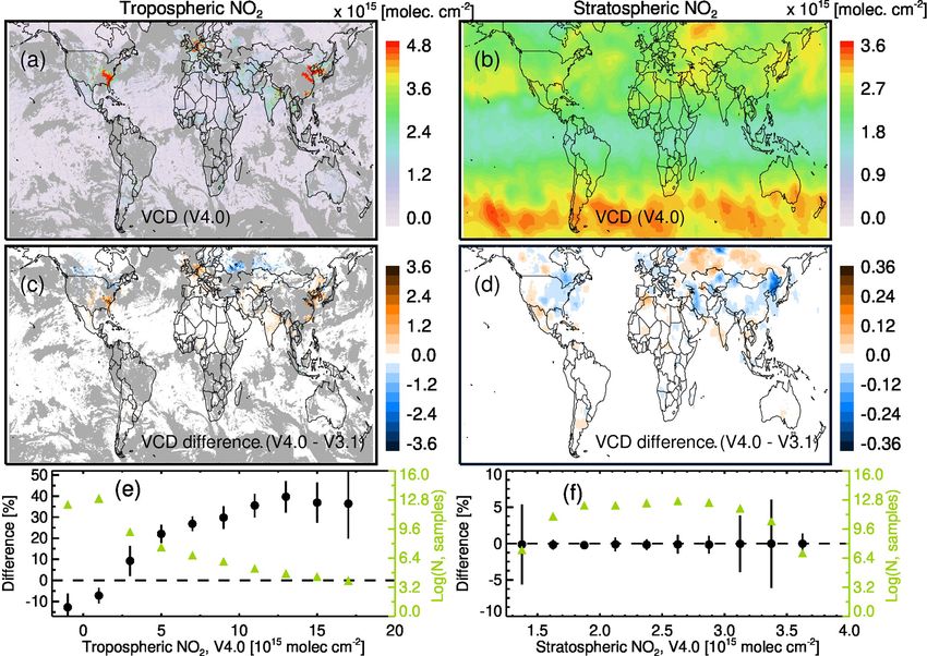
460 L. N. Lamsal et al.: OMI Aura nitrogen dioxide standard product version 4.0
where I0 is the TOA radiance calculated for a black surface, the wind direction (Cox and Munk, 1954). Polarization at the
T is the total (direct + diffuse) solar irradiance reaching the ocean surface is accounted for by using a full Fresnel reflec-
surface converted to the ideal Lambertian-reflected radiance tion matrix as suggested by Mishchenko and Travis (1997).
(by dividing by π steradians) and then multiplied by the We use wind speed data from a pair of satellite microwave
transmittance of the reflected radiation between the surface imagers that include the Advanced Microwave Scanning
and TOA in the direction of a satellite instrument, and Sb is Radiometer–Earth Observing System (AMSR-E) instrument
the diffuse flux reflectivity of the atmosphere for the case of onboard the NASA Aqua satellite (Meissner and Wentz,
its isotropic illumination from below (Dave, 1978). The val- 2004) for 2004–2011 and the Special Microwave Imager–
ues of I0 , T , and Sb are pre-computed with VLIDORT and Sounder (SSMIS) onboard the Air Force Defense Meteoro-
stored in a lookup table. The GLER values are calculated logical Satellite Program (DMSP) Satellite F16 (Wentz et
at wavelengths relevant for both NO2 (440 nm) and cloud al., 2012) afterwards. Wind direction data are taken from
(466 nm) retrievals. the Global Modeling Assimilation Office (GMAO) Goddard
Over land, the BRDF is calculated using the Ross-thick Li- Earth Observing System Model Forward Processing for In-
sparse kernel model (Lucht et al., 2000) in VLIDORT (Spurr, strument Teams (GEOS-5 FP-IT) near-real-time assimila-
2006): tion.
Diffuse light from the ocean is described by a Case 1 water
BRDF = aiso + avol kvol + ageo kvol , (4) model with a single input parameter of chlorophyll concen-
tration (Morel, 1988) taken from the monthly Aqua MODIS
where the coefficients aiso , avol , and ageo come from the
data. The common Case 1 water model developed for the vis-
Moderate Resolution Imaging Spectroradiometer (MODIS)
ible channel (Morel, 1988) was extended to the UV using
Collection 5 gap-filled seasonally snow-free BRDF product
data from Vasilkov et al. (2002, 2005). To calculate water-
MCD43GF (Schaaf et al., 2002, 2011) for band 3 (459–
leaving radiance, we require the downwelling irradiance at
479 nm) available at 30 arcsec spatial resolution and 8 d tem-
the surface (i.e., atmospheric transmittance). Since the trans-
poral resolution. The term aiso is the isotropic contribution
mittance and the water-leaving contribution are coupled, we
describing the Lambertian part of light reflection from the
develop a simple coupling scheme in VLIDORT to ensure
surface; the volumetric kernel (kvol ) describes light reflection
that the value of water-leaving radiance used as an input at
from a dense leaf canopy, and the geometric kernel (kgeo ) de-
the ocean surface will correspond to the correct value of the
scribes light reflection from a sparse ensemble of surface ob-
downwelling flux reaching the surface interface (Fasnacht et
jects casting shadows on the background assumed to be Lam-
al., 2019).
bertian. The kernels are the only angle-dependent functions,
For OMI ground pixels covering land and water surfaces,
the expressions of which are given in Lucht et al. (2000). The
the TOA radiance (I ) is calculated as an average of radiance
band 3 BRDF coefficients spatially averaged over an actual
for land (IL ) and water (Iw ) weighted by the pixel land frac-
satellite FOV are used to calculate TOA radiance and GLER
tion (f ):
at 466 nm. To calculate GLER at 440 nm, we apply a scaling
method using the ratio of OMI-derived Lambert equivalent I = f IL + (1 − f )Iw . (6)
reflectivity (LER) data at 440 and 466 nm:
The value of f is determined by converting various surface
GLER440 = GLER466 × fs . (5) categories in the MODIS data (note that these are of much
higher spatial resolution than the OMI data) into a binary
The value of fs = LER 440
LER466 is taken from the gridded monthly land–water mask (e.g., treating all shorelines and ephemeral
LER ratio data at 1◦ × 1◦ or coarser resolution. The LER is water as the land category and classifying all other water sub-
determined from OMI TOA radiance measurements as dis- categories simply as water). The areal fraction of land (or
cussed in Vasilkov et al. (2017, 2018). We use clear-sky (ef- water) for each OMI pixel is then computed as the statistics
fective cloud fraction < 0.02) and aerosol-free (OMI UV of the binary categories.
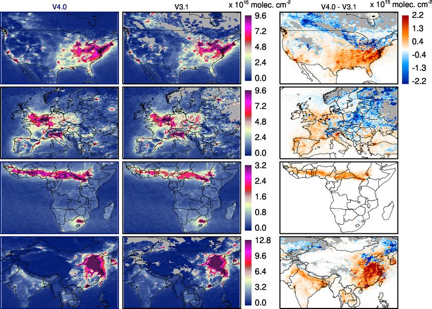
aerosol index, < 0.5; Torres et al., 2007) OMI LER data Figure 2 shows an example of changes in surface reflec-
to create the monthly gridded data. The cloud and aerosol tivity used in the previous (V3.1) and the current (V4.0) ver-
screening is necessary because the spectral dependence of sion of the OMI NO2 algorithm. The GLER data computed
surface features differs from that of clouds and aerosols. for OMI observations as discussed above for 20 March 2005
Over water, the surface reflectance is calculated at the two differ considerably from the OMI-derived climatological
wavelengths, 440 and 466 nm, using VLIDORT. To calculate monthly LER data (Kleipool et al., 2008) for March. As
TOA radiance, we include light specularly reflected from a shown in Figs. 2 and 3a, the GLERs are generally lower than
rough water surface and diffuse light backscattered by water climatological LER data except at swath edges with large
bulk. We also account for contributions from oceanic foam viewing angles and over areas affected by sun glint that cor-
that can be significant for high wind speeds. Reflection from respond to higher values of GLER. Changes over the sun-
the water surface is described by the Cox–Munk slope distri- glint areas are rather large, reaching up to 0.3. The climato-
bution function, which depends on both the wind speed and logical LER data derived by analyzing histograms of 5 years
Atmos. Meas. Tech., 14, 455–479, 2021 https://doi.org/10.5194/amt-14-455-2021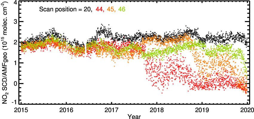
L. N. Lamsal et al.: OMI Aura nitrogen dioxide standard product version 4.0                                                   461

                                                                   Im = Ig (1 − fc ) + Ic fc .                                (7)

                                                                   We choose the wavelength of 466 nm that is not substan-
                                                                   tially affected by rotational Raman scattering (RRS) or atmo-
                                                                   spheric absorption to derive fc . The parameters Ig and Ic are
                                                                   a function of the ground and cloud LERs, respectively, and
                                                                   are calculated using VLIDORT (Spurr, 2006) and obtained
                                                                   with an interpolated lookup table. We use GLER discussed
                                                                   above for ground reflectivity and a uniform cloud reflectiv-
                                                                   ity of 0.8 (Koelemeijer et al., 2001; Stammes et al., 2008).
                                                                   The value of fc is calculated by inverting Eq. (7). Note that
                                                                   aerosols are implicitly accounted for in the determination of
                                                                   fc , as they are treated (like clouds) as particulate scatters.
Figure 2. Surface reflectivity at 440 nm (a) derived using MODIS   CRF (fr ) defines the fraction of TOA radiance reflected by
BRDF data with OMI geometry (GLER) on 20 March 2005 com-           cloud:
pared with (b) OMI-based monthly LER climatology (OMLER) for                   Ic
the month of March (Kleipool et al., 2008). The bottom panel (c)   fr = fc ×      .                                           (8)
shows the difference between MODIS-based and climatological                    Im
surface reflectivity data.
                                                                   We use pre-computed lookup tables of the TOA radiances
                                                                   generated using VLIDORT. Due to its wavelength depen-
of OMI-based LER data likely overestimate the actual sur-          dence, we calculate CRF at 466 nm for OCP at 440 nm for
face reflectivity due to residual cloud and aerosol contami-       NO2 retrievals.
nation and underestimate over sun-glint areas as the proce-           The MLER model compensates for photon transport
dure ignores sun-glint-affected observations. In contrast, the     within a cloud by placing the Lambertian surface somewhere
GLER data over land are based on atmospherically corrected         in the middle of the cloud instead of at the top (Vasilkov
radiances from high-resolution MODIS observations, mini-           et al., 2008). The pressure of this surface corresponds to
mizing the impact of both cloud and aerosols.                      OCP, which can be modeled as a reflectance-averaged pres-
                                                                   sure level reached by backscattered photons (Joiner et al.,
2.2.2   Improved cloud product retrieval                           2012). We retrieve cloud OCP from the O2 –O2 SCD dis-
                                                                   cussed above (Sect. 2.1.2). The cloud OCP, Pc , is estimated
We develop a new algorithm that provides cloud parame-             by inversion using the MLER method to compute the appro-
ters, namely cloud radiance fraction (CRF) and cloud opti-         priate O2 –O2 AMFs:
cal centroid pressure (OCP), and use them in the OMNO2
algorithm. Similar to the standard OMCLDO2 algorithm               SCD = AMFg ×VCDg ×(1 − fr )+AMFc ×VCDc ×fr , (9)
(Veefkind et al., 2016), our cloud algorithm exploits the
O2 –O2 absorption to retrieve O2 –O2 SCD as discussed in           where VCD (SCD / AMF) is the vertical column density of
Sect. 2.1.2, but it derives the two cloud parameters using the     O2 –O2 over ground (VCDg ) and cloud (VCDc ). The clear-
GLER and other ancillary data that are used in the NO2 al-         sky (AMFg ) and overcast or cloudy (AMFc ) subpixel AMFs
gorithm, maintaining inter-algorithm consistency. The OM-          are calculated at 477 nm with ground (GLER) and cloud (0.8)
CLDO2 algorithm retrieves these parameters using the cli-          reflectivity, respectively. Lookup tables for the AMFs were
matological LER data from Kleipool et al. (2008). In the fol-      generated using VLIDORT. Temperature profiles needed for
lowing, our new cloud product is referred to as OMCDO2N.           estimation of VCD and AMF are taken from the GEOS-5
   The derivation of CRF and OCP is based on a simple cloud        global data assimilation system (Rienecker et al., 2011).
model called the mixed Lambertian equivalent reflectivity             In addition to OCP, we retrieve the so-called scene pres-
(MLER) model (Joiner and Vasilkov, 2006; Veefkind et al.,          sure. The scene pressure is derived from Eq. (9) assuming
2016). The MLER model treats cloud and ground as horizon-          that fr = 1 and cloud reflectivity equals the scene LER. The
tally homogeneous, opaque Lambertian surfaces and mixes            scene LER is determined from the measured TOA radiance
them using the independent pixel approximation (IPA). Ac-          using the equation (Eq. 3) that defines TOA radiance in the
cording to the IPA, the measured TOA radiance, Im , is a           Rayleigh atmosphere over a Lambertian surface. In the ab-
sum of the clear-sky (Ig ) and overcast (Ic ) subpixel TOA         sence of clouds, aerosols, and any major gas absorptions, the
radiances that are weighted with an effective cloud fraction       scene pressure should be equal to the surface pressure. The
(ECF), fc (e.g., Stammes et al., 2008):                            scene pressure is therefore an important diagnostic tool for
                                                                   evaluation of the performance of cloud pressure algorithms.

https://doi.org/10.5194/amt-14-455-2021                                                  Atmos. Meas. Tech., 14, 455–479, 2021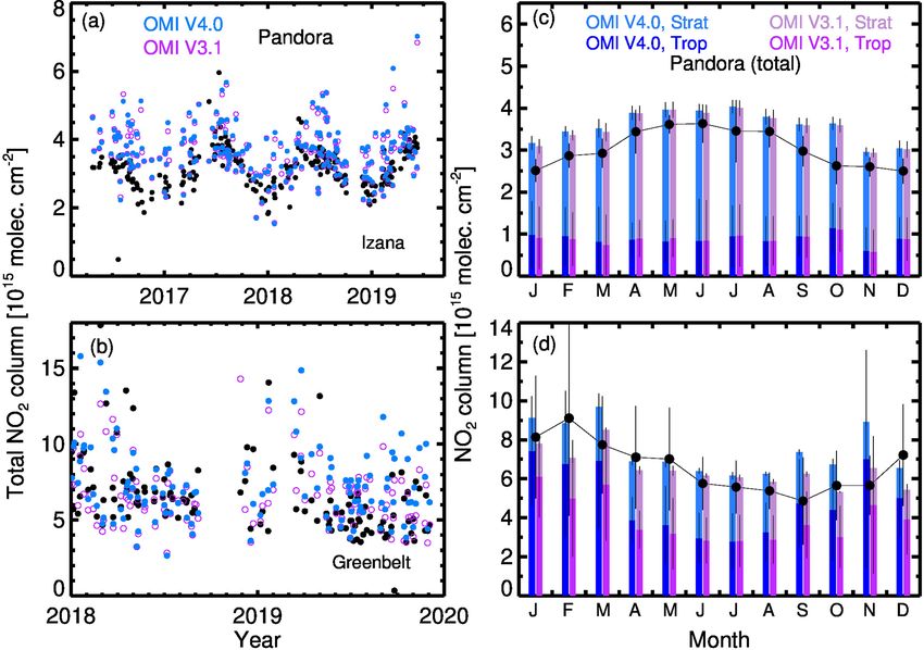
462                                             L. N. Lamsal et al.: OMI Aura nitrogen dioxide standard product version 4.0

Figure 3. Differences (V4.0–V3.1) in (a) surface reflectivity, (b) cloud radiance fraction, and (c) cloud optical centroid pressure for
20 March 2005, as used in the V3.1 and V4.0 algorithms and binned by the values of corresponding parameters from V4.0. Data are
separated for land (blue) and ocean surfaces, as well as by sun-glint (green) and non-sun-glint (orange) geometry over ocean. The vertical
bars represent the standard deviation for each bin of those parameters.

   Figure 4 shows an example of cloud products retrieved
with our algorithm compared with those retrieved from the
standard OMCLDO2 algorithm (Veefkind et al., 2016). The
retrieved OCP and CRF from the two algorithms exhibit
broadly consistent spatial patterns in both cloud altitude and
amount. The values of OCP generally range from 370 to
1001 hPa in OMCDO2N versus 150 to 1011 hPa in OM-
CLDO2N. For both products, CRF varies from 0 for clear-
sky to 1 for overcast conditions. A systematic difference
is evident, with generally higher values in OMCDO2N for
OCP by 147 hPa and CRF by 0.01 compared to OMCLDO2.
For OCP, there is a general pattern in difference, with OM-
CDO2N OCP higher for low-altitude clouds (> 700 hPa) and
lower values for high-altitude clouds (< 300 hPa) (Fig. 3c).
The largest OCP differences occur for cases in which cloud
pressures in OMCLDO2 are clipped to 150 hPa. For CRF,                  Figure 4. Cloud optical centroid pressure at 477 nm (a, c,
larger differences occur for partially cloudy scenes, with             e) and cloud radiance fraction at 440 nm (b, d, f) retrieved for
higher CRF values in OMCDO2N by 0–0.1 for both land and                20 March 2005 with the OMNO2 V4.0 (a, b) and V3.1 (c, d) al-
                                                                       gorithms, respectively. Panels (e, f) show their differences. Gray
water surfaces (Fig. 3b). Exceptions are over sun-glint areas
                                                                       represents the OMI pixels with retrieved cloud pressure equal to
where CRF in OMCDO2N is lower by 0–0.3 with a mean
                                                                       terrain pressure in V4.0 on the left and over snow and ice surface
difference of 0.13.                                                    identified by the NISE flag on the right.
2.2.3   Treatment over snow and ice surfaces

Over ice and snow surfaces, identified by near-real-time ice              The OMI-derived scene reflectivity and scene pressure are
and snow extent (NISE) flags (Nolin et al., 2005) in the OMI           used for NO2 and cloud retrievals over seasonally snow-
Level-1b data, the following treatments are made for surface           covered areas. If the NISE flags are set as true, the following
reflectivity. In the case of permanent ice and snow surfaces,          assumptions are made in our CRF, OCP, and NO2 retrievals.
the MCD43GF product provides BRDF parameters, allow-                   Over bright surfaces (scene reflectivity > 0.2), we consider
ing us to calculate GLER. Over seasonal snow area usually              the scenes to be snow- or cloud-covered and assign the scene
with data gaps in MCD43GF, we calculate OMI-derived LER                pressure to OCP. In addition, if the difference between the
capped by a constant snow albedo of 0.6 following Boersma              surface pressure and scene pressure is smaller than 100 hPa,
et al. (2011). In rare cases of pixels not flagged by NISE             the scene is considered to be either cloud-free or covered by
and gaps in MODIS data, we use OMI LER climatology                     optically thin clouds following the cloud over snow classi-
(Kleipool et al., 2008) regardless of whether the surface is           fication by Vasilkov et al. (2010), and CRF for the pixel is
either snow- and ice-covered but missed by NISE or snow-               set to zero. If the difference between the surface pressure and
and ice-free.                                                          scene pressure exceeds 100 hPa, the scene is considered to
                                                                       be overcast by optically thick (shielding) clouds (Vasilkov

Atmos. Meas. Tech., 14, 455–479, 2021                                                      https://doi.org/10.5194/amt-14-455-2021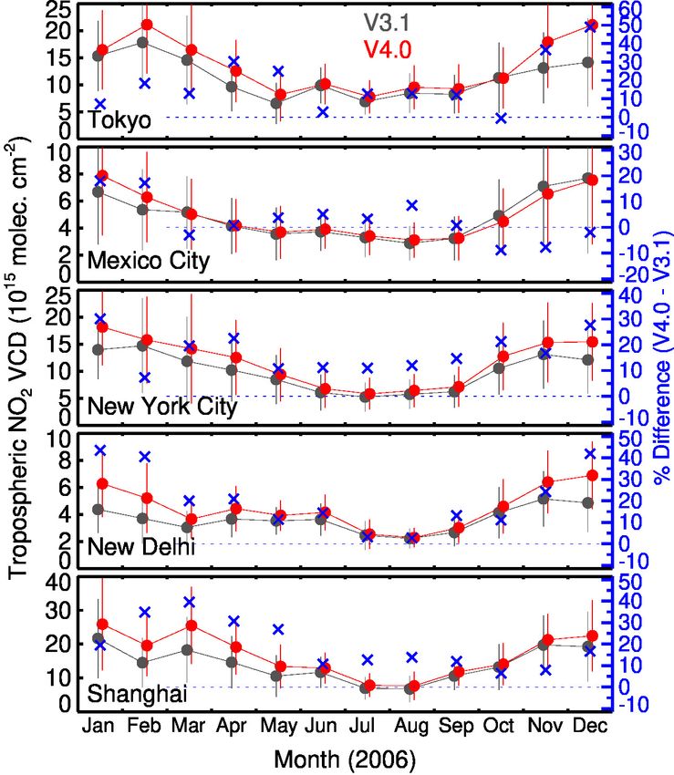
L. N. Lamsal et al.: OMI Aura nitrogen dioxide standard product version 4.0                                                        463

et al., 2010), and CRF for the pixel is set to 1. To avoid
a possible NISE misclassification (Cooper et al., 2018) for
low-reflectivity scenes (scene reflectivity < 0.2), we consider
such scenes to be snow- and ice-free and calculate CRF, OCP,
and NO2 AMF using the standard procedure with GLER for
those scenes.

2.2.4    Improved terrain height and pressure calculation

Terrain pressure is a critical parameter for the AMF in NO2
and cloud algorithms as well as for the total optical depth of
the Rayleigh atmosphere in the GLER algorithm. Prior stud-
ies have shown that errors in terrain pressure can introduce
over 20 % errors in retrieved NO2 VCD, especially in areas
of complex terrain (Zhou et al., 2010; Russell et al., 2011).
   Here, we use a 2 arcmin global relief model of global land–
water surface data (ETOPOv2; National Geophysical Data
Center, 2006) to derive terrain height for each individual
OMI ground pixel. We derive the pixel-average terrain height
by collocating and averaging the high-resolution data as dis-      Figure 5. Impact on tropospheric AMF (i.e., V4.0–V3.1) from
                                                                   changes in (a) surface reflectivity, (b) cloud and surface treatment,
cussed in Qin et al. (2019). The corresponding terrain pres-
                                                                   (c) terrain pressure, and (d) their combination on 20 March 2005.
sure for each OMI pixel (Ps ) is calculated from the terrain
                                                                   The panel (c) inset shows a zoomed view of the impact over com-
pressure–height relationship established based on MERRA-2          plex terrain in the western US.
monthly terrain pressure (Ps_GMI ) at a spatial resolution of 1◦
latitude × 1.25◦ longitude used in the GMI model discussed
above:                                                             amounts. For 80 % of cases over land, 97 % over water out-
                −( 1z
                   H )
                                                                   side sun-glint areas, and 98 % over sun-glint areas, tropo-
Ps = Ps_GMI e            ,                                 (10)
                                                                   spheric NO2 columns are < 1.5 × 10¹⁵ molec. cm−2 , and the
where 1z (= z −zGMI ) represents the difference between the        average GLER-driven differences are small at −6.6±17.3 %,
average terrain height for an OMI pixel (z) and the terrain        −3.8±7.1 %, and 4.0±12.9 %, respectively. The differences
height at GMI resolution (zGMI ). The parameter H = Mg      kT     increase gradually with column amount over NOx source re-
represents the scale height, where k is the Boltzmann con-         gions (e.g., cities and highly polluted coastal areas), with
stant, T is the temperature at the surface, M is the mean          binned (of size 1 × 10¹⁵ molec. cm−2 ) average differences
molecular weight of air, and g is the acceleration due to grav-    ranging from −10±20.1 % to −30±19.7 %. Over snow and
ity.                                                               ice surfaces, changes are rather large, reaching up to a factor
                                                                   of 2. The impact of change in the surface reflection data on
2.3     Impact of the changes on AMF                               stratospheric AMFs is negligible (< 2 %).
                                                                      Figures 5b and 6b show how changes in the cloud pa-
Figure 5 shows an example of how changes in each individ-          rameters (CRF and OCP) affect tropospheric AMF. Replac-
ual input parameter affect tropospheric AMFs, which, in turn,      ing OMCLDO2-based cloud parameters with those from
translate inversely to tropospheric NO2 column retrievals.         OMCDO2N changes scattering weight profiles in a compli-
Replacing climatological LER from OMLER with daily                 cated way. Higher values of OCP in OMCDO2N will in-
GLER data affects scattering weight profiles in the lower tro-     clude additional portions of scattering weights between the
posphere, resulting in lower values of tropospheric AMF al-        OMCDO2N- and OMCLDO2-based OCPs, especially in the
most everywhere, except over sun-glint areas where the use         lower troposphere, thereby reducing the tropospheric AMF.
of GLER enhances scattering weights and tropospheric AMF           On the other hand, the higher CRF values lead to an in-
(Fig. 5a). The changes in tropospheric AMF with GLER usu-          creased contribution of the cloudy AMF in the calculation of
ally range from −50 % to 25 %, occasionally reaching up            tropospheric AMF, thereby increasing its value. Their com-
to −100 %. The effect is small (−6 % to 1 %) for overcast          bination causes a wide range of scenarios and large vari-
scenes (CRF > 0.9), increases (−28 % to 17 %) over clear           ation in the AMF effect. Overall, the change in cloud pa-
and partially cloudy scenes (CRF < 0.5) for unpolluted re-         rameters causes enhancement of tropospheric AMFs for par-
gions, and surges (−62 % to 3 %) over polluted areas (> 5 ×        tially cloudy and overcast scenes and reduction for clear-sky
1015 molec. cm−2 ). Figure 6a shows GLER-driven changes            scenes, especially over polluted areas. The AMF differences
in clear-sky (CRF < 0.5) tropospheric AMF for different sur-       are generally large for low AMF values that are driven by
face and scene types, separated by tropospheric NO2 column         enhanced differences in either OCP, CRF, or both as dis-

https://doi.org/10.5194/amt-14-455-2021                                                  Atmos. Meas. Tech., 14, 455–479, 2021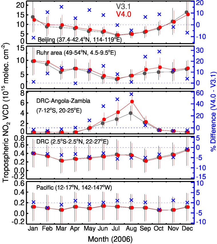
464                                            L. N. Lamsal et al.: OMI Aura nitrogen dioxide standard product version 4.0

cussed in Vasilkov et al. (2017). The changes in tropospheric       estimates the mean cross-track biases using measurements
AMF with the OMCDO2N-based cloud parameters usually                 obtained at latitudes between 30◦ S and 5◦ N and from orbits
range from −17 % to 28 %, with larger variation over land           within two orbits of the target orbit. These correction values,
(−34 % to 40 %) compared to water (−12 % to 25 %) and               one for each cross-track position, are then subtracted from
for low (< 1) AMF (−47 % to 41 %) compared to high (> 3)            the retrieved SCDs to derive the de-striped SCD field.
AMF (−4 % to 18 %). The largest changes in AMF (−96 %                  Starting 25 June 2007 and presumably even earlier, OMI
to 62 %) occur over snow and ice surfaces that result from the      experienced a more severe form of anomaly that affects the
difference in the treatment of snow and ice for cloud and NO2       quality of radiance data in certain rows at all wavelengths
retrievals as discussed in Sect. 2.2.3. For clear-sky and par-      (Dobber et al., 2008; Schenkeveld et al., 2017). This effect,
tially cloudy scenes with CRF < 0.5, the effect of the changes      called the “row anomaly” (RA), has developed and changed
in cloud parameters differs between land and water surfaces         over time. Currently, the RA has affected approximately half
as well as sun-glint and non-sun-glint geometries and be-           of the OMI’s FOVs, resulting in OMI’s global coverage now
comes more pronounced over polluted land and coastal areas          being 2 d instead of 1 d before the onset of the RA.
(Fig. 6b). As in the case of surface reflectivity, the impact          The quality of radiance data for the RA-affected FOVs
of the change in cloud parameters on stratospheric AMF is           is sufficiently poor as to prevent reliable NO2 retrievals.
< 1 %.                                                              Therefore, we abandon retrieval calculations for all measure-
   Figure 5c presents an example of changes in tropospheric         ments that are flagged by the RA-detection algorithm used
AMF differences between the previous approach of using ter-         in the Level-1 processing. We found that this RA-detection
rain pressure at OMI pixel centers and the pixel-average ter-       algorithm may not be sufficiently sensitive to the relatively
rain pressure implemented in the current version (V4.0). In         small (but important for our purposes) RA changes. Figure 7
general, the AMF changes driven by the changes in terrain           shows an example of anomalous rows not flagged by the
pressure are within ±1 % over ocean and ±3 % over land,             RA-detection algorithm but observed in the NO2 retrievals.
although at times they can reach up to 30 %, especially for         Shown are time series of average NO2 SCDs normalized
observations over complex terrain such as mountainous re-           by geometric AMFs over the Pacific Ocean for the RA-
gions (Fig. 5c inset).                                              unaffected row of 20 (0-based) compared with three rows
   Figures 5d and 6c show the AMF differences arising from          that show significant degradation in the quality of SCD re-
the combined effect of changes in all parameters discussed          trievals. These particular rows are in immediate proximity to
above. The effect arising from the replacement of the cli-          the main RA area, thus showing the gradual RA evolution:
matological OMLER with GLER is partially compensated                in the present epoch the RA slowly shifts towards the high-
for by the effect arising from the change in cloud param-           numbered rows – note the sequential timing of the big drops
eters in places where the two parameters exhibit opposite           in the retrievals in rows 44–46. While the data from the three
trends. Exceptions are over polluted land and coastal ar-           rows start deviating from row 20 beginning from summer
eas; the GLER effect on AMF is augmented by the cloud               2016, the data quality degrades further for rows 44, 45, and
effect. The average AMF changes arising from all param-             46 from September of 2017, 2018, and 2019, respectively, to
eters (2 %) are lower than the changes arising from either          the extent that they cannot be sufficiently corrected by the de-
GLER (−2.3 %) or cloud parameters (4.1 %), although the             striping algorithm. In such cases, we implement additional
combined effect leads to a wider range of variation in AMF          RA flagging for those rows that start showing anomalous be-
changes (−100 % to 57 %) compared to the effect from indi-          havior and exclude those data from Level-2 and higher-level
vidual parameters. The changes arising from all parameters          NO2 products.
are somewhat smaller (−21 % to 34 %) for overcast scenes
(CRF > 0.9) compared to (−47 % to 29 %) clear and partially         2.5   Calculation of stratospheric and tropospheric NO2
cloudy scenes (CRF < 0.5) and are substantial (−137 % to                  columns
30 %) over highly polluted areas (> 5 × 10¹⁵ molec. cm−2 )
and over snow and ice surfaces (−126 % to 99 %). Differ-            We use an observation-based stratosphere–troposphere sepa-
ences in the AMF effect are evident among land, water, and          ration scheme to estimate the stratospheric NO2 field, as dis-
sun-glint areas (Fig. 6c). The impact of the changes is below       cussed in detail in Bucsela et al. (2013), and the algorithm
1 % for the stratospheric AMF.                                      remains unchanged in the current version. Briefly, the strato-
                                                                    spheric field for an orbit is computed by creating a gridded
2.4   Row anomaly and removal of stripes                            global field of initial stratospheric NO2 VCD estimates (Vinit )
                                                                    with data assembled from within ±7 orbits of the target orbit:
The retrieved NO2 SCDs have persistent relative biases in                      Sstrat    S − Stropap
the 60 cross-track FOVs and show a pattern of stripes run-          Vinit =            =             .                         (11)
                                                                              AMFstrat    AMFstrat
ning along each orbital track. This instrumental artifact is
corrected using the “de-striping” procedure described in de-        Here, Sstrat and AMFstrat represent stratospheric SCD and
tail in Bucsela et al. (2013). Briefly, the de-striping algorithm   AMF, respectively. A priori estimates of the tropospheric

Atmos. Meas. Tech., 14, 455–479, 2021                                                   https://doi.org/10.5194/amt-14-455-2021
L. N. Lamsal et al.: OMI Aura nitrogen dioxide standard product version 4.0 465
Figure 6. The impact on tropospheric AMF (i.e., V4.0–V3.1) from changes in (a) surface reflectivity, (b) cloud, and (c) their combination
for clear and partially cloudy scenes (CRF < 0.5) on 20 March 2005. Percent differences in tropospheric AMF are sorted by tropospheric
NO2 columns, separating them by land (blue) and ocean, as well as by sun-glint (green) and non-sun-glint (orange) geometry over ocean.
The vertical bars represent the standard deviations for the tropospheric NO2 column bins.
With the updates in surface and cloud treatments as dis-
cussed in Sect. 2.2, the current version has made significant
improvements, particularly in tropospheric AMFs and con-
sequently in VCD estimates. Further improvement to the re-
trievals is possible by enhancing the quality of a priori NO2
profiles through improvements in model resolution, emis-
sions, and chemistry, which remain unchanged in the current
version. If improved a priori NO2 profiles become available,
one can first use Eq. (1) to readily recalculate AMFtrop by
combining them with scattering weights (w (z)) archived in
Figure 7. The time series of OMI NO2 SCD normalized by the data files and then use Eq. (12) together with other sup-
the geometric AMF for clear-sky and partially cloudy conditions plied parameters to recalculate Vtrop . The same approach can
(CRF < 0.5) over the Pacific Ocean. The data are separated by be applied to remove the effect of a priori profiles used in
cross-track scan position, comparing the presumably RA-free row retrievals altogether, while comparing NO2 columns from a
20 (black) with rows 44 (red), 45 (orange), and 46 (green). The row model simulation with retrievals (Eskes and Boersma, 2003;
numbers are 0-based. Lamsal et al., 2014).
Figure 8 shows a comparison of tropospheric and strato-
contribution (Stropap ) are subtracted from the measured de- spheric NO2 columns retrieved from the V3.1 and V4.0
striped SCDs (S), and grid cells wherein this contribution algorithms for 20 March 2005. As expected, the updates
exceeds 0.3 × 10¹⁵ molec. cm−2 are masked. This masking implemented in V4.0 yield higher (∼ 10 %–40 %) tropo-
ensures that the model contribution to the retrieval is min- spheric NO2 columns in polluted areas, with less-pronounced
imal, especially in polluted areas. The residual field of the (±10 %) differences in background and low-column ar-
initial stratospheric VCDs measured outside the masked re- eas. These results are consistent with the observed dif-
gions mainly over unpolluted or cloudy areas is smoothed by ferences in the tropospheric AMF as discussed above in
a boxcar average and a two-dimensional interpolation, yield- Sect. 2.2.4 and with other previous regional studies over
ing an estimate for stratospheric NO2 VCD (Vstrat ) for an in- land surfaces (Zhou et al., 2010; McLinden et al., 2014;
dividual ground pixel. Lin et al., 2014, 2015; Laughner et al., 2019; Liu et al.,
The estimation of the stratospheric NO2 VCD allows for 2019) that implemented one or more of the changes ap-
the computation of the tropospheric NO2 VCD (Vtrop ) from plied in V4.0. In contrast to changes in tropospheric NO2
the de-striped NO2 SCD (S) and the tropospheric AMF retrievals, changes in stratospheric NO2 estimates range be-
(AMFtrop ): tween −3.6 × 10¹⁴ molec. cm−2 and 3.2 × 10¹⁴ molec. cm−2
and are close to the range of expected uncertainties of strato-
Strop S − Sstrat spheric NO2 estimates (Bucsela et al., 2013). The relative
Vtrop = = , (12) differences in the stratospheric NO2 column between the two
AMFtrop AMFtrop
versions are close to 0 % on average, usually ranging be-
where stratospheric NO2 SCD (Sstrat ) is calculated from tween −2.5 % and 2.0 % and occasionally reaching up to
stratospheric AMF (AMFstrat ) and Vstrat computed in the pre- ±13 %. This difference in stratospheric NO2 estimates is
vious step. much larger than the difference in stratospheric AMFs and
https://doi.org/10.5194/amt-14-455-2021 Atmos. Meas. Tech., 14, 455–479, 2021466 L. N. Lamsal et al.: OMI Aura nitrogen dioxide standard product version 4.0 is caused by differences in tropospheric AMFs that influence In Fig. 12, we examine the monthly variation of tropo- NO2 observations over unpolluted and cloudy areas used by spheric NO2 columns from the two versions over five highly the stratosphere–troposphere separation scheme. populated and polluted cities that vary in terrain types rang- Figure 9 shows the seasonally averaged tropo- ing from coastal (e.g., Shanghai, Tokyo) to mountainous spheric NO2 columns over the selected domains of (e.g., Mexico City). NO2 columns in V4.0 are generally North America, Europe, southern Africa, and Asia for the higher than V3.1 by 0 %–30 %, but the difference can oc- months of June, July, and August in 2005. These domains casionally reach up to 50 % in some months. Changes of that contain highly polluted areas with significant NOx emissions order of magnitude in highly polluted areas have implica- where the impact of changes in surface reflectivity and tions for the estimation of NOx emissions and trends using cloud parameters on tropospheric NO2 retrievals becomes these data. increasingly important. The use of more accurate pixel- specific information for surface and cloud parameters in V4.0 results in significantly enhanced tropospheric NO2 3 Assessment of OMI NO2 product column retrievals almost everywhere. The effect, however, varies with the vertical distribution of NO2 , with the largest In this section, we compare OMI NO2 columns with total effects in high-column areas. column retrievals from ground-based Pandora measurements Figure 10 shows the seasonal average tropospheric NO2 and integrated tropospheric columns from aircraft spirals at columns for December through February. While seasonal dif- several locations of the DISCOVER-AQ (Deriving Informa- ferences in NO2 columns are evident owing to changes in tion on Surface Conditions from COlumn and VERtically NOx lifetime and boundary layer depth, the impact of algo- Resolved Observations Relevant to Air Quality) field cam- rithm changes in V4.0 remains similar. There are two notable paign held between 2011 and 2014. exceptions specifically related to observations over snow and ice surfaces. First, there are significant data gaps in V3.1 3.1 Comparison between OMI and Pandora total but nearly none in V4.0. In V3.1, retrievals over snow and column NO2 ice areas were considered to be highly uncertain and there- fore discarded, following the recommendation of Boersma et Here, we compare the total column NO2 retrievals from OMI al. (2011). As discussed above in Sect. 2.2.3, V4.0 incorpo- and the ground-based Pandora spectrometer. Pandora is a rates changes in surface and cloud treatment in the NO2 algo- compact sun-viewing remote sensing instrument that pro- rithm that allows us to retain more observations that we de- vides estimates of NO2 column amounts from the surface to termine to be our acceptable level of cloudiness. Next, these the top of the atmosphere (Herman et al., 2009, 2018). The algorithm changes led to profound changes in the calculated NO2 retrieval approach for Pandora is similar to that of OMI tropospheric AMFs and resulting NO2 column amounts. The and consists of the DOAS spectral fitting procedure to derive reduction in tropospheric NO2 retrievals in V4.0 over snow- NO2 SCD and its conversion to VCD using AMFs. How- and ice-covered surfaces arises from a combined effect of en- ever, the details differ due to the lack of top-of-atmosphere hanced values of surface reflectivity, their impact on the CRF radiance measurements for the spectral fitting and simplic- and OCP retrievals, and an inconsistent number of samples ity in the AMF calculation for Pandora due to its direct-sun used in the calculation of the seasonal average. Nevertheless, measurements. due to inferiority in the quality of BRDF data and complexi- To compare with the OMI observations, we use Pan- ties in separating snow from clouds, caution is needed when dora data for sites listed in the Pandonia Global Net- interpreting wintertime data at high latitudes. work (https://www.pandonia-global-network.org/, last ac- Figure 11 shows some examples of how changes in the cess: 10 May 2020). Out of 22 sites, we select 18 sites that we algorithm from V3.1 to V4.0 affect monthly domain aver- determined to be suitable for comparison. Data from some age tropospheric NO2 columns over areas affected by vari- of the sites (e.g., Rome, Italy) are consistently higher than ous NOx sources. In contrast to minor changes over the pris- OMI by over a factor of 2, suggesting that the sites may be tine Pacific Ocean, month-to-month changes over source re- in close proximity to local sources that cannot be resolved gions vary considerably. The differences in tropospheric NO2 by OMI. Although some of the selected sites have sporadic columns between V4.0 and V3.1 range from −11 % to 15 % and short-term measurements (e.g., Ulsan, South Korea), we over Beijing, China, and from 0 % to 29 % over the Ruhr consider them for improved sampling and coverage. The col- area in Germany, suggesting variations in relative differences location criteria include spatial and temporal matching be- among cities and industrial areas. The changes over a major tween OMI and Pandora observations by selecting the OMI biomass burning area in the Democratic Republic of Congo, pixels that encompass the Pandora site and using Pandora Angola, and Zambia range 13 %–56 % during the biomass 80 s total NO2 column data averaged over ±10 min of OMI burning season of May through August but are < 5 % in other observations. We use high-quality data obtained under clear- months. Differences between the two versions are small over sky conditions with the root mean square of spectral fitting areas influenced by lightning NOx emissions. residuals < 0.05 and NO2 retrieval uncertainty < 0.05 DU Atmos. Meas. Tech., 14, 455–479, 2021 https://doi.org/10.5194/amt-14-455-2021
You can also read