Deepening roots can enhance carbonate weathering by amplifying CO2-rich recharge - BG
←
→
Page content transcription
If your browser does not render page correctly, please read the page content below
Biogeosciences, 18, 55–75, 2021
https://doi.org/10.5194/bg-18-55-2021
© Author(s) 2021. This work is distributed under
the Creative Commons Attribution 4.0 License.

Deepening roots can enhance carbonate weathering by amplifying
CO2-rich recharge
Hang Wen1 , Pamela L. Sullivan2 , Gwendolyn L. Macpherson3 , Sharon A. Billings4 , and Li Li1
1 Department  of Civil and Environmental Engineering, Pennsylvania State University,
University Park, PA 16802, United States
2 College of Earth, Ocean, and Atmospheric Science, Oregon State University, Corvallis, OR 97331, United States
3 Department of Geology, University of Kansas, Lawrence, KS 66045, United States
4 Department of Ecology and Evolutionary Biology and Kansas Biological Survey, University of Kansas,

Lawrence, KS 66045, United States

Correspondence: Li Li (lili@engr.psu.edu)

Received: 20 May 2020 – Discussion started: 9 June 2020
Revised: 8 October 2020 – Accepted: 11 October 2020 – Published: 5 January 2021

Abstract. Carbonate weathering is essential in regulating at-      CO2 data suggest relatively similar soil CO2 distribution over
mospheric CO2 and carbon cycle at the century timescale.           depth, which in woodlands and grasslands leads only to 1 %
Plant roots accelerate weathering by elevating soil CO2 via        to ∼ 12 % difference in weathering rates if flow partitioning
respiration. It however remains poorly understood how and          was kept the same between the two land covers. In contrast,
how much rooting characteristics (e.g., depth and density dis-     deepening roots can enhance weathering by ∼ 17 % to 200 %
tribution) modify flow paths and weathering. We address this       as infiltration rates increased from 3.7 × 10⁻² to 3.7 m/a.
knowledge gap using field data from and reactive transport         Weathering rates in these cases however are more than an
numerical experiments at the Konza Prairie Biological Sta-         order of magnitude higher than a case without roots at all,
tion (Konza), Kansas (USA), a site where woody encroach-           underscoring the essential role of roots in general. Numeri-
ment into grasslands is surmised to deepen roots.                  cal experiments also indicate that weathering fronts in wood-
   Results indicate that deepening roots can enhance weath-        lands propagated > 2 times deeper compared to grasslands
ering in two ways. First, deepening roots can control ther-        after 300 years at an infiltration rate of 0.37 m/a. These differ-
modynamic limits of carbonate dissolution by regulating            ences in weathering fronts are ultimately caused by the dif-
how much CO2 transports vertical downward to the deeper            ferences in the contact times of CO2 -charged water with car-
carbonate-rich zone. The base-case data and model from             bonate in the deep subsurface. Within the limitation of mod-
Konza reveal that concentrations of Ca and dissolved inor-         eling exercises, these data and numerical experiments prompt
ganic carbon (DIC) are regulated by soil pCO2 driven by            the hypothesis that (1) deepening roots in woodlands can
the seasonal soil respiration. This relationship can be encap-     enhance carbonate weathering by promoting recharge and
sulated in equations derived in this work describing the de-       CO2 –carbonate contact in the deep subsurface and (2) the
pendence of Ca and DIC on temperature and soil CO2 . The           hydrological impacts of rooting characteristics can be more
relationship can explain spring water Ca and DIC concentra-        influential than those of soil CO2 distribution in modulating
tions from multiple carbonate-dominated catchments. Sec-           weathering rates. We call for colocated characterizations of
ond, numerical experiments show that roots control weather-        roots, subsurface structure, and soil CO2 levels, as well as
ing rates by regulating recharge (or vertical water fluxes) into   their linkage to water and water chemistry. These measure-
the deeper carbonate zone and export reaction products at          ments will be essential to illuminate feedback mechanisms
dissolution equilibrium. The numerical experiments explored        of land cover changes, chemical weathering, global carbon
the potential effects of partitioning 40 % of infiltrated water    cycle, and climate.
to depth in woodlands compared to 5 % in grasslands. Soil

Published by Copernicus Publications on behalf of the European Geosciences Union.
56                                                        H. Wen et al.: Deepening roots can enhance carbonate weathering

1    Introduction                                                 ture soil aggregates that facilitate shallow, near-surface water
                                                                  flow (Oades, 1993; Nippert et al., 2012). In contrast, in shrub-
Carbonate weathering has long been considered negligible as       lands and forests, generally deeper and thicker roots tend to
a long-term control of atmospheric CO2 (0.5 to 1 Ma; Berner       promote a high abundance of macropores and high connec-
and Berner, 2012; Winnick and Maher, 2018). Recent stud-          tivity to the deep subsurface (Canadell et al., 1996; Nardini
ies, however, have underscored its significance in controlling    et al., 2016), enhancing the drainage of water to the depth
the global carbon cycle at the century timescale that is rel-     (Pawlik et al., 2016).
evant to modern climate change, owing to its rapid disso-            It is generally known that rooting characteristics vary
lution, its fast response to perturbations, and the order-of-     among plant species and are critical in regulating water bud-
magnitude-higher carbon store in carbonate reservoirs com-        gets, flow paths, and storage (Sadras, 2003; Nepstad et al.,
pared to the atmosphere (Gaillardet et al., 2019; Sullivan et     1994; Jackson et al., 1996; Cheng et al., 2011; Brunner et
al., 2019b). Carbonate weathering is influenced by many fac-      al., 2015; Fan et al., 2017). Existing studies however have
tors, including temperature (Romero-Mujalli et al., 2019b),       primarily focused on the role of soil CO2 and organic acids
hydrological regimes (Romero-Mujalli et al., 2019a; Wen           (Drever, 1994; Lawrence et al., 2014; Gaillardet et al., 2019;
and Li, 2018), and soil CO2 concentrations (Covington et al.,     Hauser et al., 2020). Systematic studies on coupled effects
2015) arising from different vegetation types (Calmels et al.,    of hydrological flow paths and soil CO2 distribution are
2014). Rapid alteration to any of these factors, either human     missing, owing to the limitation in data that detail root-
or climate induced, may change global carbonate weathering        ing effects on flow partitioning and complex hydrological–
fluxes and lead to a departure from the current global atmo-      biogeochemical interactions (Li et al., 2020). Here we ask
spheric CO2 level. This is particularly important given that      the following questions. How and to what degree do root-
about 7 %–12 % of the Earth’s continental area is carbonate       ing characteristics influence carbonate weathering when con-
based and about 25 % of the global population completely or       sidering both flow partitioning and soil CO2 distribution?
partially depend on waters from karst aquifers (Hartmann et       Which factor (flow partitioning or soil CO2 distribution) pre-
al., 2014).                                                       dominantly controls weathering? We hypothesized that deep-
   Plant roots have long been recognized as a dominant biotic     ening roots in woodlands enhance carbonate weathering by
driver of chemical weathering and the global carbon cycle         promoting CO2 -enriched recharge into the deep, carbonate-
(Berner, 1992; Beerling et al., 1998; Brantley et al., 2017a).    abundant subsurface (Fig. 1).
The growth of forests has been documented to elevate soil            We tested the hypotheses by a series of numerical experi-
pCO2 and amplify dissolved inorganic carbon (DIC) fluxes          ments of reactive transport processes based on water chem-
(Berner, 1997; Andrews and Schlesinger, 2001). Rooting            istry data from an upland watershed in the Konza Prairie
structure can influence weathering in two ways (Fig. 1). First,   Biological Station, a tallgrass prairie and one of the Long-
rooting systems (e.g., grasslands, shrublands, and wood-          Term Ecological Research (LTER) sites in the US (Fig. S1,
lands) may affect the distribution of soil carbon (both organic   Macpherson and Sullivan, 2019b; Vero et al., 2018). We
and inorganic), microbe biomass, and soil respiration (Dr-        used the calibrated model to carry out numerical experiments
ever, 1994; Jackson et al., 1996; Billings et al., 2018). The     for two end-members of vegetation covers, grasslands and
relatively deep root distributions of shrublands compared to      woodlands, under flow-partitioning conditions that are char-
grasslands may lead to deeper soil carbon profiles (Jackson       acteristic of their rooting structure. These experiments dif-
et al., 1996; Jobbagy and Jackson, 2000), which may help          ferentiated the impacts of biogeochemical and hydrological
elevate the deep CO2 and acidity that determine carbonate         drivers and bracketed the range of their potential impacts on
solubility and weathering rates.                                  weathering, thus providing insights on the missing quantita-
   Second, plant roots may affect soil structure and hy-          tive link between rooting structure and chemical weathering.
drological processes. Root trenching and etching can de-          We recognize that rooting characteristics can have multiple
velop porosity (Mottershead et al., 2003; Hasenmueller et         influences on water flow paths and the water budget, for ex-
al., 2017). Root death and decay can promote the genera-          ample, via water uptake and transpiration (Sadras, 2003; Fan
tion of macropores or, more specifically, biopores with con-      et al., 2017; Pierret et al., 2016). This study focuses primarily
nected networks (Angers and Caron, 1998; Zhang et al.,            on their potential influence via the alteration of hydrological
2015). Root channels have been estimated to account for           flow paths.
about 70 % of the total described macropores (Noguchi et
al., 1997; Beven and Germann, 2013) and for over 70 % of
water fluxes through soils (Watson and Luxmoore, 1986).
In grasslands, the lateral, dense spread of roots in upper
soil layers promotes the formation of horizontally oriented
macropores that support near-surface lateral flow (Cheng et
al., 2011). Highly dense fine roots also increase the abun-
dance of organic matter and promote granular or sandy tex-

Biogeosciences, 18, 55–75, 2021                                                         https://doi.org/10.5194/bg-18-55-2021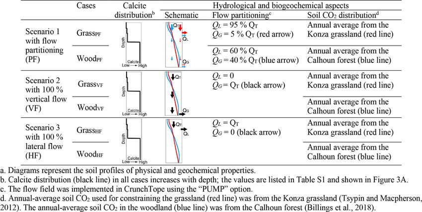
H. Wen et al.: Deepening roots can enhance carbonate weathering 57
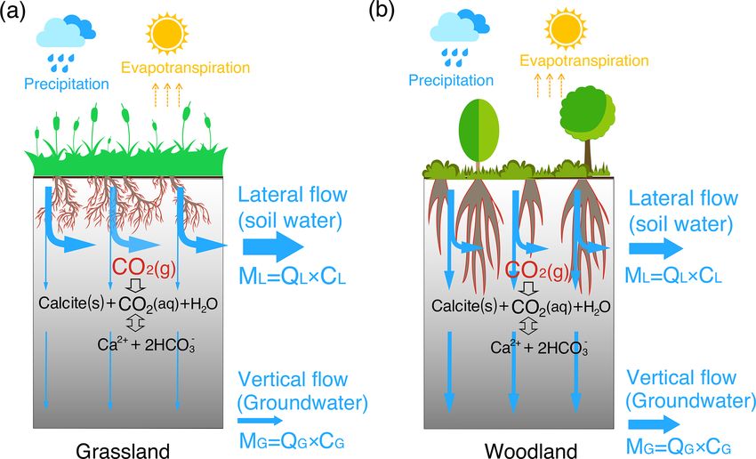
Figure 1. A conceptual diagram of hydro-biogeochemical interactions in the grassland (a) and woodland (b). The shallow and dense fine
roots in the grassland promote lateral macropore development and lateral water flow. In contrast, the woodlands induce vertical macropore
development that supports vertical flow (recharge) into the deep, calcite-abundant subsurface compared to the grassland. The gray color
gradient reflects the calcite abundance with more calcite in depth. ML and MG with a unit of moles per year (= flow rate Q (m/a) × species
concentration C (mol/m3 ) × cross-section area (m2 )) represent mass fluxes from lateral flow (soil water) and from vertical flow into ground-
water, respectively. Soil water and groundwater were assumed to eventually flow into stream, adding up to the total discharge (infiltration)
rate QT = QL + QG .
2 Research site and data sources woody-encroached sites compared to grass sites. Sullivan
et al. (2019a) hypothesized that concentration–discharge re-
2.1 Site description lationships may be affected by woody species with deeper
roots, which altered flow paths and mineral–water interac-
tions (Fig. 1). We focus on the upland watershed N04d
Details of the Konza site are in the Supplement and refer-
in Konza (Fig. S1) that has experienced a 4-year burning
ences therein. Here we provide brief information relevant
interval since 1990 and has seen considerable woody en-
to this work. Konza is a mesic native grassland where ex-
croachment and changes in hydrologic fluxes (Sullivan et al.,
perimentally manipulated, long-term burning regimes have
2019a).
led to woody encroachment in up to 70 % of the catchment
area in some catchments. The mean annual temperature and 2.2 Data sources
precipitation are 13 ◦ C and ∼ 835 mm, respectively (Tsypin
and Macpherson, 2012). The bedrock contains repeating Per- Daily total meteoric precipitation and evapotranspiration
mian couplets of limestone (1–2 m thick) and mudstone (2– were from the Konza data website (http://lter.konza.ksu.edu/
4 m) (Macpherson et al., 2008). The limestone is primar- data, last access: 22 November 2020). Wet chemistry de-
ily calcite with traces of dolomite, while the mudstone is position data were from the National Atmospheric Deposi-
dominated by illite, chlorite, and mixed layers of chlorite– tion Program (NADP, http://nadp.slh.wisc.edu/, last access:
illite and chlorite–vermiculite, varying in abundance from 22 November 2020). Data used in this work include monthly
major to trace amounts. With an average thickness of 1–2 m data of soil gases (at depths of 16, 84, and 152 cm from
in the lowlands, soils mostly have carbonate less than 25 % land surface), soil water (17 and 152 cm from land surface),
(Macpherson et al., 2008). Data suggest that the Konza land- and groundwater (366 cm from land surface) in 2009 and
scape is undergoing a hydrogeochemical transition that coin- 2010 (Tsypin and Macpherson, 2012) (Fig. 2a). The sam-
cides with and may be driven by woody encroachment. Par- pling points were about 30 m away from the stream. More
allel to these changes is a detectable decline in streamflow information on field and laboratory methods was included in
and an increase in weathering rates (Macpherson and Sul- the Supplement.
livan, 2019b) and groundwater pCO2 . The concentration–
discharge relationships have exhibited chemodynamic pat-
terns (i.e., solute concentrations are sensitive to changes
in discharge) for geogenic species (e.g., Mg and Na) in
https://doi.org/10.5194/bg-18-55-2021 Biogeosciences, 18, 55–75, 2021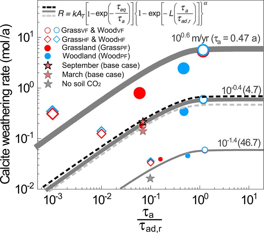
58                                                                                H. Wen et al.: Deepening roots can enhance carbonate weathering

Table 1. Key reactions and kinetic and thermodynamic parameters.

       Reaction                                                                                       log10 Keq             Standard                log10 k           Specific
                                                                                                      at 25 ◦ Ca            enthalpy            (mol/m2 /s)       surface area
                                                                                                                          ◦
                                                                                                                       (1H , kJ/mol)             at 25 ◦ Cd           (m2 /g)d
       Soil CO2 production through CO2 (g∗ ) and dissolving into CO2 (aq)
       (0) CO2 (g∗ ) ↔ CO2 (g)                                                                                   –                        –           −9.00                   1.0
       (1) CO2 (g)↔ CO2 (aq)                                                                             −1.46b                  −19.98                     –                    –
       (2) CO2 (aq) + H2 O ↔ H+ + HCO−
                                     3                                                                     −6.35                     9.10                   –                    –
                −     +      2−
       (3) HCO3 ↔ H + CO3                                                                                −10.33                     14.90                   –                    –
       Chemical weathering
       (4) CaCO3 (s) + CO2 (aq) + H2 O ↔ Ca2+ + 2HCO−
                                                    3                                                    −5.12c                  −15.41               −6.69                 0.84
                                                                                                         −4.52c
       (5)e CaAl2 Si2 O8 (s) + 8H+ ↔ Ca2+ + 2Al3+ + 2H4 SiO4 (aq)                                           26.58                         –         −11.00                 0.045
       (6)e KAlSi3 O8 (s) + 4H+ + 4H2 O↔ Al3+ + K+ + 3H4 SiO4 (aq)                                         −0.28                          –         −12.41                  0.20
       (7)e Al2 Si2 O5 (OH)4 (s) + 6H+ ↔ 2Al3+ + 2H4 SiO4 (aq) + H2 O                                        6.81                         –            12.97               17.50
     a Values of K were interpolated using the EQ3/6 database (Wolery et al., 1990), except Reactions (1) and (4) (i.e., K and K ). b CO (aq) concentrations were calculated
                  eq                                                                                                      1     4       2
     through CCO2 (aq) = K1 pCO2 . The prescribed CCO2 (aq) values were used as equilibrium constants in CrunchTope to describe how much soil CO2 was available for
     weathering. c Calcite in the upper soil (above horizon B) is mixed with other minerals and has small particle size (Macpherson and Sullivan, 2019b), is relatively impure,
     and therefore has a lower Keq value than those at depth with relatively pure calcite. The Keq of the impure calcite was calibrated by fitting field data of Ca and alkalinity.
     d The kinetic rate parameters and specific surface areas were from Palandri and Kharaka (2004), except Reaction (0). The kinetic rate constant of the source CO (g∗ )
                                                                                                                                                                         2
     dissolution (i.e., soil respiration rate constant, Reaction 0) was from Bengtson and Bengtsson (2007), Ahrens et al. (2015), and Carey et al. (2016); the specific surface area
                                                                          e
     was referred to that of soil organic carbon (Pennell et al., 1995). These reactions were only used in the base-case model as they occurred in upper soils in Konza. In the
     later numerical experiments, these reactions were not included so as to focus on carbonate weathering.

3     Reactive transport modeling                                                               and reproduced the observed soil pCO2 levels at a kinetic
                                                                                                rate constant of 10−9 mol/m2 /s (Reactions 0–1 in Table 1).
3.1      Base case: 1-D reactive transport model for the                                        This value is at the low end of the reported soil respira-
         Konza grassland                                                                        tion rates (10−9 –10−5 mol/m2 /s) (Bengtson and Bengtsson,
                                                                                                2007; Ahrens et al., 2015; Carey et al., 2016). The dissolution
A 1-D reactive transport model was developed using the                                          of CO2 (g) into CO2 (aq) follows Henry’s law CCO2 (aq) =
code CrunchTope (Steefel et al., 2015). The code solves                                         K1 pCO2 . Here K1 is the equilibrium constant of Reac-
mass conservation equations integrating advective and dif-                                      tion (1), which equals to Henry’s law constant. The extent of
fusive/dispersive transport and geochemical reactions. It has                                   CO2 (g) dissolution was constrained by CCO2 (aq) , which was
been extensively used in understanding mineral dissolution,                                     estimated using temperature-dependent K1 (following the
chemical weathering, and biogeochemical reactions (e.g.,                                        van ’t Hoff equation in Eq. S1) and measured soil CO2 data
Lawrence et al., 2014; Wen et al., 2016; Deng et al., 2017).                                    at different horizons (Table 2). These CCO2 (aq) values were
In this study, the base case had a porosity of 0.48 and a depth                                 then linearly interpolated for individual grid blocks in the
of 366.0 cm at a resolution 1.0 cm. Soil temperature was as-                                    model. Finally, these prescribed CCO2 (aq) values were used
sumed to decrease linearly from 17 ◦ C at the land surface to                                   as the equilibrium constants of the coupled Reactions (0–1)
8 ◦ C at 366.0 cm, within typical ranges of field measurements                                  in the form of CO2 (g∗ ) ↔ CO2 (aq), such that the soil CO2
(Tsypin and Macpherson, 2012). Detailed setup of domain,                                        values at different depth were represented (Sect. 4.1). In the
soil mineralogy, initial condition, and precipitation chemistry                                 base case, the soil profile of CCO2 (aq) was updated monthly
are in the Supplement.                                                                          based on the monthly soil CO2 data (Table 2). More details
                                                                                                about the implementation in CrunchTope are included in the
3.1.1      Representation of soil CO2                                                           Supplement.

The model does not explicitly simulate soil respiration (mi-
crobial activities and root respiration) that produces soil CO2 .
Instead, it approximates these processes by having a CO2
source phase CO2 (g∗ ) that continuously releases CO2 (g)

Biogeosciences, 18, 55–75, 2021                                                                                               https://doi.org/10.5194/bg-18-55-2021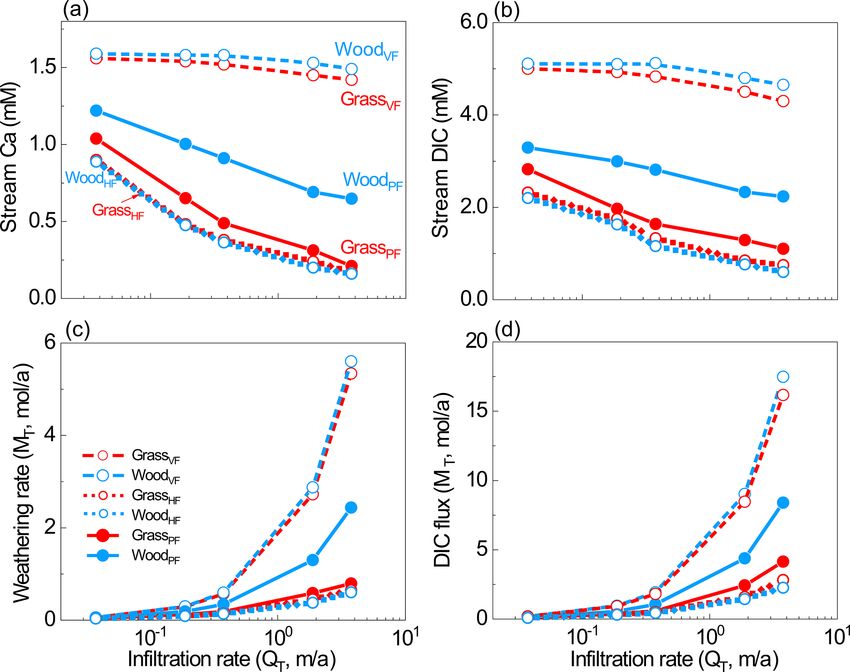
H. Wen et al.: Deepening roots can enhance carbonate weathering                                                                                                              59

Table 2. Measured CO2 (g) at different depths and corresponding estimated CCO2 (aq).

                              Time                                                           Soil depth                                                     Ways
                                                                                                                                                            obtaineda,b,c
   I. Grassland (Konza) cases
                                                        Horizon A                 Horizon AB                    Horizon B               Groundwater
                                                       (h = 16 cm)                    (84 cm)                    (152 cm)                  (366 cm)
   Soil T ◦ C                                                      17                         15                          13                          8     Estimated
   K1                                                   4.1 × 10⁻²                  4.4 × 10⁻²                 4.6 × 10⁻²                 5.4 × 10⁻²        Estimated
   1. Base case with monthly CO2 (g) (%) and CO2 (aq) (mol/L)
   CO2 (g) (%)                July                                3.6                         6.8                        6.6                        2.2     Measured
                              August                              1.4                         1.7                        7.2                        3.9     Measured
                              September                           0.6                         1.2                        3.9                        4.9     Measured
                              October                             0.5                         1.4                        2.5                        5.0     Measured
                              November                            0.6                         1.1                        2.2                        4.0     Measured
                              January                             0.3                         0.8                        1.1                        3.6     Measured
                              March                               0.2                         0.3                        0.5                        3.0     Measured
   CO2 (aq) (mol/L)           July                      1.5 × 10⁻³                  3.0 × 10⁻³                 3.0 × 10⁻³                 1.2 × 10⁻³        Estimated
                              August                    5.7 × 10⁻⁴                  7.5 × 10⁻⁴                 3.3 × 10⁻³                 2.1 × 10⁻³        Estimated
                              September                 2.5 × 10⁻⁴                  6.2 × 10⁻⁴                 1.8 × 10⁻³                 2.6 × 10⁻³        Estimated
                              October                   1.9 × 10⁻⁴                  6.2 × 10⁻⁴                 1.2 × 10⁻³                 2.7 × 10⁻³        Estimated
                              November                  2.5 × 10⁻⁴                  4.8 × 10⁻⁴                 1.0 × 10⁻³                 2.2 × 10⁻³        Estimated
                              January                   1.2 × 10⁻⁴                  3.5 × 10⁻⁴                 5.1 × 10⁻⁴                 1.9 × 10⁻³        Estimated
                              March                     8.2 × 10⁻⁵                  1.3 × 10⁻⁴                 2.3 × 10⁻⁴                 1.6 × 10⁻³        Estimated
   2. Numerical experiments with annual-average CO2 (g) (%) and CO2 (aq) (mol/L)
   CO2 (g)                    Annual                     1.0 ± 1.2                  1.9 ± 2.2                   3.4 ± 2.6                  3.8 ± 1.0        Measured
   CO2 (aq)                   Annual           (4.2 ± 5.0) × 10−4         (8.5 ± 9.7) × 10−4          (1.6 ± 1.2) × 10−3         (2.0 ± 0.5) × 10−3         Estimated
   II. Woodland cases (Calhoun site, South Carolina) numerical experiments with annual-average CO2 (g) (%) and CO2 (aq) (mol/L)
                                                       (h = 50 cm)                     (150 cm)                   (300 cm)                   (500 cm)
   Soil T ◦ C                                                  16                          13                         10                           8        Estimated
   K1                                                  4.2 × 10⁻²                 4.6 × 10⁻²                  4.9 × 10⁻²                 5.4 × 10⁻²         Estimated
   CO2 (g)                    Annual                     0.9 ± 0.1                  2.7 ± 0.6                   3.8 ± 0.6                  3.9 ± 0.7        Measured
   CO2 (aq)                   Annual           (4.5 ± 0.7) × 10−4         (1.3 ± 0.3) × 10−3          (1.9 ± 0.3) × 10−3         (1.9 ± 0.3) × 10−3         Estimated
a Monthly measured soil CO data for the Konza grassland (base case) were from Tsypin and Macpherson (2012); the soil CO in the grassland experiments was averaged from
                          2                                                                                            2
monthly measurements. More information on measurements at the Konza grassland is detailed in the Supplement. The annual-average soil CO2 in the woodland experiments was
from the forested Calhoun site in South Carolina (Billings et al., 2018). b CO2 (aq) values were estimated using Henry’s law: CCO2 (aq) = K1 pCO2 ; the temperature-dependent K1
was calculated following Eq. (S1). The CCO2 (aq) values at different soil depths were used to prescribe the available soil CO2 for chemical weathering. c Soil temperature was
estimated from the soil water and shallow groundwater temperature (Tsypin and Macpherson, 2012; Billings et al., 2018).

3.1.2     Reactions                                                                        duce field data. The kinetics follows the transition state the-

                                                                                           ory (TST) rate law (Plummer et al., 1978) r = kA 1 − IAP  Keq ,
In the model, the upper soil layers have more anorthite                                    where k is the kinetic rate constant (mol/m2 /s), A is the min-
(CaAl2 Si2 O8 (s)) and K-feldspar (KAlSi3 O8 (s)), and the                                 eral surface area per unit volume (m2 /m3 ), IAP is the ion
deeper subsurface contains more calcite (Table S1). The cal-                               activity product, and Keq is the equilibrium constant. The
cite volume increases from 0 % in the upper soil layer to 10 %                             term IAP / Keq quantifies the extent of disequilibrium: values
in the deep subsurface. Table 1 summarizes reactions and                                   close to 0 suggest far from equilibrium, whereas values close
thermodynamic and kinetic parameters. Soil CO2 increases                                   to 1.0 indicate close to equilibrium. At Konza, calcite in the
pore water acidity (Reactions 0–2) and accelerates mineral                                 upper soil (above horizon B) is mixed with other minerals,
dissolution (Reactions 3–6). Silicate dissolution leads to the                             has small particle size, and is considered impure (Macpher-
precipitation of clay (represented by kaolinite in Reaction 7).                            son and Sullivan, 2019a) and therefore has a lower Keq value
These reactions were included in the base case to repro-                                   than those at depth with relatively pure calcite. The Keq of

https://doi.org/10.5194/bg-18-55-2021                                                                                             Biogeosciences, 18, 55–75, 2021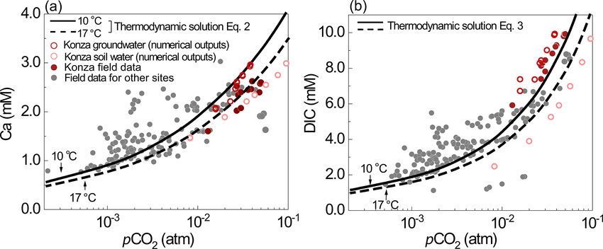
60                                                         H. Wen et al.: Deepening roots can enhance carbonate weathering

impure calcite (K4 ) was calibrated by fitting field data of Ca     macropores induced by dense, lateral-spread of roots mostly
and alkalinity. To reproduce the observed soil CO2 profile,         at depths less than 0.8 m (Jackson et al., 1996; Frank et al.,
the soil CO2 production rate (mol/m2 /a) at the domain scale        2010). These characteristics promote lateral flow (QL ) at the
(calculated by the mass change in the solid phase CO2 (g∗ )         shallow subsurface (Fig. 1a). At Konza, over 90 % of grass
over time) was assumed to increase with infiltration rates          roots were at the top 0.5 m, leading to high hydrologic con-
(Fig. S2). This is consistent with field observations that soil     ductivity in top soils (Nippert et al., 2012). In the woodland, a
CO2 production rate and efflux may increase with rainfall in        greater proportion of deep roots enhances vertical macropore
grassland and forest ecosystems (Harper et al., 2005; Patrick       development (Canadell et al., 1996; Nardini et al., 2016), re-
et al., 2007; Wu et al., 2011; Vargas et al., 2012; Jiang et al.,   duces permeability contrasts at different depths (Vergani and
2013). For example, Zhou et al. (2009) documented soil CO2          Graf, 2016), and is thought to facilitate more vertical water
production rates increasing from 3.2 to 63.0 mol/m2 /a when         flow to the depth (QG ). At the Calhoun site, over 50 % of
the annual precipitation increased from 400 to 1200 mm. Wu          roots are in the top 0.5 m in woodlands, with the rest pene-
et al. (2011) showed that increasing precipitation from 5 to        trating deeper (Jackson et al., 1996; Eberbach, 2003; Billings
2148 mm enhanced soil respiration by 40 % and that a global         et al., 2018).
increase of 2 mm precipitation per decade may lead to an in-           The experiments aimed to compare the general, averaged
crease of 3.8 mol/m2 /a for soil CO2 production. The simu-          behaviors rather than event-scale dynamics so the annual-
lated soil CO2 production rates across different infiltration       average soil CO2 data and corresponding prescribed CO2 (aq)
rates here (∼ 0.1–10 mol/m2 /a shown in Fig. S2) were close         concentrations were used (Table 2). The experiments fo-
to the reported belowground net primary production (be-             cused on calcite weathering (Reactions 0–4) and excluded
lowground NPP) of typical ecosystems: ∼ 0.8–100 mol/m2 /a           silicate weathering reactions (Reactions 5–7). The mineral-
for grasslands (Gill et al., 2002) and ∼ 0.4 –40 mol/m2 /a for      dissolution parameters from the base case were used for all
woodlands (Aragão et al., 2009).                                    experiments. We compared the relative significance of the
                                                                    hydrological (i.e., lateral versus vertical flow partitioning)
3.1.3    Flow partitioning                                          vs. respiratory (i.e., CO2 generation) influences of deepening
                                                                    roots. Though other potential differences might be induced
Rainwater enters soil columns at the annual infiltration            by deepening roots (e.g., water uptake, water table, and tran-
rate of 0.37 m/a, estimated based on the difference be-             spiration) (Li, 2019) and influence weathering, we assumed
tween measured precipitation (0.88 m/a) and evapotranspi-           they remain constant across the grassland and woodland
ration (0.51 m/a). At 50 cm, a lateral flow QL (soil water)         simulations to examine the relative influences of flow path
exited the soil column to the stream at 0.35 m/a. The rest          vs. CO2 generation on carbonate weathering.
recharged the deeper domain beyond 50 cm (to the ground-
water system) at 0.02 m/a (∼ 2 % of precipitation) and be-          3.2.1   Hydrological and biogeochemical differences in
came groundwater (Fig. 1a), a conservative value compared                   grasslands and woodlands
to 2 %–15 % reported in another study (Steward et al., 2011).
The groundwater flow QG eventually came out at 366.0 cm             Flow partitioning between lateral shallow flow and vertical
and was assumed to enter the stream as part of discharge            recharge flow is challenging to quantify and is subject to
(= QL + QG ). The flow field was implemented in Crunch-             large uncertainties under diverse climate, lithology, and land
Tope using the “PUMP” option.                                       cover conditions. The ratios of lateral flow in upper soils ver-
                                                                    sus the total flow inferred from a tracer study in a grassland
3.1.4    Calibration
                                                                    vary from ∼ 70 % to ∼ 95 % (Weiler and Naef, 2003). Har-
We used monthly alkalinity and Ca concentration data                man and Cosans (2019) found that the lateral flow rate at up-
(Sect. 2.2) for model calibration. The monthly Nash–                per soils over the overall infiltration can vary between 50 %
Sutcliffe efficiency (NSE) that quantified the residual vari-       and 95 %. Deeper roots in woodlands can increase deep soil
ance of modeling output compared to measurements was                permeability by over 1 order of magnitude (Vergani and Graf,
used for model performance evaluation (Moriasi et al., 2007).       2016). Assuming that the vertical, recharged flow water ul-
NSE values higher than 0.5 are considered acceptable.               timately leaves the watershed as baseflow, the ratio of the
                                                                    lateral versus vertical flow has been reported with a wide
3.2     Numerical experiments                                       range. In forests such as Shale Hills in Pennsylvania and Coal
                                                                    Creek in Colorado, ∼ 7 %–20 % of stream discharge is from
Numerical experiments were set up for grasslands and wood-          groundwater, presumably recharged by vertical flow (Li et
lands. The base case from Konza was used to represent grass-        al., 2017; Zhi et al., 2019). Values of QG / QT estimated
lands: data from the Calhoun site (the Calhoun Critical Zone        through base flow separation vary from 20 % to 90 % in
Observatory in South Carolina, USA) were used as repre-             forest/wood-dominated watersheds (Price, 2011), often neg-
sentative for woody sites (Billings et al., 2018). Grasslands       atively correlating with the proportion of grasslands (Mazvi-
are typically characterized by a high proportion of horizontal      mavi et al., 2004).

Biogeosciences, 18, 55–75, 2021                                                           https://doi.org/10.5194/bg-18-55-2021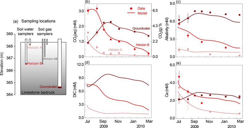
H. Wen et al.: Deepening roots can enhance carbonate weathering                                                                      61

Table 3. Physical and geochemical characteristics in numerical experiments.

   Soil respiration rates can vary between 10−9 and                    upper soils. Below the rooting depth, CO2 (g∗ ) was assumed
10−5 mol/m2 /s   in both grasslands and woodlands (Bengtson            to be smaller (by 10 times) to represent the potential soil CO2
and Bengtsson, 2007; Ahrens et al., 2015; Carey et al., 2016).         sources from microbial activities (Billings et al., 2018).
Soil CO2 levels may vary by 2–3 orders of magnitude de-                   Scenario 1 considered flow partitioning (Table 3). With the
pending on vegetation type and climate conditions (Neff and            large permeability contrast of soil and bedrock (over 4 orders
Hooper, 2002; Breecker et al., 2010). Soil CO2 levels are fur-         of magnitude) in Konza (Macpherson, 1996), the GrassPF
ther complicated by their dependence on topographic posi-              case (with QL = 95 % × QT and QG = 5 % × QT ) repre-
tion, soil depth, and soil moisture, all of which determine the        sents an end-member case for the grassland. The woodland
magnitude of microbial and root activities and CO2 diffusion           (WoodPF ) case was set to have 60 % lateral flow and 40 %
(Hasenmueller et al., 2015; Billings et al., 2018). There is           vertical flow into the deeper subsurface. This groundwater
however no consistent evidence suggesting which land cover             percentage is at the high end of flow partitioning and serves
exhibits higher soil respiration rate or soil CO2 level. Below         as an end-member case for woodlands (Vergani and Graf,
we describe details of the numerical experiments (Table 3)             2016). Scenarios 2 and 3 had no flow partitioning. Scenario
exploring the influence of hydrological versus biogeochemi-            2 had two cases with 100 % vertical flow via the bottom out-
cal impacts of roots.                                                  let (VF; WoodVF and GrassVF ); Scenario 3 had two cases
                                                                       with 100 % horizontal flow (HF; WoodHF and GrassHF ) via
3.3   Three numerical scenarios                                        the shallow outlet at 50 cm. These cases represent the end-
                                                                       member flow cases with 100 % lateral flow or 100 % vertical
Each scenario in Table 3 includes a grassland and woodland             flow. In addition, because the two cases have the same flow
case, with their respective profiles of calcite distribution and       scheme, they enable the differentiation of effects of soil CO2
soil pCO2 kept the same (columns 3 and 4 in Table 3). The              distribution versus hydrology differences. All scenarios were
only difference in different scenarios is the flow partition-          run under infiltration rates from 3.7 × 10⁻² to 3.7 m/a (10−4 –
ing (column 5). Soil pCO2 in the grassland (red line in col-           10−2 m/d), the observed daily variation range at Konza. This
umn 4) was set to reflect the annual average of the Konza              was to explore the role of flow regimes and identify condi-
site. Soil pCO2 (blue line) in the woodland was set to re-             tions where the most and least significant differences occur.
flect the annual average from the forest-dominant Calhoun                 Each case was run until steady state, when concentra-
site (Billings et al., 2018). In all scenarios, we assumed that        tions at the domain outlet became constant (within ± 5 %)
grasslands and woodlands had the same total CO2 (g∗ ) pro-             over time. The time to reach steady state varied from 0.1 to
ducing CO2 gas and CO2 (aq) but differed in depth distri-              30 a, depending on infiltration rates. The lateral flux (soil wa-
butions. The CO2 (g∗ ) depth distribution was constrained by           ter, ML = QL × CL ) and vertical fluxes (groundwater, MG =
CO2 (g) field data (Table 2). The distribution of CO2 (g∗ ) in         QG × CG ) were calculated at 50 and 366 cm, in addition to
grasslands is slightly steeper than that in the woodland, with         total fluxes (weathering rates, MT ). These fluxes multiplied
higher density of roots and more abundant CO2 (g∗ ) in the

https://doi.org/10.5194/bg-18-55-2021                                                               Biogeosciences, 18, 55–75, 2021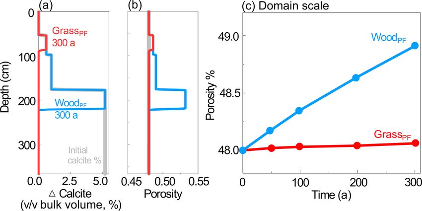
62                                                            H. Wen et al.: Deepening roots can enhance carbonate weathering

Figure 2. (a) Schematic representation of sampling depths in the Konza grassland; corresponding monthly dynamics of (b) CO2 (aq) and
CO2 (g), (c) alkalinity, (d) DIC, and (e) Ca concentrations. Lines represent modeling outputs at the corresponding sampling depth of monthly
field measurements (dots), including soil water at horizons A (16 cm) and B (152 cm), as well as groundwater (366 cm). The lines of CO2 (aq)
and CO2 (g) in panel (b) overlapped. Note that there are no DIC data so no dots in panel (d). The temporal trends of alkalinity, DIC, and Ca
mirrored those of soil CO2 , indicating its predominant control on weathering.

with unit cross-section area (m2 ) convert into rates in units          teristic timescale of mineral dissolution to reach equilib-
of moles per year (mol/a).                                              rium in a well-mixed system. The residence time τa , i.e., the
                                                                        timescale of advection, quantifies the overall water contact
3.4   Carbonate weathering over century timescales: soil                time with the whole domain. It was calculated by the product
      property evolution                                                of domain length (L) and porosity divided by the overall in-
                                                                                                      Lφ
                                                                        filtration rate (QT ): τa = Q  T
                                                                                                         . The reactive transport time τad,r
To compare the propagation of weathering fronts over longer             quantifies the water contact time with calcite as influenced by
timescales, we carried out two 300-year simulations for Sce-            both advection and diffusion/dispersion. The upscaled rate
nario 1 with flow partitioning under the base-case infiltra-            law is as follows:
tion rate of 0.37 m/a (i.e., GrassPF and WoodPF in Table 3).
During this long-term simulation, we updated calcite vol-                                                     τeq
                                                                        Rcalcite = kcalcite AT 1 − exp −
ume, porosity, and permeability. The calcite volume changes                                                   τa
were updated in each time step based on corresponding mass                                        α
                                                                                                τa
changes, which were used to update porosity. Permeabil-                  × 1 − exp −L                                .                  (1)
                                                                                               τad,r
ity changes were updated based on changes in local poros-
                                                           3
ity following the Kozeny–Carman equation: κκi,0i = ∅∅i,0i ×             Here k is the intrinsic rate constant measured for a min-
                                                                        eral in a well-mixed reactor, AT is the total surface area, L
  1−∅i,0 2

   1−∅i     (Kozeny, 1927; Costa, 2006), where κi and ∅i are            is domain length, α is geostatistical characteristics of spa-
permeability and porosity in grid i at time t, and κi,0 and ∅i,0        tial heterogeneity, and ττad,r
                                                                                                    a
                                                                                                        is the reactive time ratio quan-
are the initial permeability and porosity, respectively.                tifying the relative magnitude of the water contact time
                                                                        with the whole domain versus the contact time with the
3.5   Quantification of weathering rates and their                      reacting mineral. This rate law consists of two parts: the
      dependence on CO2 –carbonate contact                              effective dissolution
                                                                                        h       rates
                                                                                                   in i   homogeneous media repre-
                                                                                                       τeq
                                                                        sented by kAT 1 − exp − τa            and the heterogeneity fac-
To quantify the overall weathering rates and CO2 –carbonate                  n        h         ioα
contact in each scenario, we used the framework from a                  tor 1 − exp −L ττad,r a
                                                                                                         that quantifies effects of pref-
previously developed upscaled rate law for dissolution of               erential flow paths arising from heterogeneous distribution
spatially heterogeneously distributed minerals (Wen and Li,             of minerals. When ττad,r
                                                                                              a
                                                                                                 > 1, the water contact time with cal-
2018). The rate law says that three characteristic times are            cite zone is small, meaning the water is replenished quickly
important. The equilibrium time τeq represents the charac-              compared to the whole domain, leading to higher CO2 –

Biogeosciences, 18, 55–75, 2021                                                                https://doi.org/10.5194/bg-18-55-2021
H. Wen et al.: Deepening roots can enhance carbonate weathering 63
Figure 3. Simulated depth profiles of (A) calcite (vol %) and (B) soil CO2 production rate; (C) CO2 (g) (%), (D) DIC, and (E) Ca at 0.37 m/a;
and (F) effluent Ca concentrations at different infiltration rates. From top to bottom rows are Scenario 1 (GrassPF and WoodPF , with flow
partitioning, first row), Scenario 2 (GrassVF and WoodVF , with 100 % vertical flow, second row), and Scenario 3 (GrassHF and WoodHF , with
100 % lateral flow, last row). Red and blue colors present grassland and woodland, respectively. Lines and empty circles represent modeling
outputs, while filled circles with error bar in C are the annual-average CO2 (g) data (in Table 2). Arrows in A indicate flow conditions. In
F, soil water and groundwater refer to concentrations at the lateral (50 cm) and vertical (366 cm) outlets, respectively. Higher fractions of
vertical flow in WoodPF led to higher stream Ca concentration compared to GrassPF . In Scenario 2 and 3 without flow partitioning, stream
Ca concentrations were similar. The concentrations of DIC versus discharge are very similar to the Ca concentrations in F.
carbonate interactions. In contrast, a small ττad,r
a
ratio (< 1) 4 Results
reflects that water is replenished slowly in the reactive cal-
cite zones, leading to less CO2 –carbonate contact. These dif- 4.1 The thermodynamics of carbonate dissolution:
ferent timescales were calculated for Scenario 1–3 based on grassland at Konza as the base-case scenario
the flow characteristics and dissolution thermodynamics and
kinetics, as detailed in the Supplement. Values of τeq , τa , and The calibrated model reproduced the temporal dynamics
τad,r for all experiments are listed in Table S2. Note that nu- with a Nash–Sutcliffe efficiency (NSE) value > 0.6 and was
merical experiments in Scenario 1–3 focused on the short- considered satisfactory (Fig. 2). Note that the y axis is in-
term scale, with negligible changes in the solid phase. verted to display upper soils at the top and deep soils at the
bottom to be consistent with their subsurface position shown
in Fig. 2a. The measured CO2 (g) varied between 0.24 % and
https://doi.org/10.5194/bg-18-55-2021 Biogeosciences, 18, 55–75, 202164 H. Wen et al.: Deepening roots can enhance carbonate weathering
7.30 % (Fig. 2b right axis), 1 to 2 orders of magnitude higher higher at depths over 60 cm. The transition occurred between
than the atmospheric level of 0.04 %. The estimated CO2 (aq) 35 and 60 cm in the vicinity of the calcite–no-calcite inter-
(Fig. 2b left axis) generally increased with depth except in face at 55 cm, where concentrations of Ca and DIC increased
July and August when horizon B was at peak concentration. abruptly until reaching equilibrium. This thin transition was
The timing of the peaks and valleys varied in different hori- driven by fast calcite dissolution and rapid approach to equi-
zons. The CO2 (aq) reached maxima in summer in soil hori- librium, resulting in a short equilibrium distance. The equi-
zons A and B and decreased to less than 0.5 mM in winter librated DIC and Ca concentrations below 60 cm followed
and spring. The groundwater CO2 (aq) exhibited a delayed the similar increasing trend of CO2 (g) with depth in the deep
peak in September and October and dampened seasonal vari- zone (Fig. 3C1–E1).
ation compared to the soil horizons. The temporal trends of Figure 3F1 shows that Ca concentrations in soil water
alkalinity, DIC, and Ca in groundwater mirrored those of (light color) were lower than groundwater (dark color) and
soil CO2 at their corresponding depths, indicating the pre- varied with infiltration rates. The difference between soil wa-
dominate control of soil CO2 on carbonate weathering. The ter and groundwater Ca concentrations was relatively small
groundwater concentrations of these species were also higher at low infiltration rates because both reached equilibrium but
than soil concentrations. The simulated groundwater DIC diverged at high infiltration rates. Higher infiltration rates
(approximately summation of CO2 (aq) and alkalinity) was diluted soil water but not as much for groundwater. As ex-
> 6 times higher than that in upper soil (∼ 1.0 mM). The dis- pected, concentrations in the stream water, a mixture of soil
solved mineral volume was negligible for the simulation pe- water and groundwater (solid line), were in between these
riod (< 0.5 % v/v). Sensitivity analysis revealed that changes values but closely resembled soil water in the grassland. In
in flow velocities influenced concentrations in horizon A both cases, stream concentration decreased as infiltration in-
where anorthite is the dominating dissolving mineral (0– creased, indicating a dilution concentration–discharge rela-
1.8 m); their effects are negligible in horizon B and ground- tionship.
water where fast-dissolving calcite rapidly approaches equi- Scenario 2–3 for biogeochemical effects (without flow par-
librium. titioning). Scenarios 2 and 3 were end-member cases that
Several measurements/parameters were important in re- bracketed the range of rooting effects. Calcite and soil CO2
producing data. These include soil CO2 , which determined were distributed the same way as their corresponding flow
the CO2 (aq) level and its spatial variation, and equilibrium partitioning (PF) cases (Table 3). The WoodVF and GrassVF
constant (Keq ) of calcite dissolution. Imposition of monthly cases had 100 % flow going downward via the deeper cal-
variations and depth distributions of soil CO2 were essential cite zone maximizing the CO2 –water–calcite contact. In
to capture the variation of alkalinity and Ca data at different the WoodHF and GrassHF cases (Table 3), all water exited
horizons. The imposition of calcite Keq was also critical for at 50 cm, bypassing the deeper calcite-abundant zone and
reproducing Ca concentrations. Impurities were suggested to minimizing the CO2 –water–calcite contact. Figure 3A2–F2
affect Keq of natural calcite by a factor of ∼ 2.0 (Macpherson and 3A3–F3 show the VF (WoodVF and GrassVF ) and HF
and Sullivan, 2019a). Calcite Keq in upper soils had to be re- (WoodHF and GrassHF ) cases, respectively. Similar to the
duced by a factor of 3.8 in the model to reproduce concentra- flow partitioning cases, the concentrations of reaction prod-
tions in horizon A. The alkalinity and Ca concentrations were ucts were low in the shallow zone and increased over 10
not sensitive to kinetic parameters nor precipitation, because times within a short distance ∼ 5 cm at the depth of ∼ 50 cm.
carbonate dissolution rapidly approaches equilibrium. The woodland cases increased slightly more than the grass-
land cases because of the slightly steeper soil CO2 distribu-
4.2 Numerical experiments: the significance of tion (Fig. 3C2 and 3C3). Figure 3F2 indicates that the efflu-
hydrological flow partitioning ent Ca concentrations were slightly higher in WoodVF due to
the high soil CO2 level at the bottom outlet. The GrassHF and
Scenario 1 for hydro-biogeochemical effects with flow par- WoodHF case almost had the same effluent Ca concentrations
titioning (WoodP F and GrassP F ). Figures 3A1–E1 show at the upper soil (Fig. 3F3).
depth profiles of calcite and soil CO2 production rates and Concentration–discharge relationship and weathering
steady-state concentrations of reaction products. The soil rates in all cases. The VF cases had the highest effluent con-
CO2 production rate was highest in the upper soil at around centrations and weathering rates, whereas the HF cases had
10−6.5 mol/s and decreased to ∼ 10−9.5 mol/s at 366 cm lowest concentrations and weathering rates, and the GrassPF
(Fig. 3B1), consistent with the decline with soil depth ob- and WoodPF cases fell in between (Fig. 4a, b). This is be-
served in natural systems. The CO2 (g) level (released from cause the VF cases maximized the CO2 –calcite contact with
CO2 (g∗ )) increased with depth due to lower efflux into the 100 % flow through the calcite zone, whereas the HF cases
atmosphere in deeper zone and downward fluxes of CO2 – had minimum CO2 –calcite contact with most water bypass-
charge water from the upper soil (Fig. 3C1). Concentrations ing the calcite zone (column 3–4 in Table 3). The GrassPF and
of reaction products (Ca, DIC) were lower in the top 40 cm, WoodPF cases allowed different extent of contact prescribed
reflecting the lower carbonate-mineral background level, and by the amount of flow via the calcite zone. A case run with-
Biogeosciences, 18, 55–75, 2021 https://doi.org/10.5194/bg-18-55-2021H. Wen et al.: Deepening roots can enhance carbonate weathering 65
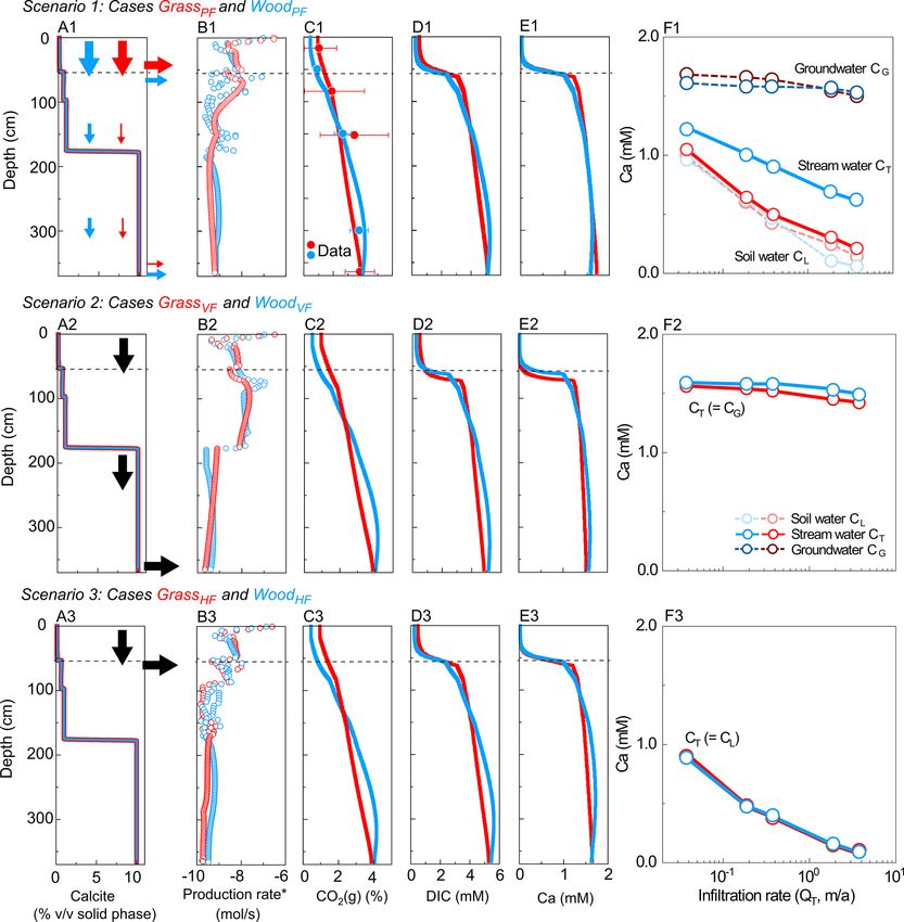
Figure 5. Predicted soil profiles of (a) calcite volume change (cal-
cite = initial calcite volume – current calcite volume) and (b) poros-
ity after 300 years; (c) predicted temporal evolution of domain-
scale porosity in the grassland and woodland. The infiltration rate is
0.37 m/a.
Figure 4. (a–b) Stream water Ca and DIC concentrations, and (c–
d) stream fluxes from all scenarios. Stream water was the overall for 300 years. More water flowing vertically through abun-
effluent from soil water and groundwater. The differences caused by dant calcite zones in WoodPF resulted in faster weathering
hydrological differences (VF, HF, and PF) were much larger than and a deeper reaction front at a depth of ∼ 210 cm compared
the differences within each pair with the same flow partitioning, to ∼ 95 cm in GrassPF (Fig. 5a). The depletion of calcite led
indicating significant hydrological impacts on weathering. to an increase in porosity (Fig. 5b), which was over 1 or-
der of magnitude higher at the domain scale of the woodland
than that in the grassland (Fig. 5c). Permeability evolution
out soil respiration (i.e., no CO2 (g∗ ), not shown) indicated had a similar trend to porosity (not shown here). This indi-
that Ca and DIC concentrations were more than an order of cates that if deeper roots promoted more water into deeper
magnitude lower than cases with soil respiration. In addition, soils, they would push reaction fronts deeper and control the
the PF and HF cases generally showed dilution patterns with position where chemically unweathered bedrock was trans-
concentration decreasing with infiltration rates, as compared formed into weathered bedrock. At timescales longer than
to the VF cases where a chemostatic pattern emerged with al- century scale, calcite may become depleted, which ultimately
most no changes as infiltration rates vary. This is because in reduces weathering rates (White and Brantley, 2003) and lead
the VF cases the concentrations mostly reached equilibrium to similar weathering fronts in grasslands and woodlands.
concentration. In the PF and HF cases, a large proportion of
water flows through soils with negligible calcite where the 4.3 The regulation of weathering rates by
water moves away from equilibrium as infiltration rates in- CO2 –carbonate contact time
crease.
Although weathering rates generally increased with infil- Natural systems are characterized by preferential flow paths
tration rates, the woodland increased more (4.6 × 10⁻² to such that flow distribution is not uniform in space. Weather-
2.4 mol/a in WoodPF ). The Ca fluxes in the VF cases (100 % ing in such systems with preferential flow in zones of differ-
vertical flow) were higher than flow partitioning cases be- ing reactivities has been shown to hinge on the contact time
cause they enabled maximum CO2 -charged water content between water and the reacting minerals instead of all miner-
with unweathered calcite at depth. Within each pair with als that are present (Wen and Li, 2018) (Eq. 1). Here we con-
the same flow pattern, the difference was mainly due to textualize the weathering rates in different scenarios (sym-
the distribution of soil CO2 . The difference in weathering bols) with predictions from an upscaled rate law developed
fluxes was 1 %–12 % and 1 %–5 % between HF cases and VF by Wen and Li (2018) that incorporates the effects of hetero-
cases, respectively, much smaller than differences between geneities in flow paths (Fig. 6). The time ratio ττad,r
a
compares
the PF cases. Comparing the HF and VF cases, differences in the domain water contact time (or residence time) with the
weathering fluxes were 73 % at 3.7 × 10⁻² m/a and 721 % at contact time with dissolving calcite. Note that τa is total do-
3.7 m/a, which is about 1–2 orders of magnitude higher than main pore volume VT /total water flow QT , and τad,r is total
differences induced by soil CO2 distribution. Between the reactive pore volume Vr /total water fluxes passing through
GrassPF and WoodPF cases, the differences were in the range reactive zone Qr . Also note that water passing through the re-
of 17 %–207 % at the flow range of 3.7 × 10⁻² –3.7 m/a. The active zone stays in the subsurface longer, such that it is older
DIC fluxes showed similar trends. water in general. The ratio ττad,r
a
is therefore akin to the frac-
Development of reaction fronts at the century scale. To ex- tion of older water compared to the total water fraction. The
plore the longer-term effects, we ran the PF cases at 0.37 m/a older water fraction Fow is the counterpart of the young wa-
https://doi.org/10.5194/bg-18-55-2021 Biogeosciences, 18, 55–75, 202166 H. Wen et al.: Deepening roots can enhance carbonate weathering
partitioning has a larger influence. At τa of 0.47 years, the
weathering rates in the VF cases were more than an order of
magnitude higher than those in the PF cases. The weathering
rate in the woodland was over 7 times that of the grassland.
In contrast, at τa of 47 years, the rate differences between
grass and woody cases were less than 25 %, largely because
the dissolution has reached equilibrium. In the VF and HF
cases where flow conditions were the same, the soil CO2 dis-
tribution in grassland and woodland differed only slightly,
leading to similar values of ττad,r
a
and weathering rates and
indicating minimal impacts of soil CO2 distribution. These
rates from numerical experiments closely follow the predic-
tion from the upscaled reaction rate law (gray lines, Eq. 1).
The rate law predicted that weathering rates increased from
HF cases with small ττad,r
a
values to VF cases where ττad,r
a
ap-
proached 1. It also showed that weathering rates reached their
maxima when all water flows through the reactive zone, i.e.,
when the fraction of older, reactive water is essentially 1.0.
Figure 6. Calcite weathering rate as a function of the reactive time
ratio ττad,r
a , a proxy of the fraction of the older, reactive water com-
pared to the total water fluxes. Symbols are rates from numerical 5 Discussion
experiments. Gray lines are predictions from the rate law equation
at α = 0.8 (Wen and Li, 2018). Large to small dots and thick to Because carbonate dissolution is thermodynamically con-
thin lines are for infiltration rates from 100.6 to 10−1.4 m/a. The trolled and transport limited, the overall weathering rates de-
red filled stars represent the monthly rates in September (highest pend on how much CO2 -charged water flushes through the
soil CO2 ) and March (lowest soil CO2 ) in the base case at 10−0.4 carbonate zone. This work indicates that deepening roots po-
(0.37) m/a; the black to gray dashed lines represent predictions with tentially enhance weathering rates in two ways. First, roots
increasing soil CO2 level (i.e., larger τeq ) from Eq. (1). The gray
can control thermodynamic limits of carbonate dissolution
filled star is for the case without soil CO2 . At any specific infiltra-
tion rate or τa , the VF and HF cases bracket the two ends, whereas
by regulating how much CO2 is transported downward and
the PF cases fall in between. The WoodPF case with deeper roots enters the carbonate-rich zone. In fact, the base-case grass-
enhanced the CO2 –water–calcite contact (i.e., larger ττad,r a ratios), land data and model reveal that the concentrations of Ca
leading to higher calcite weathering rates compared to grasslands. and DIC are regulated by seasonal fluctuation of pCO2 and
The differences of weathering rates induced by different soil CO2 soil respiration. Second, roots can control how much wa-
level were relatively small compared to those hydrological changes ter fluxes through the carbonate zone and export reaction
induced by rooting depth. products at equilibrium such that more dissolution can occur.
The numerical experiments indicate that carbonate weather-
ing at depth hinges on the recharge rate of delivery of CO2 -
enriched water. Deepening roots in woodlands that channel
ter fraction Fyw discussed in the literature (Kirchner, 2016, more water into unweathered carbonate at depths can elevate
2019). In GrassVF and WoodVF (open circles) where all CO2 - weathering rates by more than an order of magnitude com-
charged water flew through the deeper calcite zones, CO2 – pared to grasslands. Below we elaborate and discuss these
calcite interactions reached maximum such that values of two messages.
τa
τad,r approached 1.0, meaning all water interacted with cal-
cite. Under this condition, weathering rates were the highest 5.1 The thermodynamics of carbonate weathering:
among all cases. In contrast, in WoodHF and GrassHF (open control of temperature and pCO2
diamonds) where all CO2 -charged water bypassed the deeper
calcite zone, ττad,r
a
can be 1–3 orders of magnitude lower, and The base-case data and simulation showed that calcite disso-
weathering rates were at their minima. The ττad,r
a
value in the lution reaches equilibrium rapidly and is thermodynamically
water partitioning cases (GrassPF and WoodPF , filled circles) controlled (Sect. 4.1), which is generally well known and
fell in between. At the same τa , the WoodPF case with deep- echoes observations from literature (Tsypin and Macpher-
ening roots promoted CO2 –water–calcite contact (i.e., larger son, 2012; Gaillardet et al., 2019). The extent of dissolution,
τa
τad,r ) and dissolved calcite at higher rates. or solubility indicated in Ca and DIC concentrations, is de-
The magnitude of the rate difference also depends on the termined by soil CO2 levels that in turn hinge on ecosystem
overall flow rates (or domain contact time τa ). At fast flow functioning and climate. In hot, dry summer, soil respiration
with small τa (large symbols and thick lines in Fig. 6), flow rates reach maxima in upper soil horizons and pCO2 peaks
Biogeosciences, 18, 55–75, 2021 https://doi.org/10.5194/bg-18-55-2021H. Wen et al.: Deepening roots can enhance carbonate weathering 67
Figure 7. (a) Ca and (b) DIC data from the literature (gray dots) and prediction lines of Eqs. (2)–(3) at 10 ◦ C (solid line) and 17 ◦ C (dashed
line). Measured spring water concentrations are from carbonate-dominant catchments in the literature: Abongwa and Atekwana (2015),
Lopez-Chicano et al. (2001), Moral et al. (2008), Huang et al. (2015), Ozkul et al. (2010), Dandurand et al. (1982), Calmels et al. (2014),
Kanduc et al. (2012), and Tsypin and Macpherson (2012).
(Fig. 2). In wet and cold winter, soil pCO2 plummets, leading 10 ◦ C, the mean annual temperature, confirming the thermo-
to much lower Ca and DIC concentrations. Based on Reac- dynamics control of carbonate dissolution by soil CO2 lev-
tions (0–4) (Table 1) and temperature dependence of equilib- els. The equation lines closely predicted Ca and DIC under
rium constants, the following equations can be derived (de- high-pCO2 and lower-pH conditions (< 8.0), because these
tailed derivation in the Supplement) for Ca and DIC concen- conditions ensure the validity of the assumption of negligi-
trations in carbonate-dominated landscapes: ble CO2− 3 in the derivation of the equations. The presence of
1 cations and anions other than Ca and DIC can complicate the
CCa = Kt,25 × ef (T ) × pCO2 3
(2) solution and can bring significant variations of DIC and Ca
1 concentrations under the same pCO2 conditions.
CDIC = 2 Kt,25 × ef (T ) × pCO2 3 + K1,25 × ef (T ) × pCO2
High temperature (T = 17 ◦ C) leads to lower DIC and
◦
1H1 1 1 Ca concentrations by about 10 % due to the lower calcite
wheref (T ) = − − (3) and CO2 solubility at higher T . Higher T also elevates
4R T 298.15
pCO2 by enhancing soil respiration. Various equations have
Here CCa and CDIC are concentrations of Ca and DIC been developed in literature to predict soil pCO2 based on
(mol/L); pCO2 is in units of atm; Kt,25 is the total equilib- climate and ecosystem functioning indicators such as net
aCa2+ a 2
HCO−
3 primary production (NPP) (Cerling, 1984; Goddéris et al.,
rium constant Kt (= pCO2 = K1 K4 ) of the combined
◦ 2010; Romero-Mujalli et al., 2019a). These equations can be
Reactions (1) and (4) at 25 ◦ C; 1Ht is the correspond- used together with Eqs. (2–3) for the estimation of Ca and
◦
ing standard enthalpy (−35.83 kJ/mol); K1,25 and 1H1 DIC concentrations in carbonate-derived waters. Gaillardet
(−19.98 kJ/mol) are the equilibrium constant and standard et al. (2019) showed that pCO2 can increase by 2 times with
enthalpy of Reaction (1) (in Table 1); R is the gas constant T increasing from 9 to 17 ◦ C, which can elevate DIC and
(= 8.314 × 10⁻³ kJ/K/mol). Equations (2) and (3) imply that Ca concentrations over 50 %. Macpherson et al. (2008) ob-
DIC and Ca in upper soil water (0.2 m) are lower compared to served a 20 % increase in groundwater pCO2 in Konza over
groundwater (3.6 m) in the base case at Konza, due to lower a 15-year period and suggested that increased soil respiration
dissolved CO2 (aq) at higher temperature and higher diffusion under warmer climate may have elevated soil and groundwa-
rates in upper soil. ter pCO2 . Zhi et al. (2020) showed that the stream concen-
Equations (2) and (3) were tested with soil pCO2 and trations of dissolved organic carbon, a product of soil respi-
spring water chemistry data from eight carbonate-dominated ration, tripled in warmer years as minimum average temper-
catchments (Dandurand et al., 1982; Lopez-Chicano et al., ature approaches 0 ◦ C in a high elevation mountain. Hasen-
2001; Moral et al., 2008; Ozkul et al., 2010; Kanduc et al., mueller et al. (2015) demonstrated topographic controls on
2012; Calmels et al., 2014; Abongwa and Atekwana, 2015; soil CO2 . Soil CO2 and Ca and DIC concentrations are an
Huang et al., 2015) (also see the Supplement for details). integrated outcome of climate, soil respiration, subsurface
As shown in Fig. 7, spring water (representing groundwa- structures, and hydrological conditions.
ter) DIC and Ca concentrations increase with pCO2 . Equa-
tions (2)–(3) can describe these data and DIC and Ca levels
from numerical simulations from this work (empty dots in
Fig. 7). The lines of Eqs. (2)–(3) describe the relationship at
https://doi.org/10.5194/bg-18-55-2021 Biogeosciences, 18, 55–75, 2021You can also read