Towards kilometer-scale ocean-atmosphere-wave coupled forecast: a case study on a Mediterranean heavy precipitation event - Recent
←
→
Page content transcription
If your browser does not render page correctly, please read the page content below
Atmos. Chem. Phys., 21, 11857–11887, 2021
https://doi.org/10.5194/acp-21-11857-2021
© Author(s) 2021. This work is distributed under
the Creative Commons Attribution 4.0 License.

Towards kilometer-scale ocean–atmosphere–wave coupled forecast:
a case study on a Mediterranean heavy precipitation event
César Sauvage1,a , Cindy Lebeaupin Brossier1 , and Marie-Noëlle Bouin1,2
1 CNRM,    Université de Toulouse, Météo-France, CNRS, Toulouse, France
2 Laboratoire d’Océanographie Physique et Spatiale, Ifremer, University of Brest, CNRS, IRD, Brest, France
a now at: Physical Oceanography Department, Woods Hole Oceanographic Institution, Woods Hole, MA, USA

Correspondence: César Sauvage (sauvagecesar@hotmail.fr)

Received: 18 March 2021 – Discussion started: 26 March 2021
Revised: 2 July 2021 – Accepted: 2 July 2021 – Published: 9 August 2021

Abstract. The western Mediterranean Sea area is fre-               fordability to confidently progress towards operational cou-
quently affected in autumn by heavy precipitation events           pled forecasts.
(HPEs). These severe meteorological episodes, character-
ized by strong offshore low-level winds and heavy rain in
a short period of time, can lead to severe flooding and wave-
submersion events. This study aims to progress towards an          1   Introduction
integrated short-range forecast system via coupled model-
ing for a better representation of the processes at the air–       In the last decade, improving the forecast of intense weather
sea interface. In order to identify and quantify the coupling      events involving air–sea interactions has motivated oper-
impacts, coupled ocean–atmosphere–wave simulations were            ational forecast centers to develop and operate ocean–
performed for a HPE that occurred between 12 and 14 Oc-            atmosphere–wave coupled modeling platforms for short-
tober 2016 in the south of France. The experiment using            and medium-range weather predictions (see, for instance,
the coupled AROME-NEMO-WaveWatchIII system was no-                 the Geophysical Fluid Dynamics Laboratory (GFDL) model
tably compared to atmosphere-only, coupled atmosphere–             used at the National Weather Service, Bender et al., 2007, the
wave and ocean–atmosphere simulations. The results showed          Coupled Ocean/Atmosphere Mesoscale Prediction System
that the HPE fine-scale forecast is sensitive to both couplings:   for Tropical Cyclones (COAMPS-TC) operated at the Naval
the interactive coupling with the ocean leads to significant       Research Laboratory for hurricane prediction, Doyle et al.,
changes in the heat and moisture supply of the HPE that in-        2014, the global ocean–ice–atmosphere coupled prediction
tensify the convective systems, while coupling with a wave         system run at Environment and Climate Change Canada,
model mainly leads to changes in the low-level dynamics,           Smith et al., 2018, and the recent developments at the Eu-
affecting the location of the convergence that triggers con-       ropean Centre for Medium-Range Weather Forecasts, Mag-
vection over the sea.                                              nusson et al., 2019).
   Result analysis of this first case study with the AROME-           Tropical cyclones (TCs) above all have been known for
NEMO-WaveWatchIII system does not clearly show ma-                 long to be impacted by the surface cooling of the ocean they
jor changes in the forecasts with coupling and highlights          generate (e.g., Bender et al., 1993; Bender and Ginis, 2000;
some attention points to follow (ocean initialization notably).    Bao et al., 2000). Realistic simulations have shown that the
Nonetheless, it illustrates the higher realism and potential       initial state of the ocean, namely, the sea surface tempera-
benefits of kilometer-scale coupled numerical weather pre-         ture (SST) and stratification, may significantly reduce the TC
diction systems, in particular in the case of severe weather       intensity (e.g., Chan et al., 2001). Several large-scale stud-
events over the sea and/or in coastal areas, and shows their af-   ies have shown that using ocean–atmosphere coupling im-
                                                                   proves in a statistical way the prediction of TCs with respect
                                                                   to atmosphere-only simulations in every cyclonic basin (e.g.,

Published by Copernicus Publications on behalf of the European Geosciences Union.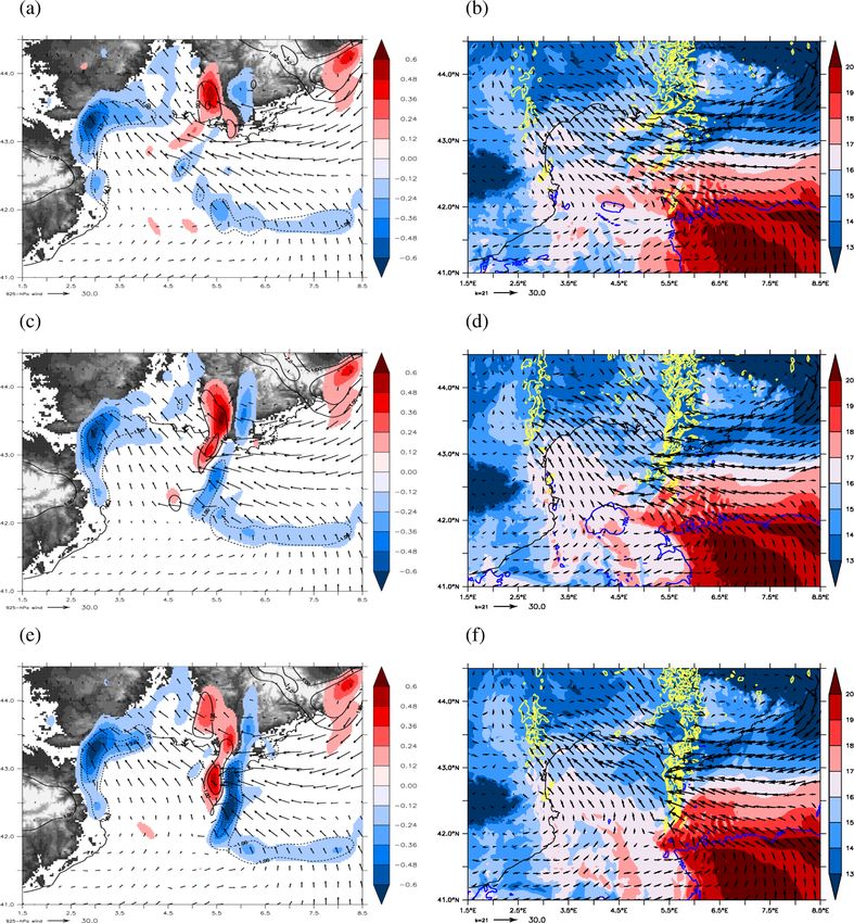
11858                                C. Sauvage et al.: Towards kilometer-scale ocean–atmosphere–wave coupled forecast

Bender et al., 2007; Samson et al., 2014; Mogensen et al.,         ing – Skamarock et al., 2008) and WAM (the ocean WAve
2017; Lengaigne et al., 2018). Using 3D ocean models in            Model – The Wamdi Group, 1988) models.
coupled configurations is mandatory to accurately represent           Generally related to cyclogenesis, the Mediterranean Sea
the complex subsurface processes (e.g., upwelling) respon-         is also prone to high and local wind of continental origin,
sible for the SST cooling (Yablonsky and Ginis, 2009). As          channelled and accelerated in the steep surrounding valleys,
TC development is known to be sensitive to both enthalpy           such as mistral or bora, which usually last several days and
and momentum transfer coefficients (Emanuel, 1986), tak-           generate very rough sea states and sometimes result in strong
ing into account the wave impact on the sea surface rough-         damages (e.g., Ardhuin et al., 2007). Several case studies in-
ness can also influence the TC representation in numerical         vestigated the impact of mistral or bora wind on the ocean
models. Case studies using ocean–atmosphere–wave coupled           and the impact of using ocean–atmosphere or atmosphere–
configurations showed an influence of wave growth on the           wave coupled models (e.g., Loglisci et al., 2004; Pullen et al.,
TC intensity and development (e.g., Olabarrieta et al., 2012;      2007; Small et al., 2012; Ricchi et al., 2016; Ličer et al.,
Lee and Chen, 2012; Doyle et al., 2014; Pianezze et al.,           2016; Seyfried et al., 2019). They showed a quick evolution
2018). Sensitivity tests using representation of the surface       of the SST and currents during this type of event, with a sig-
fluxes including the impact of sea spray showed more con-          nificant feedback on the surface heat and momentum fluxes
trasted results, depending on the parameterization used and        but no significant change in the low-level atmospheric flow.
on the case studied (e.g., Wang et al., 2001; Gall et al., 2008;      In the present study, we investigate the impact of ocean–
Green and Zhang, 2013; Zweers et al., 2015). Most of the           atmosphere–wave coupling on a different kind of Mediter-
coupled configurations used for improving the TC forecast          ranean extreme weather event, namely, a heavy precipitation
have horizontal resolutions of 10–25 km, enabling them to          event (HPE, Ducrocq et al., 2014, 2016). Such events gener-
cover large oceanic basins and fine enough to properly repre-      ally occur in autumn and are characterized by a large amount
sent relatively large-scale events like TCs. Only recent case      of precipitation over a small area in a very short time, caus-
studies make use of kilometric horizontal resolutions permit-      ing huge flash floods leading to considerable damages and
ting us to simulate more accurately the fine-scale processes       numerous casualties (e.g., Petrucci et al., 2019). These events
within the TC structure (e.g., Lee and Chen, 2012; Green and       are usually generated by quasi-stationary mesoscale convec-
Zhang, 2013; Pianezze et al., 2018).                               tive systems (MCSs) fed by strong offshore low-level winds
   Extreme events also often occur in the Mediterranean            over the warm Mediterranean Sea. Air–sea processes are thus
Sea. For instance, medicanes are severe storms looking like        key elements in the development of those HPEs (e.g., Duf-
TCs in their developed phase, although smaller in size and         fourg and Ducrocq, 2011). Rainaud et al. (2017), using the
weaker (e.g., Lionello et al., 2003; Renault et al., 2012;         coupling between the WMED (Western Mediterranean Sea)
Ricchi et al., 2017; Varlas et al., 2018, 2020; Bouin and          configurations of the AROME (Application of Research to
Lebeaupin Brossier, 2020b). In medicanes as in tropical cy-        Operations at MEsoscale – Seity et al., 2011; Fourrié et al.,
clones, ocean surface cooling is observed, primarily affect-       2015) atmosphere model at 2.5 km resolution and NEMO
ing the heat and moisture exchanges. Case studies based            at a 1/36◦ resolution (Lebeaupin Brossier et al., 2014), re-
on coupled simulations gave contrasting results on the im-         asserted the importance of an interactive ocean and its im-
pact of the feedback from the waves or the ocean on med-           pact on the surface evaporation water supply for HPEs. In
icanes. For instance, Ricchi et al. (2017) investigating the       addition to this, Thévenot et al. (2016), Bouin et al. (2017),
medicane of November 2011 using COAWST (Coupled                    and Sauvage et al. (2020) showed the importance of tak-
Ocean Atmosphere–Wave Sediment Transport, Warner et al.,           ing the sea state into account in the calculation of air–sea
2010) at 5 km resolution and Bouin and Lebeaupin Brossier          fluxes during Mediterranean HPEs, with a significant impact
(2020b) studying the one occurring in November 2014                on the location of the heavy precipitation. Indeed, the pa-
through high-resolution coupling (1.3 km for the atmosphere        rameterization of sea surface turbulent fluxes is key in repre-
using MESO-NH Mesoscale Non-Hydrostatic Model – Lac                senting the exchanges between the different compartments.
et al., 2018 and 1/36◦ for the ocean using NEMO Nucleus            Generally implemented as bulk parameterizations (e.g., Cou-
for European Modelling of the Ocean – Madec and the                pled Ocean–Atmosphere Response Experiment (COARE)
NEMO system team, 2008) showed that the direct impact              3.0, Fairall et al., 2003), several formulations enable us to
of the ocean coupling did not significantly change the track       represent the sea state impact on the momentum and heat
and intensity of the medicanes. Ricchi et al. (2017) suggested     fluxes (Oost et al., 2002; Taylor and Yelland, 2001; Sauvage
nevertheless that the way to calculate the sea surface rough-      et al., 2020).
ness, and more generally the air–sea processes, can affect            The studies listed above demonstrate the interest of more
significantly the results by notably playing on the intensifi-     complete regional simulating systems in better predicting
cation of the near-surface wind. Also, Varlas et al. (2020)        high-impact events involving air–sea interactions and com-
showed an overall improvement of the forecast skill over the       bining the capabilities of fine-scale (1 to 2 km in horizontal
sea using a two-way coupling between the atmosphere and            resolution) models with ocean–atmosphere–wave coupling.
waves, respectively, the WRF (Weather Research Forecast-           Also, the continuous increase in high-performance comput-

Atmos. Chem. Phys., 21, 11857–11887, 2021                                          https://doi.org/10.5194/acp-21-11857-2021
C. Sauvage et al.: Towards kilometer-scale ocean–atmosphere–wave coupled forecast                                            11859

Figure 1. The NEMO-AROME-WW3 coupled architecture and domains illustrated by orography (of the AROME-France domain in the
SURFEX “area”) and the NWMED72 bathymetry (in the NEMO box). The SURFEX-OASIS interface (red arrows) is detailed in Voldoire
et al. (2017), and the AROME-SURFEX links (green arrows) are described in Masson et al. (2013) and Seity et al. (2011). See text and
Table 1 for the exchanges involving NEMO and WW3.

ing capabilities fosters the development of such coupled            The details of the model configurations and the exchange
modeling systems with kilometric resolution and makes them          management are given in the following for clarity purposes.
usable for operational forecasting (e.g., Pullen et al., 2017;
Lewis et al., 2018, 2019a, b, c).                                   2.1     The component models
   In this context, the present study describes a new kilo-
metric regional coupled system involving the Météo-France           2.1.1    The atmospheric model
high-resolution operational numerical weather prediction
(NWP) model AROME-France, the WaveWatch III wave                    The non-hydrostatic AROME NWP model is used in this
model (hereafter WW3, Tolman, 1992) and the NEMO ocean              study, with the same forecast configuration as the one
model, which paves the way to the future coupled regional           operationally used at Météo-France in 2016 (AROME-
convection-resolving NWP system of Météo-France. This               France, cy41t1, Seity et al., 2011; Brousseau et al., 2016)
system will be used here to assess the coupling impacts dur-        with a 1.3 km horizontal resolution and a domain cen-
ing an HPE which occurred from 12 to 14 October 2016.               tered over France (Fig. 1), which notably covers the north-
   A detailed description of the coupled system is given in         western Mediterranean Sea. The AROME orography is ex-
Sect. 2. The main characteristics of the studied HPE and            tracted from the Global 30 Arc-Second Elevation Data Set
the numerical set-up are presented in Sect. 3. Then the             (GTOPO30) database (Gesch et al., 1999). The vertical grid
contribution of the two-way coupled atmosphere–wave and             has 90 hybrid η levels with a first-level thickness of almost
atmosphere–ocean is analyzed in Sect. 4. In Sect. 5 the re-         5 m. The time step is 50 s.
sults obtained using the ocean–atmosphere–wave system are              In AROME, the advection scheme is semi-Lagrangian,
discussed. Finally, conclusions are given in Sect. 6.               and the temporal scheme is semi-implicit. The 1.5-order tur-
                                                                    bulent kinetic energy scheme from Cuxart et al. (2000) is
                                                                    used. Due to its high resolution, the deep convection is ex-
2   The ocean–atmosphere–wave coupled system                        plicitly solved in AROME, whereas the shallow convection
                                                                    is solved with the eddy diffusivity Kain–Fritsch (EDKF, Kain
This section presents the tri-coupled system that combines          and Fritsch, 1990) parameterization. The ICE3 one-moment
the ocean–atmosphere coupling previously developed be-              microphysical scheme (Pinty and Jabouille, 1998) is used
tween AROME and NEMO by Rainaud et al. (2017) and the               to compute the evolution of five hydrometeor species (rain,
wave–atmosphere interactive exchanges with the AROME-               snow, graupel, cloud ice and cloud liquid water). Radiative
WW3 coupling as fully described by Sauvage et al. (2020).           fluxes are computed with the Fouquart and Bonnel (1980)

https://doi.org/10.5194/acp-21-11857-2021                                          Atmos. Chem. Phys., 21, 11857–11887, 2021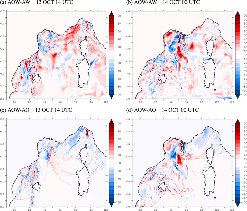
11860                                C. Sauvage et al.: Towards kilometer-scale ocean–atmosphere–wave coupled forecast

scheme for short-wave radiation and the RRTM (Rapid Ra-            from the Banque Hydro database (hydro.eaufrance.fr) and
diative Transfer Model, Mlawer et al., 1997) scheme for            in the monthly climatology of Ludwig et al. (2009) for the
long-wave radiation.                                               Ebro, Júcar and Tiber rivers temporally interpolated to give
   The surface exchanges are computed by the SURFace EX-           daily values. Each river inflow is injected in one grid point in
ternalisé (SURFEX) surface model (Masson et al., 2013)             the surface (as precipitation).
considering four different surface types: land, towns, sea and
inland waters (lakes and rivers). Output fluxes are weight-        2.1.3    The wave model
averaged inside each grid box according to the fraction of
each respective tile defined with physiographic data from the
                                                                   The wave model is WW3 (Tolman, 1992) in version 5.16
ECOCLIMAP database (Masson et al., 2003) before being
                                                                   (The WAVEWATCH III Development Group, 2016). The
provided to the atmospheric model at every time step. Ex-
                                                                   WW3 domain and bathymetry correspond to the NEMO-
changes over land are computed using the ISBA (Interac-
                                                                   NWMED72 grid (at a 1/72◦ horizontal resolution), as pre-
tions between Soil, Biosphere and Atmosphere) parameter-
                                                                   viously presented in Sauvage et al. (2020). The time step is
ization (Noilhan and Planton, 1989). The formulation from
                                                                   60 s.
Charnock (1955) is used for inland waters, whereas the Town
                                                                      The set of parameterizations from Ardhuin et al. (2010)
Energy Balance (TEB) scheme is activated over urban sur-
                                                                   is used, as for most of the wave forecasting centers (Ard-
faces (Masson, 2000). The treatment of the sea surface ex-
                                                                   huin et al., 2019). Thus, the swell dissipation is computed
changes in AROME-SURFEX is done here with the WASP
                                                                   with the Ardhuin et al. (2009) scheme, and the wind input
(Wave-Age-dependent Stress Parameterization) scheme, de-
                                                                   parameterization is from Janssen (1991). Nonlinear wave–
tailed in Sauvage et al. (2020) and below, and the albedo is
                                                                   wave interactions are computed using the discrete interaction
computed following the Taylor et al. (1996) scheme.
                                                                   approximation (Hasselmann et al., 1985). The parameteriza-
                                                                   tion of the reflection by shorelines is described in Ardhuin
2.1.2   The ocean model
                                                                   and Roland (2012). Moreover, the computation of the depth-
                                                                   induced breaking is based on the algorithm from Battjes and
The NWMED72 configuration of the NEMO ocean model
                                                                   Janssen (1978), and the bottom friction formulation follows
(version 3_6; Madec and the NEMO team, 2016) presented
                                                                   Ardhuin et al. (2003).
in (Sauvage et al., 2018) is used here. It covers the northwest-
ern Mediterranean basin (Fig. 1) with a 1/72◦ horizontal res-
olution (from 1 to 1.3 km resolution) and uses 50 stretched        2.2     Air–sea exchanges and coupling
z levels in the vertical, with a first-level thickness of 0.5 m.
This configuration has two open boundaries: a southern open        The coupled system AROME-NEMO-WW3 is implemented
boundary near 38◦ N south of the Balearic Islands and Sar-         using the SURFEX-OASIS coupling interface developed by
dinia and an eastern open boundary across the Tyrrhenian           Voldoire et al. (2017). This interface permits the field ex-
Sea (12.5◦ E).                                                     changes between the atmospheric and ocean models on the
   In NWMED72, the Total Variance Dissipation (TVD)                one hand and between the atmospheric and wave models on
scheme is used for tracer advection in order to conserve           the other hand (Fig. 1 and Table 1).
energy and enstrophy (Barnier et al., 2006). The vertical             NEMO provides to the OASIS3-MCT coupler (OASIS
diffusion follows the standard turbulent kinetic energy for-       hereafter, Craig et al., 2017) the mean SST and horizontal
mulation of NEMO (Blanke and Delecluse, 1993). In case             surface current components (us and vs ) at the coupling fre-
of unstable conditions, a higher diffusivity coefficient of        quency of 1 h. At the same coupling frequency, WW3 pro-
10 m2 s−1 is applied (Lazar et al., 1999). The sea surface         vides the peak period of the wind sea (Tp ) to OASIS. These
height is a prognostic variable solved thanks to the filtered      fields, after interpolation onto the AROME (SURFEX) grid,
free-surface scheme of Roullet and Madec (2000). A no-slip         are used to compute surface fluxes at each subsequent atmo-
lateral boundary condition is applied, and the bottom fric-        spheric time step. The wind components of the first atmo-
tion is parameterized by a quadratic function with a coeffi-       spheric level (ua , va ) and the air–sea fluxes at the interface –
cient depending on the 2D mean tidal energy (Lyard et al.,         namely, the solar heat flux Qsol , the non-solar heat flux Qns ,
2006; Beuvier et al., 2012). The diffusion is applied along        the two components of the horizontal wind stress τu and τv
isoneutral surfaces for the tracers using a Laplacian oper-        and the atmospheric freshwater flux EMP – are computed
ator with the horizontal eddy diffusivity value νh fixed at        by SURFEX and provided to OASIS, which then averages
15 m2 s−1 . For the dynamics (velocity), a bi-Laplacian oper-      them over 1 h and interpolates and sends them to WW3 (for
ator is used with the horizontal viscosity coefficient ηh fixed    ua and va ) or NEMO (for Qsol , Qnet , τu , τv , and EMP) at
at 1.108 m4 s−1 . The time step is 120 s.                          the coupling frequency. Detailed information on the different
   The runoff forcing consists of daily observations for 25        coupling namelists for each model is given in Appendix A.
French rivers around the northwestern Mediterranean Sea               The air–sea fluxes are computed taking into account near-
(see Sauvage et al., 2018, for the complete list) collected        surface atmospheric and oceanic parameters, following the

Atmos. Chem. Phys., 21, 11857–11887, 2021                                           https://doi.org/10.5194/acp-21-11857-2021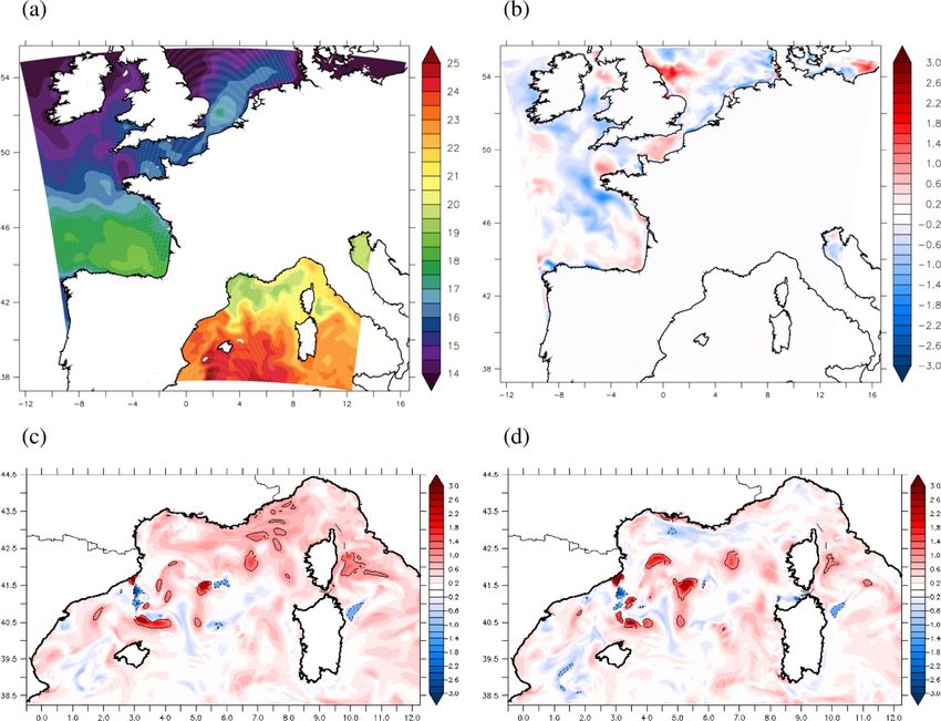
C. Sauvage et al.: Towards kilometer-scale ocean–atmosphere–wave coupled forecast                                               11861

Table 1. List of the exchanged fields.                                   The turbulent heat fluxes are also expressed as functions
                                                                      of the air–sea gradients:
    Source model to target model
                                                                      H = ρa cpa CH kU s − U a k1θ,
    Annotation     Field description
                                                                      LE = ρa Lv CE kU s − U a k1q,                                (5)
    NEMO to AROME/SURFEX
                                                                      with cpa the air heat capacity. 1θ and 1q represent the air–
    θs             Sea surface temperature                            sea gradients of potential temperature (θs − θa ) and specific
    us             Sea surface zonal current                          humidity (qs − qa ), respectively.
    vs             Sea surface meridional current
                                                                        Each transfer coefficient (CX ) can be expressed as
    AROME/SURFEX to NEMO                                                        1   1
                                                                      CX = cx2 cd2 ,                                               (6)
    τu             Zonal component of the wind stress
    τv             Meridional component of the wind stress            where X/x is D/d for wind stress, H / h for sensible heat
    Qns            Non-solar heat flux                                                                  1

    Qsol           Solar net heat flux                                and E/e for latent heat. The cx2 coefficients are a function
    EMP            Freshwater flux                                    of ψx (ζ ) that describes empirically the stability, ζ is the z/L
                                                                      ratio with L the Obukhov length, and z0 is the sea surface
    WW3 to AROME/SURFEX
                                                                      roughness length. Therefore,
    Tp             Wind–sea peak period                                                     1/2
    Hs             Significant wave height (not used in WASP)          1/2                 cxn
                                                                      cx (ζ ) =            1/2
                                                                                                                                   (7)
    AROME/SURFEX to WW3                                                             1 − cxn
                                                                                         κ ψx (ζ )
    ua             Zonal wind at first level                          and
    va             Meridional wind at first level                      1/2         κ
                                                                      cxn =               ,                                        (8)
                                                                               ln(z/z0x )
                                                                      with the subscript n referring to neutral (ζ = 0) stability, z to
radiative schemes (Fouquart and Bonnel, 1980; Mlawer
                                                                      the reference height and κ to von Karman’s constant. The
et al., 1997) and the WASP turbulent flux parameterization:
                                                                      sea surface roughness length z0 is defined by two terms,
Qsol = (1 − α)SWdown ,                                          (1)   Charnock’s relation (Charnock, 1955) and a viscous contri-
                                                                      bution (Beljaars, 1994):
Qns = LWdown − σ θs4 − H − LE,                                 (2)
                                                                             αch u2∗ 0.11ν
where SWdown and LWdown are the incoming components                   z0 =          +      ,                                       (9)
                                                                               g       u∗
of the solar and infrared radiations, respectively. θs is the
SST, α is the albedo,  is the emissivity and σ is the Stefan–        with ν the kinematic viscosity of dry air and the Charnock
Boltzman constant. Turbulent heat fluxes (H for sensible and          coefficient αch . In WASP, z0 depends on the wave age (χ)
LE for latent) are calculated with WASP (see the following)           through the Charnock coefficient (αch ), which is a power
and thus depend on the wind speed and on the air–sea gradi-           function of χ (αch = Aχ −B ; see Eq. (8) and Appendix A in
ents of temperature and humidity, respectively, and on trans-         Sauvage et al., 2020), and χ is defined as
fer coefficients CH and CE , respectively, which themselves                    gTp
depend on air stability and wave age (see the following).             χ=               ,                                          (10)
                                                                             2π kU a k
   The atmospheric freshwater flux is given by
                                                                      where g is the acceleration of gravity and Tp is the peak pe-
EMP = E − Pl − Ps ,                                             (3)   riod of waves corresponding to the wind sea, i.e., the waves
                                                                      generated by the local wind that are growing (χ < 0.8) or
where E is the evaporation, corresponding to E = LE/Lv
                                                                      in equilibrium with the wind (0.8 ≤ χ < 1.2) and that are
with Lv the vaporization heat constant. Pl and Ps are the liq-
                                                                      aligned with the local wind. The reader can refer to Sauvage
uid and solid surface precipitation rates (given by AROME).
                                                                      et al. (2020) for an enlarged description of WASP.
  The wind stress takes into account the ocean surface cur-
                                                                         The AROME-France domain is more extended than the
rent (given by NEMO), as follows:
                                                                      NWMED72 domain of NEMO and WW3, and as the At-
τ = (τu , τv ) = ρa CD kU s − U a k(U s − U a ) = ρu2∗ ,        (4)   lantic Ocean and the Adriatic Sea are not represented, there
                                                                      is no air–sea coupling in these areas: the SST comes from
with ρa the air density, U a = (ua , va ) the wind at the lowest      the AROME-France initial analysis and is constant during
atmospheric model level (around 5 m here), U s = (us , vs ) the       the run, horizontal current is considered null, and the peak
ocean surface current and u∗ the friction velocity. CD is the         period is computed inside WASP as a function of the wind
drag coefficient given by the turbulent flux parameterization.        speed (Tp = 0.5kU a k).

https://doi.org/10.5194/acp-21-11857-2021                                               Atmos. Chem. Phys., 21, 11857–11887, 2021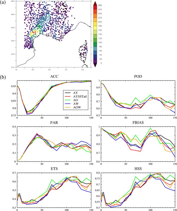
11862                                   C. Sauvage et al.: Towards kilometer-scale ocean–atmosphere–wave coupled forecast

Figure 2. Mean surface and atmospheric low-level conditions: (a, b) enthalpy flux over the sea (H +LE, colors, W m−2 ), convective available
potential energy (CAPE, green contours every 750 J kg−1 ) and 10 m wind (arrows, m s−1 ) and (c, d) θw ’ (colors, K) and wind (arrows, m s−1 )
at 925 hPa and total rainfall amounts (green contours every 50 mm) from the AW forecast during (a, c) the initiation phase (Phase I, between
13 October 2016 03:00 UTC and 18:00 UTC) and (b, d) the mature phase (Phase II, between 13 October 2016 19:00 UTC and 14 October
2016 03:00 UTC). See text and Sauvage et al. (2020) for more details. The dashed purple box in (a) indicates the Azur zone. The dashed
boxes in (c) indicate the Hérault (purple) and offshore (cyan) areas for precipitation analyses.

3     Evaluation                                                         ern Tunisia. The event is also marked by a strong easterly
                                                                         flow that originated from the southern Alps and intensified
3.1    Case study                                                        during the two first phases of the event (Fig. 2). This east-
                                                                         erly flow triggered large sea surface heat exchanges over the
The HPE studied here is described in detail in Sauvage et al.            Ligurian Sea and along the French Riviera (Fig. 2a, b) due
(2020). Its main characteristics are briefly given in the fol-           to strong wind (up to 20 m s−1 observed at the Azur buoy
lowing.                                                                  at 7.8◦ E −43.4◦ N) and to large air–sea gradients. These
   The synoptic situation of the event has been defined as               large fluxes gradually warmed and moistened the low-level
a “cyclonic southerly” kind (Nuissier et al., 2011), charac-             air mass along its path towards the Gulf of Lion. The Gulf of
terized by a slow moving trough extending from the British               Lion was initially affected by the rapid easterly flow, produc-
Isles to Spain that induced at upper level a southwesterly flow          ing a young sea with significant wave height (Hs ) up to 6 m
over southeastern France. At low level, a cyclonic circula-              and strong air–sea fluxes. As the system moved eastwards
tion established and induced a southeasterly flow across the             with the highest wind intensity, the sea state evolved in time
western Mediterranean Sea that originated from southeast-                from a well-developed sea to swell in this region. Throughout

Atmos. Chem. Phys., 21, 11857–11887, 2021                                                  https://doi.org/10.5194/acp-21-11857-2021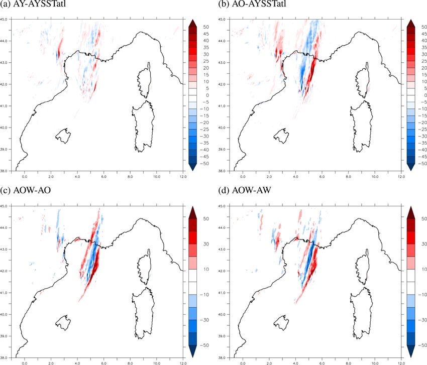
C. Sauvage et al.: Towards kilometer-scale ocean–atmosphere–wave coupled forecast 11863
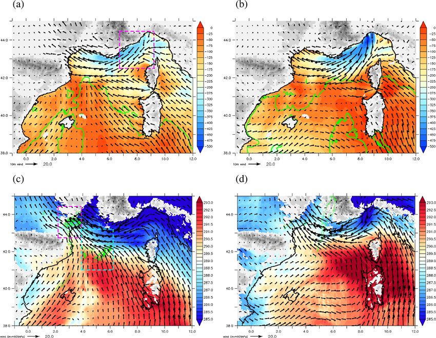
Figure 3. (a) SST (◦ C) forecast in AOW at 14:00 UTC on 13 October (forecast basis: 13 October 00:00 UTC) and (b) differences in initial
SST fields (◦ C, 13 October 00:00 UTC) between AY and AYSSTatl (AROME forecasts with persistent SST; see text and Table 2). Comparison
of the AOW SST forecast (basis: 13 October 00:00 UTC) over NWM (c) at 01:00 UTC on 13 October and (d) at 00:00 UTC on 14 October,
with the PSY4 daily analysis of 13 October (used in AY/AYSSTatl/AW experiments).
the event, the French Riviera was affected by strong easterly 3.2 Numerical set-up
wind generating wind sea. The convergence zone between
the warm and moist southerly flow and the dry and cold east-
erly flow was found to trigger convection over the sea. A sec- In order to be able to evaluate the contribution of coupling
ond convective system, south of France, was initiated by an between the different compartments, we set up and compare
orographic uplift and was fed by the easterly flow. Both sys- different numerical experiments. Each experiment is com-
tems produced large amounts of precipitation (Fig. 2c, d). posed of three forecasts of 42 h range, starting at 00:00 UTC,
Four periods of the event were finally distinguished using on 12, 13, and 14 October 2016.
observations and the atmosphere–wave coupled simulation AOW is the ocean–atmosphere–wave coupled simulation
(hereafter AW; see Sect. 3.2) for the marine low-level con- using the AROME, NEMO and WW3 models. In AOW, no
ditions and the convective systems’ life cycle: (I) initiation ocean–wave interaction is considered, but the surface fluxes
stage, (II) mature systems, (III) northeastward propagation computed with WASP and considered by the three models
and (IV) tramontane wind onset. In the following, we evalu- are perfectly identical and take into account the interactive
ate the coupling effects during Phases I and II. evolution of wind, near-surface air temperature and humid-
ity, SST, surface current and wave peak period. The coupling
frequency is hourly, and the interpolation method is bi-linear
(as in the other coupled experiments). The atmospheric initial
https://doi.org/10.5194/acp-21-11857-2021 Atmos. Chem. Phys., 21, 11857–11887, 2021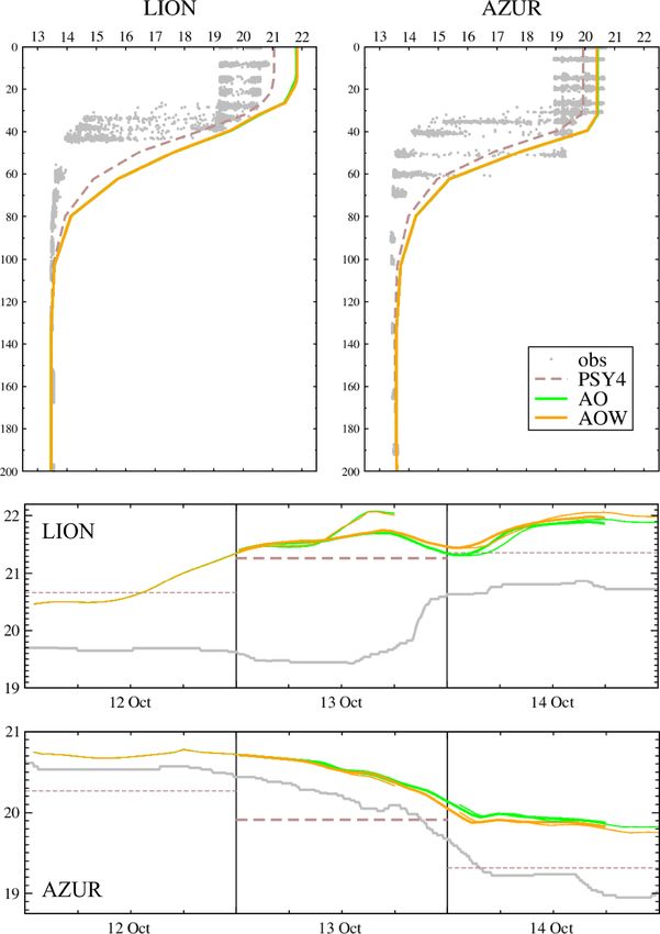
11864                                C. Sauvage et al.: Towards kilometer-scale ocean–atmosphere–wave coupled forecast

conditions come from the AROME-France analysis, and in            AYSSTatl simulations. The PSY4 SST from an ocean model
particular the SST field seen by AROME-France outside the         at 1/12◦ resolution enables us to represent finer structures in
northwestern Mediterranean area (NWM hereafter, Fig. 3a).         the Atlantic Ocean (Fig. 3) compared to the AROME anal-
The boundary conditions are provided by the hourly fore-          ysis, which only represents an average structure of the SST
cast from the Météo-France global model, ARPEGE (Action           field. Differences in the Atlantic Ocean can be as high as 2 ◦ C
de Recherche Petite Echelle Grande Echelle, Courtier et al.,      (3 ◦ C locally). This simulation is in fact an intermediate sim-
1991). For NEMO-NWMED72, the open boundary condi-                 ulation justified by the fact that the coupling with NEMO-
tions come from the global PSY4 daily analyses of Merca-          NWMED72 leads to changes in SST only in the Mediter-
tor Océan International at 1/12◦ resolution (Lellouche et al.,    ranean Sea. The comparison between AY and AYSSTatl thus
2018). The initial conditions come from a spin-up of NEMO-        allows for an assessment of the impact of the Atlantic Ocean
NWMED72 driven by AROME-France hourly flux forecasts              surface temperature on the HPE forecast.
(from 0 to +24 h each day starting on 5 October 2016) for the        A summary of the sea surface conditions for each experi-
forecast starting at 00:00 UTC on 12 October. For the sub-        ment is given in Table 2. The simulations AY and AW have
sequent forecasts, the ocean initial conditions at 00:00 UTC      already been used and validated in Sauvage et al. (2020) and
(day D) are provided by the AOW (ocean) forecast based            serve here as references to evaluate the coupling impact.
on the previous day (D − 1; range +24 h) through a restart.          Note that the insertion of ocean coupling here induces
The WW3-NWMED72 boundary conditions consist of eight              not only a prognostic evolution of the sea surface, but also
spectral points distributed along the domain and provided by      modifications of the initial SST conditions seen by AROME-
a WW3 global 1/2◦ resolution simulation (Rascle and Ard-          France over the NWM domain (Fig. 3c). These differences
huin, 2013) run at Ifremer. Wave initial conditions are restart   are induced by both the spin-up strategy and the restart mode
files, first from a former WW3 simulation for the forecast        of NEMO for each forecast run. Indeed, the spin-up (with-
starting at 00:00 UTC on 12 October and then from the pre-        out assimilation) makes NEMO-NWMED72 slowly diverg-
vious AOW forecast (D−1; range +24 h) for the following           ing from PSY4 but also allows it to produce its own fine-
days (see Sauvage et al., 2020, for a more detailed descrip-      scale structures permitted by its resolution (1/72◦ ) and in re-
tion of the wave initial and boundary conditions). Outside the    sponse to the AROME-France high-resolution atmospheric
NWM domain, the wave peak period field is estimated as a          forcing, whereas directly using the PSY4 3D fields would
function of the surface wind, and surface current is consid-      have let the ocean model adjustment affect the short-range
ered to be null.                                                  forecast. The choice to restart NEMO for coupled forecasts
   An atmosphere–wave coupled simulation (AW) was car-            from the spin-up first and then from a previous forecast was
ried out using AROME and WW3. The initial and boundary            also made to be close to the cycling done in an operational
conditions for waves and atmosphere are treated as in AOW.        context, i.e., using a previous forecast as initial conditions
The initial SST field comes from the PSY4 daily analysis of       for the surface scheme (and as a background for the AROME
the starting day of the forecast and is kept constant through-    3D-Var data assimilation scheme, not done here). This way,
out the 42 h of forecast. Surface currents are considered null.   the ocean model is initialized with adjusted, fine-scale, and
Coupling only takes place in the NWM domain. Elsewhere,           instantaneous fields, which are representative of ocean condi-
Tp is computed as a function of the surface wind.                 tions in the Mediterranean Sea before the event, while larger-
   The AO experiment is the coupled ocean–atmosphere sim-         scale daily-mean SST conditions are applied in fact in AY,
ulation between AROME and NEMO. The initial and bound-            AYSSTatl and AW with the PSY4 SST analyses.
ary conditions for ocean and atmosphere are treated as in            Thus, regarding the study of Sauvage et al. (2020), the
AOW. Outside the NWM domain, the SST is given by the              tri-coupling presented here adds new sea surface conditions,
AROME-France analyses, and the surface current is consid-         with the interactive evolution of the SST and of the currents
ered null. Everywhere, Tp is computed as a function of the        simulated by NEMO at a kilometric resolution taken into ac-
surface wind.                                                     count in the turbulent fluxes during the HPE forecast. This
   Two atmosphere-only experiments with AROME-France              permits us (1) to verify the robustness of the results obtained
are also examined using the same atmospheric boundary and         on wave coupling impact, when an interactive ocean is in-
initial conditions as AOW but different SSTs. In the AY           cluded, and (2) to investigate and compare the coupling con-
experiment, the SST initial field is taken from the PSY4          tributions to HPE forecast.
daily analyses for the whole marine domain of AROME-                 In order to quantify the impacts of coupling, a sensitivity
France, whereas in AYSSTatl, the SST forcing comes from           analysis is conducted by finely analyzing the differences ob-
the PSY4 analyses only on the NWM domain and from the             tained. In particular, the contribution of the tri-coupled sys-
AROME-France analyses elsewhere. Both AY and AYSSTalt             tem (ocean–atmosphere–wave) will be compared to the im-
use WASP as turbulent flux parameterization with the peak         pacts of the bi-coupled simulations (i.e., ocean–atmosphere
period estimated as a function of the surface wind, a con-        and wave–atmosphere). The method thus consists in compar-
stant SST field during the forecast and null current. Fig-        ing the simulations two by two by estimating the impacts of
ure 3b shows the differences in SST between the AY and            the coupling (interactive evolution and changes in the initial

Atmos. Chem. Phys., 21, 11857–11887, 2021                                         https://doi.org/10.5194/acp-21-11857-2021
C. Sauvage et al.: Towards kilometer-scale ocean–atmosphere–wave coupled forecast 11865
Table 2. Summary of the simulations. Outside the northwestern Mediterranean (NWM) area, surface current is always null and Tp is a
function of the wind (Ua ) only.
Models SST (outside NWM) SST (over NWM) Currents (over NWM) Tp (over NWM)
AY AROME PSY4 Null f (Ua )
AYSSTatl AROME AROME analysis PSY4 Null f (Ua )
AO AROME-NEMO AROME analysis Coupled f (Ua )
Initially NEMO spin-up for 12 October,
then AO D − 1 +24 h forecast
AW AROME-WW3 PSY4 Null Coupled
AOW AROME-NEMO-WW3 AROME analysis Coupled Coupled
Initially NEMO spin-up for 12 October,
then AOW D − 1 +24 h forecast
Table 3. Scores against observations from moored buoys and surface weather stations for the 10 m wind speed (WSP, m s−1 ), the 10 m wind
direction (WDIR, ◦ ), the air temperature at 2 m (T2M ◦ C) and the relative humidity at 2 m (RH2M, %).
WSP WDIR T2M RH2M
Bias RMSE Corr. Bias RMSE Corr. Bias RMSE Corr. Bias RMSE Corr.
AY 0.22 2.70 0.66 1.43 42.05 0.85 0.39 1.25 0.70 2.19 8.84 0.79
AYSSTatl 0.24 2.69 0.66 1.29 42.61 0.86 0.4 1.25 0.71 2.24 8.88 0.78
AO 0.28 2.74 0.65 2.65 42.14 0.85 0.53 1.34 0.71 1.97 9.03 0.77
AW 0.09 2.67 0.65 1.85 42.95 0.85 0.44 1.32 0.66 3.0 9.97 0.76
AOW 0.1 2.71 0.65 1.99 42.8 0.88 0.57 1.4 0.67 2.55 9.8 0.75
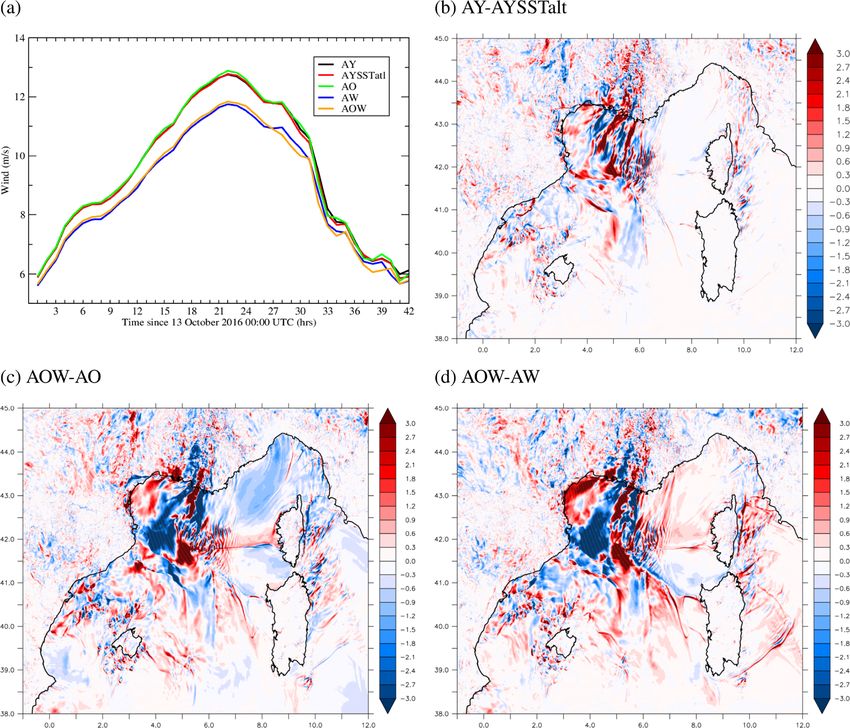
conditions brought by coupling) on the dynamics (wind) and cantly reducing the wind speed along the French Riviera, up
the low-level environment (temperature, humidity), the tur- to 3 m s−1 and by 7 % in average with notably a decrease in
bulent surface fluxes (momentum flux (or wind stress), sen- bias at the Azur buoy. This is reflected in the overall wind
sible heat flux H and latent heat flux LE), evaporation and speed bias in Table 3 presenting the bias, RMSE (root mean
precipitation. When available, observations of the air–sea in- square error) and correlation coefficient calculated for each
terface are also used to qualify the different simulations. The experiment with respect to weather surface stations. A spatial
impacts of tri-coupling on the representation of the surface shift of about 15 km eastward of the convergence line and of
ocean layer and the sea state (Hs and Tp ) are also examined. heavy precipitation at sea is found, linked to the slowdown
of the easterly wind upstream (along the French Riviera). In
AW, a decrease in latent and sensible heat fluxes was noticed
4 Coupling impact on forecast compared to AY. However, this decrease was only ∼ 2 % on
the total turbulent heat flux, despite a priori favorable condi-
4.1 Atmosphere–wave coupling tions for a larger response (i.e., strong winds, a large air–sea
thermal gradient, and a young sea). Wave coupling also leads
The analysis of the atmosphere–wave coupling is described
to significant differences in the Gulf of Lion, downstream of
in detail in Sauvage et al. (2020) with comparison of AW
the convective system over the sea, related to internal mod-
(AWC in Sauvage et al., 2020) to AY. Here are some high-
ifications of the convective system. Finally, the convective
lights of the main conclusions.
system over the Hérault area appears not sensitive to wave
The main result is a significant increase in the wind stress
coupling (or forcing). This can be explained by the fact that
found along the French Riviera where the low-level wind
orographic uplift is the triggering factor of this system.
is the strongest, as taking into account the sea state with
Adding the coupling with waves to an atmosphere–ocean
the generation of a wind sea leads to an increase in sur-
coupled configuration can impact the heat extraction from
face roughness. The increase in stress in this region repre-
the ocean in several manners (e.g., Renault et al., 2012; Var-
sents +10 % during Phase I (between 13 October 03:00 and
las et al., 2020). First, taking into account waves can in-
18:00 UTC) and +8.6 % during Phase II (between 13 Oc-
crease the surface roughness, leading to larger wind stress
tober 19:00 UTC and 14 October 03:00 UTC) when com-
and weaker surface wind. This decrease in the wind can di-
pared to AY. The wave coupling has the effect of signifi-
https://doi.org/10.5194/acp-21-11857-2021 Atmos. Chem. Phys., 21, 11857–11887, 2021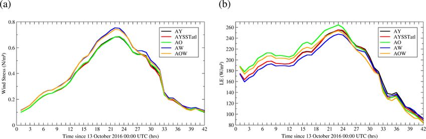
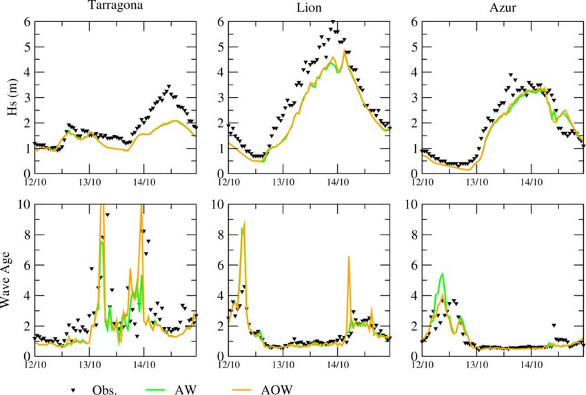
11866                                C. Sauvage et al.: Towards kilometer-scale ocean–atmosphere–wave coupled forecast

rectly decrease the heat fluxes (see Eq. 5). Then, the increase    Table 4. Simulated maximum and mean values of rainfall amounts
in the surface roughness can result in larger transfer coeffi-     (mm) in 24 h at 00:00 UTC on 14 October over the Hérault zone
cients for heat (Eq. 8) that can lead to slightly larger heat      and the offshore zone around MCSs for the different experiments
fluxes. Finally, even though the ocean and wave models are         (forecast starting at 00:00 UTC on 13 October).
not directly coupled in the present study, stronger wind stress
can result in more mixing and cooling in the oceanic surface                           Zone 1 (Hérault)      Zone 2 (sea)
layer and thus colder SSTs. These colder SSTs can dampen                              Maximum Mean         Maximum Mean
the turbulent heat fluxes directly and also increase the atmo-           AY             273.4      58.8      214.1      42.2
spheric stability at a low level, further decreasing the surface         AYSSTatl       269.7      57.2      176.5      42.4
wind and eventually the turbulent heat fluxes. In the present            AO             306.2      60.9      196.5      43.5
case, coupling with waves has almost no impact on SST (dif-              AW             271.9      56.8      188.1      43.5
ferences of less than 0.2 ◦ C, not shown). The impact of the             AOW            264.6      58.4      228.8      45.1
z0 increase on the heat transfer coefficients is also negligi-           ANTILOPE       287.9      73.2      348.2      51.6
ble (not shown). Conversely, the decrease in the simulated
wind between AO and AOW is comparable to what was ob-
tained between AY and AW and significant during Phases I           tation is seen. Since the near-surface wind in AOW decreases
and II, with differences of more than 1 m s−1 over a large         (compared to AO) in the same way as in AW (compared to
area along the French Riviera (Figs. 4c and 2a for the loca-       AY), this shift in the location of the convergence and heavy
tion). As a result, latent and sensible heat fluxes are reduced    precipitation at sea is likely due to the same process, i.e., a
in AOW by 3 % over Phases I and II (Figs. 5b and 6c, d),           higher roughness in the Ligurian Sea and a slowdown of the
i.e., a slightly larger decrease than in AW/AY because of the      easterly low-level atmospheric flow.
nonlinear response of the heat fluxes to more unstable con-           Comparisons with sea state recorded by moored buoys are
ditions in AOW/AO, and are mainly due to the slowdown of           additionally used to assess the quality of the wave forecast in
the wind. This result is in contrast with what was obtained in     AOW and AW simulations. The scores calculated for the sea
other case studies (e.g., Varlas et al., 2020), probably because   state parameters are summarized in Table 5. Few differences
the surface wind and the mixing in the oceanic mixed layer         in Hs and Tp scores are obtained when comparing AOW to
were much stronger than here.                                      AW, with a reduction in bias for moored buoys, a reduction in
   Figure 7a presents different probability scores accord-         RMSE for Tp , and a slight decrease in correlation in AOW.
ing to 24 h precipitation accumulation (between 13 October         The evolution of the sea state during the event is described
00:00 UTC and 14 October 00:00 UTC) thresholds (Ducrocq            for three moored buoys – Tarragona, Lion and Azur – in
et al., 2002): ACC (accuracy), POD (probability of detec-          Fig. 9. The Hs time series simulated by AOW and AW are
tion), FAR (probability of false alarm), FBIAS (frequency          very close. Nevertheless, we observe a trend of increasing
bias), ETS (equitable threat score) and HSS (Heidke skill          values of Hs and Tp in AOW, with for example for Hs + 20–
score) are calculated by comparison to rain-gauge observa-         40 cm locally in the Gulf of Lion and along the French Riv-
tions shown in Fig. 7b. The FAR score is better when it is         iera that represents an increase on the order of 1 %–2 % on
close to 0; for the others, a score of 1 is relative to a per-     average in these areas.
fect prediction. Precipitation scores between AOW and AO              The differences in Hs are larger around 00:00 UTC on
are close for cumulative thresholds between 0 and 50 mm.           14 October, particularly under the convective system. A dif-
More variability appears for higher thresholds, but overall        ference dipole of ±1 m corresponds in fact to a shift of the
AO performs better than AOW. The addition of wave cou-             maximum Hs values due to the different positioning of the
pling slightly reduces the intensity of precipitation over the     MCS at sea at that time between AOW and AW. The time
Hérault area on average and with a maximum 24 h amount             series of the wave age during this period show small changes
in AOW of 264 mm compared to AO with 306 mm (Table 4).             between the simulations (Fig. 9), and we conclude that the
Except for this punctual decrease in the maximum, the heavy        characteristics of the sea state forecast remain the same in
rainfall event over Hérault in AOW is very similar to the          AW and AOW, with a wind sea (corresponding to wave
one in AO (chronology, area and mean amount, Fig. 8c; see          age < 1) well represented at Lion and Azur.
Fig. 2c for the location), and so there is no degradation due to
the inclusion of the wave coupling from a NWP and/or early         4.2    Atmosphere–ocean coupling
warning perspective.
   For precipitation related to the MCS over the sea, the wave     As stated in Sect. 3.2, introducing the ocean coupling con-
coupling induces larger mean values when comparing AOW             sists of an interactive ocean model and a change in the ini-
with AO (Table 4). Figure 8c shows the differences in the 6 h      tial SST condition. Figure 3c represents the difference in ini-
accumulation of precipitation at 00:00 UTC on 14 October           tial SST in the Mediterranean at 00:00 UTC on 13 October
between AOW and AO, i.e., during Phase II. A slight east-          between AOW and AW (i.e., the PSY4 analysis). The ini-
ward shift of a few kilometers in the location of the precipi-     tial SST is warmer in AOW, especially in the Gulf of Lion,

Atmos. Chem. Phys., 21, 11857–11887, 2021                                           https://doi.org/10.5194/acp-21-11857-2021
C. Sauvage et al.: Towards kilometer-scale ocean–atmosphere–wave coupled forecast                                                   11867

Figure 4. (a) Time series of the surface wind (m s−1 ) forecasts on average over the Azur area and differences in surface wind at 00:00 UTC
on 14 October between (b) AY and AYSSTatl, (c) AOW and AO and (d) AOW and AW (forecast basis: 13 October 00:00 UTC).

Table 5. Scores against wave observations from moored buoys and satellites for Hs (m) and Tp (s).

                                                    Moored buoys                                Satellites
                                            Hs                          Tp                         Hs
                                  Bias     RMSE      Corr.    Bias     RMSE      Corr.     Bias  RMSE        Corr.
                        AW       −0.28      0.58     0.90    −1.27      1.64     0.88     −0.28      0.5     0.71
                        AOW      −0.22      0.61     0.89    −0.87      1.34     0.85     −0.28      0.5     0.72

along the French Riviera and in the Tyrrhenian Sea (up to               evaporation and latent heat flux are found in AOW compared
1.5 ◦ C). At 00:00 UTC on 14 October, after 24 h of forecast,           to AW (+7 % in the Azur zone during Phase I, Figs. 5b and
the SST in AOW cooled down (Fig. 3d), especially in the                 6a, b) due to a warmer SST at the beginning of the event. The
Gulf of Lion and along the French Riviera where winds and               sensible heat flux in AOW is also increased by 11 % during
heat fluxes are strongest (Fig. 2a, b). In these areas, larger          Phases I and II compared to AW (not shown). This allows

https://doi.org/10.5194/acp-21-11857-2021                                                Atmos. Chem. Phys., 21, 11857–11887, 2021
11868 C. Sauvage et al.: Towards kilometer-scale ocean–atmosphere–wave coupled forecast
Figure 5. Time series of (a) wind stress (N m−2 ) and (b) latent heat flux (LE, W m−2 ) on average over the Azur area for forecasts starting at
00:00 UTC on 13 October.
more heat and moisture extraction from the ocean mixed Coupling with the ocean results in more intense precipita-
layer to the atmospheric low levels and therefore more favor- tion for the system on the Hérault with a larger mean rainfall
able low-level conditions for convective systems. In the last amount (Table 4 and Fig. 8b) and a maximum 24 h rainfall
part of the event, coupling with the ocean results in slightly amount at 00:00 UTC on 14 October of 306 mm in AO ver-
colder SSTs in AOW than in AW and slightly lower enthalpy sus 269 mm in AYSSTatl. This is due to a slightly moister and
fluxes. Ocean coupling appears to have a small impact on warmer air mass at low levels over the Gulf of Lion leading
wind stress and surface wind speed: both simulated parame- to a more intense convection. At sea, an increase in the max-
ters in AOW are on average identical to those of AW along imum 24 h rainfall amount is obtained in AOW (228 mm)
the French Riviera and in the Gulf of Lion, with differences compared to AW (188 mm) (and in AO (196 mm) compared
of less than 0.3 m s−1 (Figs. 5a and 4a, d). The largest differ- to AYSSTatl – 176 mm), but the mean value remains close.
ences are found in the Gulf of Lion in the form of dipoles that Overall, rainfall scores are better in AO (and AOW) com-
are not homogeneous in time. These patches of differences pared to AYSSTatl (and AW) (Fig. 7b). The differences in
are mainly due to modifications in the evolution of convec- the 6 h accumulation of precipitation at 00:00 UTC on 14 Oc-
tive cells and small displacements of the MCS over the sea tober between AOW and AW appear quite similar to those
in the different simulations, with consequences for the low- between AOW and AO, especially for the offshore system
level flow downstream. The same results are observed when (Fig. 8c, d), because of a slight eastward shift of a few
comparing heat fluxes and surface dynamics between AO and kilometers in the location of the precipitation. The effect of
AYSSTatl. In view of these results, it confirms that ocean ocean coupling on precipitation, however, involves a differ-
coupling including change in the initial SST and taking into ent mechanism than wave coupling. Indeed, the addition of
account the interactive SST and surface currents in the wind the ocean coupling with a warmer initial SST allows for a
stress computation has a very low impact on the near-surface larger input of heat and moisture due to higher evaporation
wind for such a strong wind regime largely controlled by the and heat fluxes during the initiation phase. This leads to an
synoptic circulation. intensification of the system at sea with formation of a cold
For temperature (T2M) and relative humidity (RH2M) at pool, which reinforces and tends to push eastwards the con-
2 m, small differences are obtained on average between the vergence during the mature phase (Fig. 10).
simulations. T2M varies from 1 % to 3 % on average with a The strong sensitivity of the convergence at sea to changes
tendency to increase for T2M when the atmosphere is cou- in initial SST and to the oceanic feedback was already high-
pled with the ocean (and/or waves). For RH2M, coupling lighted by Rainaud et al. (2017) with the AROME-NEMO
with the ocean has a small impact (< 1 %) that in fact cor- coupling for another Mediterranean HPE. The present study
responds to an increase in the specific humidity at 2 m (not permits us to identify more clearly the large impact of ocean
shown) associated with the low-level warming. Although initialization and coupling on heat and water supply, which
these differences are, on average, not significant, larger dif- controls the intensity of convection which itself modifies the
ferences can be observed at any given time along the French MCS motion and location through internal mechanisms act-
Riviera and under the convective system in the Gulf of Lion ing for this case to a convergence reinforcement.
(not shown). Concerning ocean forecasts, AOW and AO simulations
show very similar results, with a positive bias in tempera-
Atmos. Chem. Phys., 21, 11857–11887, 2021 https://doi.org/10.5194/acp-21-11857-2021C. Sauvage et al.: Towards kilometer-scale ocean–atmosphere–wave coupled forecast 11869 Figure 6. LE differences (W m−2 ) (a, c) at 14:00 UTC on 13 October and (b, d) at 00:00 UTC on 14 October between AOW and AW experiments (a, b) and between AOW and AO experiments (c, d). ture (0.57 ◦ C) and almost null in salinity (−0.02 psu) when and especially that the thermocline is less marked than ob- compared to moored and drifting buoy observations between served. The same defect of a less marked thermocline (halo- 12 October 00:00 UTC and 15 October 00:00 UTC (using cline) is found in the analyses of the ocean operational sys- the +1 to +24 h forecast ranges for each day). The ther- tem PSY4 when compared to the same observations, which mohaline characteristics of intermediate and deep waters shows that the biases of AOW and AO are in fact largely are very well represented. If we consider only the upper- inherited from the ocean initial state used. Also, Fig. 11 ocean layer (0–100 m), the biases are larger (about −1 ◦ C shows the cooling at the Azur buoy under the strong east- and −0.05 psu, respectively). The most important errors are erly wind observed all along the event (−0.75 ◦ C in 24 h and located between about 15 and 60 m, with biases up to 6 ◦ C −1.4 ◦ C in 42 h observed since 00:00 UTC on 13 October). and −0.9 psu. These large differences actually reflect an is- This ocean response appears quite large considering other sue in the representation of the thermocline and halocline, HPE studies (e.g., Lebeaupin Brossier et al., 2009, 2014; which are deeper but also smoother in the model. Figure 11, Rainaud et al., 2017) and is comparable to other high-wind comparing the simulated temperature profiles at the Lion and or medicane events (e.g., Renault et al., 2012; Bouin and Azur buoys, shows indeed that the mixed layer is thicker Lebeaupin Brossier, 2020a). Even though it is significant, it https://doi.org/10.5194/acp-21-11857-2021 Atmos. Chem. Phys., 21, 11857–11887, 2021
11870                                   C. Sauvage et al.: Towards kilometer-scale ocean–atmosphere–wave coupled forecast

Figure 7. (a) Locations and measurements of 24 h cumulative precipitation (mm) at 00:00 UTC on 14 October of the Météo-France rain
gauges over the southeastern quarter of France. (b) Forecast skill scores against rain-gauge observations calculated for cumulative rainfall in
24 h at 00:00 UTC on 14 October. The x axis indicates the rainfall threshold considered, in millimeters.

Atmos. Chem. Phys., 21, 11857–11887, 2021                                                   https://doi.org/10.5194/acp-21-11857-2021
C. Sauvage et al.: Towards kilometer-scale ocean–atmosphere–wave coupled forecast                                         11871

Figure 8. Differences in 6 h cumulative precipitation (mm) at 00:00 UTC on 14 October (a) between AOW and AO and (b) between AOW
and AW.

appears to be underestimated by the model (−0.6 ◦ C in 24 h       Azur area (Figs. 5 and 6). Here and all along the two phases,
and −0.85 ◦ C in 42 h simulated by AOW). Overall, this de-        the low-level wind is reduced upstream of the offshore MCS
fault in representing the cooling can be explained by the ini-    (Fig. 4). As a consequence of larger heat and moisture sup-
tial ocean state with a too smooth thermocline that limits the    plies, both convective systems over Hérault and over the sea
mixed-layer cooling by entrainment, by physical parameters        are more intense and lead to larger precipitation amount fore-
and/or schemes in NEMO and by the absence of ocean–wave           cast (Fig. 8 and Table 4). In AOW, the more intense MCS
coupling.                                                         over the sea tends to reinforce the convergence (Fig. 10),
                                                                  which is displaced by nearly 100 km eastwards compared to
                                                                  AY.
5   Discussion                                                       In fact, the analysis of the coupled simulations AW, AOW,
                                                                  and AO shows the high sensitivity of the location of the heavy
The comparison of the AOW tri-coupled experiment with             precipitating MCS at sea, as an eastward shift of several kilo-
the AY atmosphere-only experiment highlights that the com-        meters of the system is seen with any coupling (Fig. 8). How-
bined effect of couplings is an increase in wind stress and       ever, the mechanisms identified for this response appear dif-
enthalpy flux during the initiation and mature phases in the

https://doi.org/10.5194/acp-21-11857-2021                                       Atmos. Chem. Phys., 21, 11857–11887, 2021
11872 C. Sauvage et al.: Towards kilometer-scale ocean–atmosphere–wave coupled forecast Figure 9. Time series of simulated significant wave height Hs and wave age at the three moored buoys Tarragona, Lion and Azur at 00:00 UTC on 12 October to 00:00 UTC on 15 October, using successive forecasts of each experiment including WW3 (+1–+24 h forecast ranges each day). ferent between wave coupling and ocean coupling. On the Baltic Sea that taking into account the effect of waves on one hand, the dominant process with wave coupling is the the ocean improved surface temperature, ocean surface cir- slowing down of the easterly flow due to more roughness culation and sea level height. So, it would be interesting to that shifts the location of the convergence line, whatever the conduct other experiments by adding the interactive cou- surface heat flux values are (related to SST or low-level wind pling between ocean and waves, as it would likely modify variations). On the other hand, ocean coupling and its ini- the turbulence and the exchanges at the air–sea interface. The tialization strongly control the heat and moisture supply that use of the SURFEX-OASIS coupling interface enables us to indirectly impacts the convergence through internal modifi- quickly consider the insertion of the full coupling between cations of the convective system (more intense if a higher NEMO and WW3, as recently developed by Couvelard et al. SST is used during the initiation and mature stages). Thus, (2020) with updates in the physics of NEMO (v3.6) and val- these results prove the importance and complementarity of idated through a global coupled modeling study. As men- both couplings to well represent the complex interactions of tioned in Sect. 4.2, the SST initial field is of great importance the ocean upper and surface layers with the marine atmo- for short-term forecast of extreme events involving large air– spheric boundary layer, in particular for such severe weather sea fluxes (e.g., Lebeaupin Brossier et al., 2009; Rainaud conditions with large exchanges. et al., 2017). The spin-up strategy used to start NEMO in the The clear splitting between the two coupling impacts on AO- and AOW-coupled simulations induced large discrep- the atmospheric event here has been done thanks to bi- ancies when compared to the PSY4 daily analysis (Fig. 3) coupled experiments and confirmed in AOW, where there is as in AROME-only simulations (AY or AYSSTatl). On the no direct interaction between ocean and waves. However, it other hand, the use of the PSY4 SST daily analysis to start has been shown that surface waves enhanced vertical mix- the forecast means that initial conditions (i.e., at 00:00 UTC) ing in the ocean surface layer. In the case of tropical cy- are actually a 24 h average of the SST, including changes in clones, Aijaz et al. (2017) for example showed that wave- SST due to the studied event. To better illustrate this initial- induced mixing caused significant cooling and a deepening ization issue, the comparison of the 6 m-depth temperature at of the mixing layer, which can then impact the intensity Azur in Fig. 11 shows that starting with the PSY4 analysis on of the cyclone. Staneva et al. (2016) and Wu et al. (2019) 13 October leads to a significant initial cold bias compared to also showed with sensitivity studies in the North Sea and observations (−0.5 ◦ C, similarly for SST) as PSY4 already Atmos. Chem. Phys., 21, 11857–11887, 2021 https://doi.org/10.5194/acp-21-11857-2021
You can also read