Global-scale distribution of ozone in the remote troposphere from the ATom and HIPPO airborne field missions
←
→
Page content transcription
If your browser does not render page correctly, please read the page content below
Atmos. Chem. Phys., 20, 10611–10635, 2020
https://doi.org/10.5194/acp-20-10611-2020
© Author(s) 2020. This work is distributed under
the Creative Commons Attribution 4.0 License.

Global-scale distribution of ozone in the remote troposphere from
the ATom and HIPPO airborne field missions
Ilann Bourgeois1,2 , Jeff Peischl1,2 , Chelsea R. Thompson1,2 , Kenneth C. Aikin1,2 , Teresa Campos3 , Hannah Clark4 ,
Róisín Commane5 , Bruce Daube6 , Glenn W. Diskin7 , James W. Elkins8 , Ru-Shan Gao2 , Audrey Gaudel1,2 ,
Eric J. Hintsa1,8 , Bryan J. Johnson8 , Rigel Kivi9 , Kathryn McKain1,8 , Fred L. Moore1,8 , David D. Parrish1,2 ,
Richard Querel10 , Eric Ray1,2 , Ricardo Sánchez11 , Colm Sweeney8 , David W. Tarasick12 , Anne M. Thompson13 ,
Valérie Thouret14 , Jacquelyn C. Witte3 , Steve C. Wofsy6 , and Thomas B. Ryerson2
1 Cooperative Institute for Research in Environmental Sciences, University of Colorado Boulder,
Boulder, CO, USA
2 NOAA Chemical Science Laboratory, Boulder, CO, USA
3 National Center for Atmospheric Research, Boulder, CO, USA
4 IAGOS-AISBL, Brussels, Belgium
5 Department of Earth and Environmental Sciences, Lamont-Doherty Earth Observatory of Columbia University,

New York, NY, USA
6 School of Engineering and Applied Sciences, Harvard University, Cambridge, MA, USA
7 NASA Langley Research Center, Hampton, VA, USA
8 NOAA Global Monitoring Laboratory, Boulder, CO, USA
9 Finnish Meteorological Institute, Space and Earth Observation Centre, Sodankylä, Finland
10 National Institute of Water & Atmospheric Research (NIWA), Lauder, New Zealand
11 Servicio Meteorológico Nacional, Buenos Aires, Argentina
12 Experimental Studies Research Division, MSC/Environment and Climate Change Canada,

Downsview, Ontario, Canada
13 Earth Sciences Division, NASA Goddard Space Flight Center, Greenbelt, MD, USA
14 Laboratoire d’Aérologie, CNRS and Université Paul Sabatier, Université de Toulouse, Toulouse, France

Correspondence: Ilann Bourgeois (ilann.bourgeois@noaa.gov) and Jeff Peischl (jeff.peischl@noaa.gov)

Received: 1 April 2020 – Discussion started: 14 April 2020
Revised: 17 July 2020 – Accepted: 25 July 2020 – Published: 11 September 2020

Abstract. Ozone is a key constituent of the troposphere,         the troposphere, with HIPPO sampling the atmosphere over
where it drives photochemical processes, impacts air quality,    the Pacific and ATom sampling both the Pacific and Atlantic.
and acts as a climate forcer. Large-scale in situ observations   Given the relatively limited temporal resolution of these two
of ozone commensurate with the grid resolution of current        campaigns, we first compare ATom and HIPPO ozone data
Earth system models are necessary to validate model outputs      to longer-term observational records to establish the repre-
and satellite retrievals. In this paper, we examine measure-     sentativeness of our dataset. We show that these two airborne
ments from the Atmospheric Tomography (ATom; four de-            campaigns captured on average 53 %, 54 %, and 38 % of the
ployments in 2016–2018) and the HIAPER Pole-to-Pole Ob-          ozone variability in the marine boundary layer, free tropo-
servations (HIPPO; five deployments in 2009–2011) experi-        sphere, and upper troposphere–lower stratosphere (UTLS),
ments, two global-scale airborne campaigns covering the Pa-      respectively, at nine well-established ozonesonde sites. Ad-
cific and Atlantic basins.                                       ditionally, ATom captured the most frequent ozone concen-
   ATom and HIPPO represent the first global-scale, verti-       trations measured by regular commercial aircraft flights in
cally resolved measurements of O3 distributions throughout       the northern Atlantic UTLS. We then use the repeated verti-

Published by Copernicus Publications on behalf of the European Geosciences Union.
10612                                       I. Bourgeois et al.: Global-scale distribution of ozone in the remote troposphere

cal profiles from these two campaigns to confirm and extend        iment (GTE), a major component of the National Aeronau-
the existing knowledge of tropospheric ozone spatial and           tics and Space Administration (NASA) Tropospheric Chem-
vertical distributions throughout the remote troposphere. We       istry Program (https://www-gte.larc.nasa.gov, last access:
highlight a clear hemispheric gradient, with greater ozone in      9 April 2020). Airborne campaigns have targeted both the
the Northern Hemisphere, consistent with greater precursor         Pacific and Atlantic oceans, providing novel characterization
emissions and consistent with previous modeling and satel-         of O3 sources, distribution, and photochemistry in the marine
lite studies. We also show that the ozone distribution below       troposphere (Browell et al., 1996a; Davis et al., 1996; Jacob
8 km was similar in the extra-tropics of the Atlantic and Pa-      et al., 1996; Pan et al., 2015; Schultz et al., 1999; Singh et
cific basins, likely due to zonal circulation patterns. However,   al., 1996c) and the low-O3 tropical Pacific pool (Singh et al.,
twice as much ozone was found in the tropical Atlantic as in       1996b); the pervasive role of continental outflow on O3 pro-
the tropical Pacific, due to well-documented dynamical pat-        duction (Bey et al., 2001; Crawford et al., 1997; Heald et
terns transporting continental air masses over the Atlantic.       al., 2003; Kondo et al., 2004; Martin et al., 2002; Zhang et
Finally, we show that the seasonal variability of tropospheric     al., 2008); and the marked influence of African and South
ozone over the Pacific and the Atlantic basins is driven year-     American biomass burning on O3 production in the South-
round by transported continental plumes and photochemistry,        ern Hemisphere (Browell et al., 1996b; Fenn et al., 1999;
and the vertical distribution is driven by photochemistry and      Mauzerall et al., 1998; Singh et al., 1996a; Thompson et al.,
mixing with stratospheric air. This new dataset provides ad-       1996). Ozonesondes have been launched from remote sites
ditional constraints for global climate and chemistry models       for more than 3 decades in some places and have provided
to improve our understanding of both ozone production and          additional constraints on the sources and photochemical bal-
loss processes in remote regions, as well as the influence of      ance of tropospheric O3 , including a deep understanding of
anthropogenic emissions on baseline ozone.                         the vertically resolved tropospheric O3 climatology in select
                                                                   locations (Derwent et al., 2016; Diab et al., 2004; Jensen et
                                                                   al., 2012; Kley et al., 1996; Liu et al., 2013; Logan, 1985; Lo-
                                                                   gan and Kirchhoff, 1986; Newton et al., 2018; Oltmans et al.,
1   Introduction                                                   2001; Parrish et al., 2016; Sauvage et al., 2006; Thompson et
                                                                   al., 2012). Spatially resolved O3 climatology has been pro-
Tropospheric ozone (O3 ) plays a major role in local, regional,    vided from routine sampling by commercial aircraft, which
and global air quality and significantly influences Earth’s ra-    has mostly been limited to the upper troposphere or over con-
diative budget (IPCC, 2013; Shindell et al., 2012). In ad-         tinental regions (Clark et al., 2015; Cohen et al., 2018; Logan
dition, O3 drives tropospheric photochemical processes by          et al., 2012; Petetin et al., 2016; Sauvage et al., 2006; Thouret
controlling hydroxyl radical (OH) abundance, which sub-            et al., 1998; Zbinden et al., 2013), and by satellite obser-
sequently controls the lifetime of other pollutants includ-        vations (Edwards et al., 2003; Fishman et al., 1990, 1991;
ing volatile organic compounds (VOCs), methane, and some           Hu et al., 2017; Thompson et al., 2017; Wespes et al., 2017;
stratospheric ozone-depleting substances (Crutzen, 1974;           Ziemke et al., 2005, 2006, 2017), which have been somewhat
Levy, 1971). Sources of O3 to the troposphere include down-        tempered by large uncertainties (Tarasick et al., 2019b). Re-
ward transport from the stratosphere (Junge, 1962) and             cent overview analyses depict the current understanding of
photochemical production from precursors such as carbon            global tropospheric O3 sources, distribution, and photochem-
monoxide (CO), methane (CH4 ), and VOCs in the pres-               ical balance and underscore the insufficiency of observations
ence of nitrogen oxides (NOx ) from natural or anthropogenic       in the remote free troposphere (Cooper et al., 2014; Gaudel
sources (Monks et al., 2009). Tropospheric O3 sinks include        et al., 2018; Tarasick et al., 2019b) necessary to improve the
photodissociation, chemical reactions, and dry deposition.         current representation of tropospheric O3 in global chemical
Owing to its relatively long lifetime (∼ 23 d in the tropo-        models (Young et al., 2018). The spatial and temporal rep-
sphere; Young et al., 2013), O3 can be transported across          resentativeness of O3 observations is currently the biggest
hemispheric scales. Thus, O3 mixing ratios over a region de-       source of uncertainty when inferring O3 climatology in the
pend not only on local and regional sources and sinks but          free troposphere, even in regions where observation are abun-
also on long-range transport. Further, the uneven density of       dant but not ideally distributed (Lin et al., 2015b; Tarasick et
O3 monitoring locations around the globe leads to signifi-         al., 2019b). Most studies reporting the global O3 distribu-
cant sampling gaps, especially near developing nations and         tion use satellite observations (Edwards et al., 2003; Fish-
away from land (Gaudel et al., 2018). The troposphere over         man et al., 1990, 1991; Thompson et al., 2017; Wespes et al.,
the remote oceans is among the least-sampled regions, de-          2017; Ziemke et al., 2005, 2006, 2017), modeling analyses
spite hosting 60 %–70 % of the global tropospheric O3 bur-         (Hu et al., 2017), or observations spatially expanded using
den (Holmes et al., 2013).                                         back trajectory calculations (e.g., Liu et al., 2013; Tarasick
   Since the early 1980s, several aircraft campaigns have          et al., 2010). While useful, these studies come with some-
addressed this paucity of remote observations, most no-            what large uncertainties, as recently noted by reports from
tably under the umbrella of the Global Tropospheric Exper-         the Tropospheric Ozone Assessment Report (TOAR), and

Atmos. Chem. Phys., 20, 10611–10635, 2020                                          https://doi.org/10.5194/acp-20-10611-2020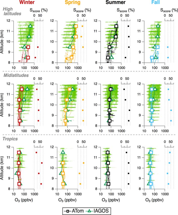
I. Bourgeois et al.: Global-scale distribution of ozone in the remote troposphere                                              10613

                                                                         Here we use existing ozonesonde and commercial aircraft
                                                                      observations of O3 at selected locations along the ATom and
                                                                      HIPPO circuits to provide a climatological context for the al-
                                                                      titudinal, latitudinal, and seasonal distributions of O3 derived
                                                                      from the systematic airborne in situ “snapshots”. Long-term
                                                                      O3 observations are obtained from decades of ozonesonde
                                                                      vertical profiles (e.g., Oltmans et al., 2013; Thompson et al.,
                                                                      2017) and from ∼ 60 000 flights using the In-service Air-
                                                                      craft for a Global Observing System (IAGOS) infrastruc-
                                                                      ture (Petzold et al., 2015; http://www.iagos.org, last access:
                                                                      9 April 2020). Ozonesondes have typically been launched
                                                                      weekly for 2 decades or more, depending on the site, and
                                                                      have sampled a wide range of air masses across the globe,
Figure 1. The location and flight tracks of all O3 monitoring plat-   from O3 -poor remote surface locations to the O3 -rich strato-
forms used in this work are illustrated using different markers and   sphere. IAGOS commercial aircraft have provided daily
colors. The ATom flight track is in black, the HIPPO flight track     measurements in the upper troposphere and lower strato-
is in blue, IAGOS flight paths are in green, and the ozonesonde       sphere (UTLS) for the past 25 years, especially over the
launching sites are indicated by the red markers. The dotted gray     northern midlatitudes between America and Europe. Com-
lines define the latitudinal bands over which individual ATom and     bined, the ozonesonde and IAGOS datasets offer robust
HIPPO profiles were averaged to derive a regional O3 distribution:    measurement-based climatologies that quantify the full ex-
the tropics (20◦ S–20◦ N), the midlatitudes (55–20◦ S, 20–60◦ N),     pected range of atmospheric O3 variability with altitude and
and the high latitudes (90–55◦ S, 60–90◦ N). Only data from remote    season.
oceanic flight segments of ATom and HIPPO missions were used in
                                                                         The in situ data from temporally limited intensive field
this work.
                                                                      studies can be placed in context by comparing them with
                                                                      long-term ozonesonde and commercial aircraft monitoring
                                                                      data. Evaluating the representativeness of in situ observations
thus require additional in situ observations to be used as a          from airborne campaigns by comparing them to longer-term
validation benchmark (Tarasick et al., 2019b; Young et al.,           observational records is a critical exercise never before done
2018).                                                                at such a global scale. We show that ATom and HIPPO mea-
   The Atmospheric Tomography (ATom, https://espo.nasa.               surements capture the spatial and, in some cases, temporal
gov/atom, last access: 9 April 2020) mission was a NASA               dependence of O3 in the remote atmosphere, thereby high-
Earth Venture airborne field project to address the sparse-           lighting the usefulness of airborne observations to fill in the
ness of atmospheric observations over remote ocean regions            gaps of established but limited O3 climatologies and other
by systematically sampling the troposphere over the Pacific           similarly long-lived species. Then, we use the geographically
and Atlantic basins along a global-scale circuit (Fig. 1).            extensive ATom and HIPPO vertical profile data to establish a
ATom deployed an extensive payload on the NASA DC-8                   more complete measurement-based benchmark for O3 abun-
aircraft, measuring a wide range of chemical, microphysi-             dance and distribution in the remote marine atmosphere.
cal, and meteorological parameters in repeated vertical pro-
files from 0.2 km to over 13 km in altitude, from the Arc-
tic to the Antarctic over the Pacific and Atlantic oceans, in         2     Measurements
four separate seasons from 2016 to 2018. ATom built on
                                                                      2.1    ATom
a previous study, the HIAPER Pole-to-Pole Observations
(HIPPO, https://www.eol.ucar.edu/field_projects/hippo, last           The four ATom circuits occurred in July–August 2016
access: 9 April 2020) mission. The goal of HIPPO was to               (ATom-1), January–February 2017 (ATom-2), September–
measure atmospheric distributions of important greenhouse             October 2017 (ATom-3), and April–May 2018 (ATom-4);
gases and reactive species over the Pacific Ocean, from the           thus, they spanned all four seasons in both hemispheres over
surface to the tropopause, five times during different sea-           a 2-year timeframe (Table S1 in the Supplement). In total,
sons from 2009 to 2011. Together, ATom and HIPPO pro-                 the mission consisted of 48 science flights and 548 verti-
vide recent and comprehensive information about the alti-             cal profiles distributed nearly equally along the global cir-
tudinal, latitudinal, and seasonal composition of the remote          cuit. All four deployments completed roughly the same loop,
troposphere over the Pacific, and ATom also provides this in-         starting and ending in Palmdale, California, USA (Fig. 1). A
formation over the Atlantic. In addition, ATom and HIPPO              notable addition during ATom-3 and ATom-4 were out-and-
sampling strategies were designed to deliver an objective cli-        back flights from Punta Arenas, Chile, to sample the Antarc-
matology of key species to enable the modeling of the air par-        tic troposphere and UTLS.
cel reactivity of the remote troposphere (Prather et al., 2017).

https://doi.org/10.5194/acp-20-10611-2020                                           Atmos. Chem. Phys., 20, 10611–10635, 2020
10614                                       I. Bourgeois et al.: Global-scale distribution of ozone in the remote troposphere

   O3 was measured using the National Oceanic and Atmo-            QCLS data, with the Picarro measurement used to fill cali-
spheric Administration (NOAA) nitrogen oxides and ozone            bration gaps in the QCLS time series.
(NOy O3 ) instrument. The O3 channel of the NOy O3 instru-            Water (H2 O) vapor was measured using the NASA Lan-
ment is based on the gas-phase chemiluminescence (CL) de-          gley Diode Laser Hygrometer (DLH), an open-path infrared
tection of ambient O3 with pure NO added as a reagent gas          absorption spectrometer that uses a laser locked to a water
(Ridley et al., 1992; Stedman et al., 1972). Ambient air is        vapor absorption feature at ∼ 1.395 µm. Raw data are pro-
continuously sampled from a pressure-building ducted air-          cessed at the instrument’s native ∼ 100 Hz acquisition rate
craft inlet into the NOy O3 instrument at a typical flow rate of   and averaged to 1 Hz with an overall measurement accuracy
1025.0 ± 0.2 standard cubic centimeters per minute (sccm)          within 5 %.
in flight. Pure NO reagent gas flow delivered at 3.450 ±
0.006 sccm is mixed with sampled air in a pressure (8.00 ±         2.2   HIPPO
0.08 Torr) and temperature (24.96 ± 0.01 ◦ C) controlled re-
action vessel. NO-induced CL is detected with a dry-ice-           The HIPPO mission consisted of five seasonal deploy-
cooled, red-sensitive photomultiplier tube and the amplified       ments over the Pacific Basin between 2009 and 2011,
digitized signal is recorded using an 80 MHz counter; pulse        from the North Pole to the coastal waters of Antarctica
coincidence corrections at high count rates were applied, but      (Wofsy, 2011). HIPPO deployments consisted of two tran-
they are negligible for the data presented in this work. The in-   sects, southbound and northbound, and occurred in Jan-
strument sensitivity for measuring O3 under these conditions       uary 2009 (HIPPO-1), October–November 2009 (HIPPO-2),
is 3150 ± 80 counts per second per part per billion by vol-        March–April 2010 (HIPPO-3), June–July 2011 (HIPPO-4),
ume (ppbv) averaged over the entire ATom circuit. CL detec-        and August–September 2011 (HIPPO-5). The platform used
tor calibrations were routinely performed both on the ground       was the NSF Gulfstream V (GV) aircraft. More details can
and during flight by standard addition of O3 produced by ir-       be found in Table S1.
radiating ultrapure air with 185 nm UV light and were inde-           A NOAA custom-built dual-beam photometer based on
pendently measured using UV optical absorption at 254 nm.          UV optical absorption at 254 nm was used to measure O3
All O3 measurements were taken at a temporal resolution of         (Proffitt and McLaughlin, 1983). The uncertainty of the 1 Hz
10 Hz, averaged to 1 Hz, and corrected for the dependence of       O3 data is estimated to be ± (1 ppbv +5 %) for 1 Hz data.
instrument sensitivity on ambient water vapor content (Rid-        A commercial dual-beam O3 photometer (2B Technologies
ley et al., 1992). Under these conditions the total estimated      Model 205) based on UV optical absorption at 254 nm was
1 Hz uncertainty at sea level is ± (0.015 ppbv +2 %).              also included in the HIPPO payload. Comparison of the 2B
   A commercial dual-beam photometer (2B Technologies              O3 data to the NOAA O3 data showed general agreement
Model 211) based on UV optical absorption at 254 nm also           within combined instrument uncertainties on level flight legs.
measured O3 on ATom, with an estimated uncertainty of ±            For the HIPPO project, we use NOAA O3 data in the follow-
(1.5 ppbv +1 %) at a 2 s sampling resolution. Comparison of        ing analyses.
the 2B absorption instrument O3 data to the NOy O3 CL in-             Data from two CO measurements were combined in this
strument O3 data agreed to within combined instrumental un-        analysis. The QCLS instrument was the same instrument as
certainties, lending additional confidence to the NOy O3 CL        that used during ATom and is described in Sect. 2.1. CO
instrument calibration. For the ATom project, we use NOy O3        was also measured by an Aero-Laser AL5002 instrument us-
instrument O3 data in the following analyses.                      ing vacuum UV resonance fluorescence (in the 170–200 nm
   Data from two CO measurements were combined in this             range) with an uncertainty of ± (2 ppbv +3 %) at a 2 s sam-
analysis. The Harvard quantum cascade laser spectrometer           pling resolution. The combined CO data (CO-X) used here
(QCLS) instrument used a pulsed quantum cascade laser              correspond to the QCLS data, with the Aero-Laser measure-
tuned at ∼ 2160 cm−1 to measure the absorption of CO               ment used to fill calibration gaps in the QCLS time series.
through an astigmatic multi-pass sample cell with 76 m path
length and detection using a liquid-nitrogen-cooled HgCdTe         2.3   IAGOS
detector (Santoni et al., 2014). In-flight calibrations were
conducted with gases traceable to the NOAA World Me-               IAGOS is a European Research Infrastructure that provides
teorological Organization (WMO) X2014A scale, and the              airborne in situ chemical, aerosol, and meteorological mea-
QCLS observations have an accuracy and precision of 3.5            surements using commercial aircraft (Petzold et al., 2015).
and 0.15 ppb for 1 Hz data, respectively. CO was also mea-         The IAGOS Research Infrastructure includes data from both
sured by the NOAA cavity ring-down spectrometer (CRDS,             the CARIBIC (Civil Aircraft for the Regular Investiga-
Picarro, Inc., model G2401-m; Karion et al., 2013) in the          tion of the atmosphere Based on an Instrument Container;
1.57 µm region with a total uncertainty of 5.0 ppbv for 1 Hz       Brenninkmeijer et al., 2007) and MOZAIC (Measurements
data. The NOAA Picarro data were also reported on the              of OZone and water vapor by Airbus In-service airCraft;
World Meteorological Organization (WMO) X2014A scale.              Marenco et al., 1998) programs, providing measurements
The combined CO data (CO-X) used here correspond to the            from ∼ 60 000 flights since 1994. We note the relative lack

Atmos. Chem. Phys., 20, 10611–10635, 2020                                          https://doi.org/10.5194/acp-20-10611-2020
I. Bourgeois et al.: Global-scale distribution of ozone in the remote troposphere                                            10615

of IAGOS data over the Pacific compared with the Atlantic        were obtained by averaging with equal weight the individual
(shorter temporal record, lower flight frequency, and fewer      profiles within each region over 1 km altitude bins.
flights with concomitant O3 and CO measurements) and,               HIPPO flight tracks are illustrated in Fig. 1. The flight
therefore, limited the comparison to the Atlantic. Because       segments used for comparison with ATom were binned into
commercial aircraft cruise altitudes over the ocean are pre-     the same Pacific latitude and longitude bands as for ATom.
dominantly between 9 and 12 km, the comparison between           HIPPO vertical profile data are derived using the same
ATom and IAGOS is further limited to the UTLS (Fig. 1).          methodology as for ATom.
More details are shown in Table S1.                                 All IAGOS flight tracks over the northern and tropical At-
   Identical dual-beam UV absorption photometers mea-            lantic are represented in Fig. 1 in green. The latitude bands
sured O3 aboard the IAGOS flights. An instrument compar-         used to parse IAGOS data are consistent with those used
ison demonstrated that the photometers (standard Model 49,       for ATom. The longitude bands are 50–20◦ W in the trop-
Thermo Scientific, modified for aircraft use) showed good        ics, 50–10◦ W in the northern midlatitudes, and 110–10◦ W
consistency in measuring O3 (Nédélec et al., 2015). The as-      in the northern high latitudes. Variation of the longitude band
sociated uncertainty is ± (2 ppbv +2 %) at a 4 s sampling res-   widths does not significantly affect the O3 distributions mea-
olution (Thouret et al., 1998).                                  sured by IAGOS. Data from all flights from 1994 to 2017
   CO measurements were made using infrared absorption           were included in the IAGOS dataset considered here, and
photometers (standard Model 48 Trace Level, Thermo Sci-          they were then divided into two altitude bins (8–10 and 10–
entific, modified for aircraft use) with an uncertainty of ±     12 km) in order to better understand the influence of different
(5 ppbv +5 %) at a 30 s sampling resolution (Nédélec et al.,     O3 sources (e.g., anthropogenic, stratospheric) on these two
2003, 2015).                                                     layers of the atmosphere.
                                                                    We compare the ozonesonde measurements to ATom
2.4   Ozonesondes                                                and HIPPO aircraft data sampled within 500 km of each
                                                                 ozonesonde launching site, as we expect a robust correlation
                                                                 in the free troposphere within this distance (Liu et al., 2009).
Ozonesondes have measured the vertical distribution of O3
                                                                 We used the surface coordinates of the ozonesonde sites be-
in the atmosphere for decades, and they provide some of
                                                                 cause the in-flight coordinates of ozonesondes are not avail-
the longest tropospheric records that are commonly used to
                                                                 able for all sites. For comparison with ozonesonde long-term
determine regional O3 trends (Gaudel et al., 2018; Leonard
                                                                 records, we consider three regions of the atmosphere: the
et al., 2017; Oltmans et al., 2001; Tarasick et al., 2019a;
                                                                 boundary layer (0–2 km), the free troposphere (2–8 km), and
Thompson et al., 2017). Ozonesonde launching sites are
                                                                 the UTLS (8–12 km). For each layer, we compared monthly
operated by the NOAA Earth System Research Labora-
                                                                 O3 distributions from ozonesondes with the corresponding
tory (ESRL) Global Monitoring Laboratory (GML), NASA
                                                                 seasonal O3 distributions from aircraft measurements using
Goddard’s Southern Hemisphere Additional OZonesondes
                                                                 the skill score (Sscore ) metric (Perkins et al., 2007). The Sscore
(SHADOZ) program, the New Zealand National Institute of
                                                                 is calculated by summing the minimum probability of two
Water & Atmospheric Research (NIWA), the National Me-
                                                                 normalized distributions at each bin center; therefore, it mea-
teorological Center of Argentina in collaboration with the
                                                                 sures the overlapping area between two probability distribu-
Finnish Meteorological Institute (FMI), or Environment and
                                                                 tion functions. If the distributions are identical, the skill score
Climate Change Canada. A more detailed description of each
                                                                 will equal 100 % (see Fig. S1 for further examples). Note
ozonesonde site and the corresponding dataset can be found
                                                                 that the Sscore is positively correlated with the size of the bin
in Tables S1 and S2. All sites use electrochemical concen-
                                                                 used to compare distributions. Here we chose a bin size of
tration cell (ECC) ozonesondes that rely on the potassium
                                                                 5 ppbv, which is larger than the combined precision of ATom,
iodide electrochemical detection of O3 and that provide a
                                                                 HIPPO, and IAGOS measurements but is small enough to
vertical resolution of about 100 m (Komhyr, 1969). The as-
                                                                 separate distinct air masses and their influence on the O3 dis-
sociated uncertainty is usually ± (5 %–10 %) (Tarasick et al.,
                                                                 tribution. Variables such as the distance to each ozonesonde
2019b; Thompson et al., 2019; Witte et al., 2018).
                                                                 launching site (500 km in this study), the bin size of the O3
                                                                 distributions (5 ppbv in this study), and the length of each
2.5   Data analysis                                              ozonesonde record (full length in this study) can shift the ver-
                                                                 tically averaged Sscore value by up to 8 % (Table S3). There-
In this analysis, ATom flight tracks were divided into the       fore, we treat this 8 % as a rough estimate of the precision of
Atlantic and Pacific basins and then further subdivided into     the Sscore values presented here.
five regions within those basins: the tropics and the northern      All three techniques (chemiluminescence, UV absorption,
and southern middle and high latitudes. Vertical profiles pre-   and ECC) used to measure O3 for the datasets analyzed in
sented graphically in this paper show O3 median values and       this work have been shown to provide directly compara-
the 25th to 75th percentile range within the 0–12 km tropo-      ble accurate measurements with well-defined uncertainties
spheric column sampled by the DC-8 aircraft. These medians       (Tarasick et al., 2019b).

https://doi.org/10.5194/acp-20-10611-2020                                       Atmos. Chem. Phys., 20, 10611–10635, 2020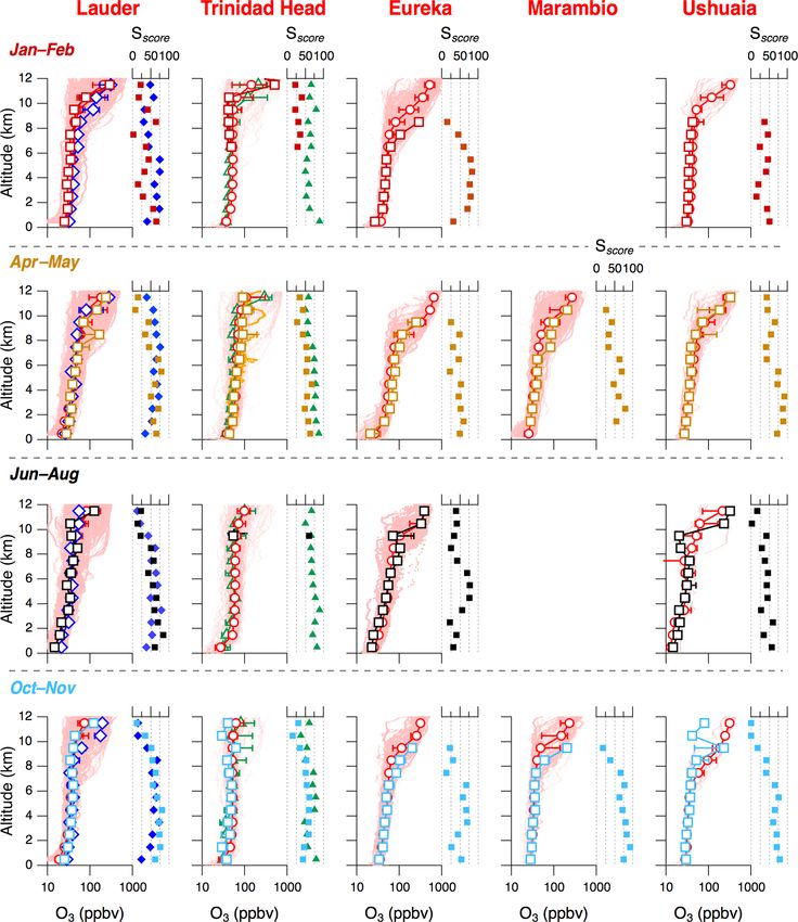
10616                                          I. Bourgeois et al.: Global-scale distribution of ozone in the remote troposphere

Figure 2. Comparison of ATom (black squares) and HIPPO (blue diamonds) monthly median O3 with ozonesonde (red circles) records from
the four tropical sites. Markers indicate the median, and the bars indicate the 25th and 75th percentiles. The three rows, from bottom to top,
correspond to the boundary layer (0–2 km), the free troposphere (2–8 km), and the UTLS (8–12 km). The pink dots show every O3 data point
measured by ozonesondes for the timeframes indicated in Table S2.

2.6    Back trajectory analysis                                          3.1    Comparison to ozonesondes

Analysis of back trajectories for air masses sampled during              ATom and HIPPO explored the fidelity with which airborne
airborne missions is useful to examine the air mass source               missions represent O3 climatology in the remote troposphere.
regions and causes of O3 variability over the Pacific and At-            Here, we show that aircraft-measured median O3 follows the
lantic oceans. We calculated 10 d back trajectories using the            seasonal ozonesonde-measured median O3 cycle at most of
TRAJ3D model (Bowman, 1993; Bowman and Carrie, 2002)                     the sites studied in this paper, as well as at almost all alti-
and National Centers for Environmental Prediction (NCEP)                 tudes – with a few exceptions (Figs. 2, 3). Figure 2 plots
global forecast system (GFS) meteorology. Trajectories were              the monthly median O3 measurements from the tropical
initialized each minute along all of the ATom flight tracks.             ozonesonde sites in three altitude bins, along with the me-
                                                                         dian values obtained from HIPPO and ATom measurements.
                                                                         Figure 3 plots the same for the extra-tropical sites. Figure 4
3     Comparison of ATom and HIPPO O3 distributions to                   correlates the median O3 measured by aircraft in Figs. 2 and
      longer-term observational records                                  3 with those measured by ozonesondes. At the Eureka site,
                                                                         the winter and spring ATom deployments recorded a sig-
Here we use existing ozonesonde and IAGOS observations
                                                                         nificantly lower median O3 compared with the correspond-
of O3 at selected locations along the ATom and HIPPO cir-
                                                                         ing ozonesonde monthly median O3 in the 0–2 km range
cuits to provide a climatological context for O3 distributions
                                                                         (Fig. 3). Eureka is frequently subject to springtime O3 deple-
derived from the systematic airborne in situ “snapshots”. We
                                                                         tion events at the surface due to atmospheric bromine chem-
quantify how much of O3 variability, occurring on timescales
                                                                         istry, which is well documented by the ozonesonde record
ranging from hours to decades, was captured by the tempo-
                                                                         (Fig. 3; Tarasick and Bottenheim, 2002). Sampling during
rally limited HIPPO and ATom missions.
                                                                         O3 depletion events significantly lowered the ATom win-
                                                                         ter and springtime O3 distributions near this site. In the 2–
                                                                         8 km range, there is a very good seasonal agreement between

Atmos. Chem. Phys., 20, 10611–10635, 2020                                                  https://doi.org/10.5194/acp-20-10611-2020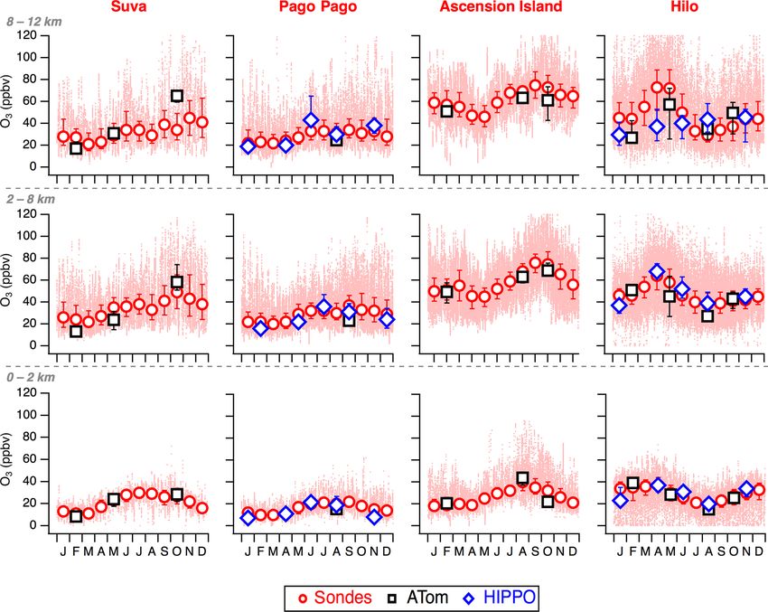
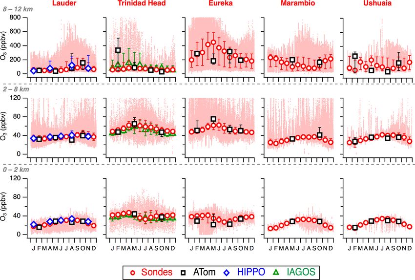
I. Bourgeois et al.: Global-scale distribution of ozone in the remote troposphere                                                10617

Figure 3. Same as in Fig. 2 but for ozonesonde launching sites located in the middle and high latitudes. O3 data obtained from the IAGOS
program (green triangles) during descents into San Francisco Bay Area airports were also added to the Trinidad Head site for comparison.

ATom/HIPPO and the ozonesondes (Fig. 4b). Most seasonal               2015a; Tarasick et al., 2019a). Furthermore, the probability
differences are found above 8 km (e.g., ATom in February              of sampling stratospheric air masses at the ATom and HIPPO
at Trinidad Head and in May at Eureka; Fig. 3) and can be             ceiling altitude (12–14 km) increases with latitude, resulting
linked to the occurrence – or absence – of stratospheric air          in a lower Sscore between the ATom/HIPPO and ozonesonde
sampling during ATom and HIPPO. In the absence of strato-             datasets at the extra-tropical sites than at the tropical sites
spheric air mixing (
10618 I. Bourgeois et al.: Global-scale distribution of ozone in the remote troposphere
3.2 Comparison to IAGOS
IAGOS O3 and CO observations in the northern Atlantic
UTLS provide a measurement-based climatology at commer-
cial aircraft cruise altitudes for comparison to ATom. Simul-
taneous measurements of O3 and CO are of particular interest
because CO provides a long-lived tracer of continental emis-
sions, which helps to differentiate O3 sources (Cohen et al.,
2018). We note that while IAGOS measurements encompass
hundreds of seasonal flights (depending on the region), ATom
sampled within each latitude band and season on one or two
flights only (Fig. 1). Thus, variability in the UT that occurred
on timescales longer than a day was not captured by ATom.
Consequently, it is not surprising to see that ATom system-
atically under-sampled tropospheric O3 (and CO) variability
compared with IAGOS at all latitudes in the northern Atlantic
(Figs. 7, 8). ATom captured on average 40 % of the O3 vari-
ability measured by IAGOS in the Atlantic UTLS (Fig. 7),
which is on par with the Sscore of 38 % obtained when com-
paring ATom and HIPPO to ozonesonde data (see Sect. 3.1).
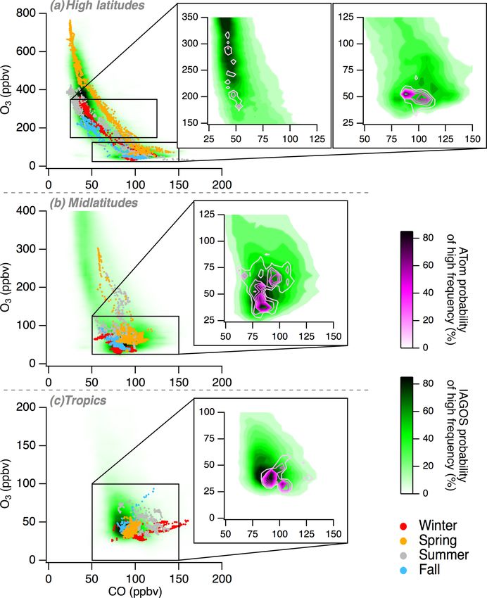
In the middle and high latitudes, the shapes of the O3 vs.
CO scatterplots from IAGOS data demonstrate that distinct
sources contribute to O3 levels in the UTLS (Fig. 8a, b;
Gaudel et al., 2015). The high O3 (>150 ppbv)–low CO
(
I. Bourgeois et al.: Global-scale distribution of ozone in the remote troposphere 10619
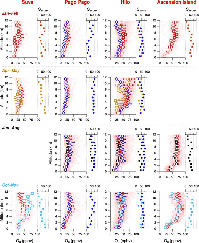
Figure 5. Seasonal comparison of 1 km vertically binned ATom (colored squares) and HIPPO (blue diamonds) median O3 with ozonesonde
(red circles) records at four sites in the tropics (Suva in Fiji, Pago Pago in American Samoa, Hilo in Hawaii, and Ascension Island). Markers
indicate the median, and the bars are the 25th and 75th percentiles. The Sscore is a metric of how well ATom and HIPPO 1 km binned O3
probability distribution functions (PDFs) overlap with the corresponding 1 km binned O3 PDFs from ozonesondes. The Sscore shown using
squares compares ATom with ozonesondes, and the Sscore shown using blue diamonds compares HIPPO with ozonesondes. The pink dots
show every O3 data point measured by ozonesondes for the timeframes indicated in Table S2.
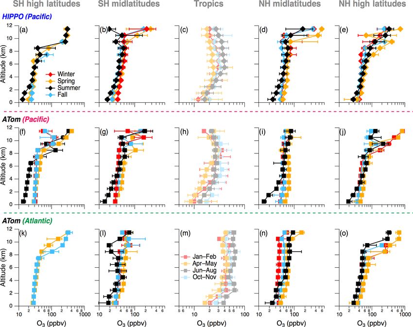
4 O3 distributions in the remote troposphere from tropospheric O3 distributions in the remote atmosphere. Fig-
ATom and HIPPO ure 9 presents the altitudinal, latitudinal, and seasonal distri-
bution of tropospheric O3 during ATom and HIPPO. Higher
We have established the fidelity of ATom and HIPPO O3 O3 was measured during ATom and HIPPO in the Northern
data by comparison to measurement-based climatologies of Hemisphere (NH) than in the Southern Hemisphere (SH),
tropospheric O3 from well-established ozonesonde and com- both in the Pacific and in the Atlantic. This distribution gra-
mercial aircraft monitoring programs. In the following sec- dient has previously been shown by global O3 mapping from
tions, we exploit the systematic nature of the ATom and modeling, satellite, and ozonesonde analyses (e.g., Hu et al.,
HIPPO vertical profiles to provide a global-scale picture of
https://doi.org/10.5194/acp-20-10611-2020 Atmos. Chem. Phys., 20, 10611–10635, 2020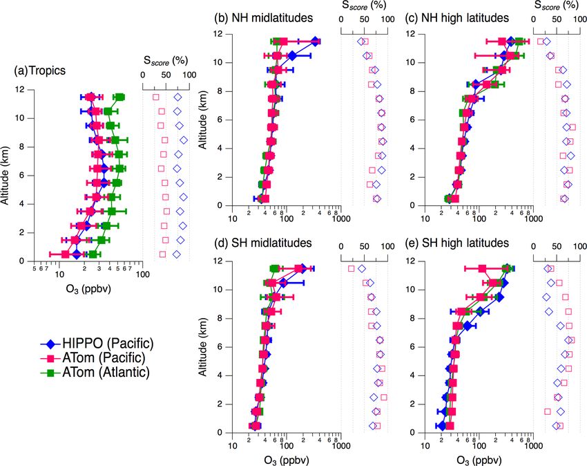
10620                                        I. Bourgeois et al.: Global-scale distribution of ozone in the remote troposphere

Figure 6. Same as in Fig. 5 but for ozonesonde launching sites located in middle and high latitudes (Lauder in New Zealand, Trinidad Head
in the USA, Eureka in Canada, Ushuaia in Argentina, and Marambio in Antarctica). O3 data obtained from the IAGOS program (green
triangles) during descents into San Francisco Bay Area airports were also added to the Trinidad Head site for comparison.

2017; Liu et al., 2013). This finding holds true throughout            ing blue diamonds, and values resulting from the comparison
the tropospheric column from 0 to 8 km, both in the middle             of ATom Atlantic and Pacific distributions are shown using
and high latitudes (Fig. S3). In the midlatitudes below 8 km,          pink squares. Figure 11 is derived from Fig. 10 and gives the
median O3 ranged between 25 and 45 ppbv in the SH and be-              Sscore values against altitude in panel (a), as well as the rela-
tween 35 and 65 ppbv in the NH. In the high latitudes below            tive difference of median O3 from 0 to 8 km in panel (b).
8 km, median O3 ranged between 30 and 45 ppbv in the SH
and between 40 and 75 ppbv in the NH. Notable features in              4.1     Tropics
the global O3 distribution are discussed in more detail in the
following sections. Figure 10 presents the vertically resolved         4.1.1    Vertical distribution
distribution of tropospheric O3 from 0 to 12 km for the At-
lantic (ATom in green) and for the Pacific (ATom in pink and           O3 is at a minimum in the tropical marine boundary layer
HIPPO in blue). Sscore values resulting from the comparison            (MBL), especially over the Pacific (Fig. 10a). The lowest
of the HIPPO and ATom Pacific distributions are shown us-              measured O3 in this region was 5.4 ppbv in May during
                                                                       ATom, and 3.5 ppbv in January during HIPPO. The tropical

Atmos. Chem. Phys., 20, 10611–10635, 2020                                                https://doi.org/10.5194/acp-20-10611-2020
I. Bourgeois et al.: Global-scale distribution of ozone in the remote troposphere 10621 Figure 7. Seasonal comparison of 1 km binned ATom (colored squares) median O3 with IAGOS (green triangles) in the northern Atlantic UTLS. Markers indicate the median, and the bars are the 25th and 75th percentiles. The three different rows indicate the latitudinal bands. The four columns indicate the seasons. The green dots show every O3 data point measured by IAGOS flights for the timeframe indicated in Table S1. MBL is a net O3 sink owing to very slow O3 production rates less than 25 ppbv below an altitude of 4 km in the tropical – NO levels averaged 22 ± 12 pptv in the Pacific and Atlantic Pacific (Fig. 10a; Oltmans et al., 2001). The relative differ- MBL during ATom – and rapid photochemical destruction ence between ATom Atlantic and Pacific median O3 in the rates of O3 in a sunny, humid environment (Kley et al., 1996; tropics below 8 km is consistently higher than a factor of 1.5, Parrish et al., 2016; Thompson et al., 1993). Deep strato- with an average Sscore of 43 % (Figs. 10a, 11b). We ascribe spheric intrusions into the Pacific MBL were not observed in this difference to O3 production from biomass burning (BB) ATom or HIPPO, in contrast to reports from previous studies emissions in the continental regions surrounding the tropi- (e.g., Cooper et al., 2005; Nath et al., 2016). In the tropics, cal Atlantic; back trajectories from the ATom flight tracks marine convection within the intertropical convergence zone show the tropical Atlantic is strongly affected by transport (ITCZ) is associated with relatively low O3 values through- from BB source regions in both Africa and South America out the tropospheric column, with median O3 mixing ratios (Fig. S4; Jensen et al., 2012; Sauvage et al., 2006; Stauffer https://doi.org/10.5194/acp-20-10611-2020 Atmos. Chem. Phys., 20, 10611–10635, 2020
10622 I. Bourgeois et al.: Global-scale distribution of ozone in the remote troposphere
4.1.2 Seasonality
The seasonal variation of vertical profiles of O3 in the trop-
ics is lower throughout the column compared with the extra-
tropics (Fig. 12), in part due to less stratospheric influence
at the highest tropical altitudes. The remoteness of the trop-
ical Pacific flight paths from continental pollution sources
also drives the lower seasonal variability here compared with
the tropical Atlantic, where the BB influence peaks in June–
August and October–November, characterized by high O3
(>75 ppbv) and high CO (>100 ppbv) (Fig. 13f), signifi-
cantly increasing the O3 vertical distribution compared with
the other seasons (Fig. 12c, h, m). Finally, photochemistry,
which regulates the O3 net balance in the troposphere, is less
seasonally variable in the tropics than in the extra-tropics,
where the photolysis frequency of O3 , j (O3 ), and the pho-
tochemical production of O3 fluctuate annually with solar
zenith angle.
4.1.3 O3 minima and maxima
Coincident O3 and CO enhancements were observed in the
tropical Atlantic for each ATom circuit (Figs. 9, 13f), sug-
gesting a year-round influence of continental emissions and
distinctive dynamics in this region (Krishnamurti et al., 1996;
Thompson et al., 1996). In the tropical Pacific, the April–
Figure 8. IAGOS and ATom seasonal O3 vs. CO scatterplots, with May period stands out due to an O3 and CO enhancement
insets showing the most frequent O3 values measured during IA- episode during HIPPO (Fig. 9) that was attributed to the
GOS and ATom. ATom seasonal deployments are colored accord- transport of anthropogenic and BB emissions from South-
ing to the legend. The frequency gradient of the O3 counts is illus- east Asia (Shen et al., 2014). Deep convection in the trop-
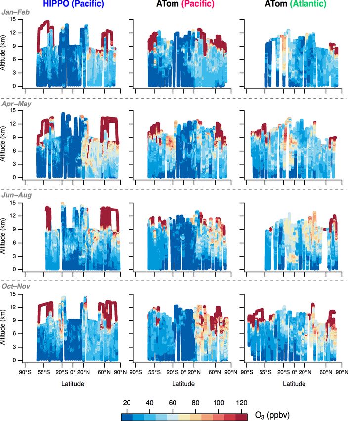
trated by the color scales (green for IAGOS and magenta for ATom). ics brings O3 -poor (I. Bourgeois et al.: Global-scale distribution of ozone in the remote troposphere 10623 Figure 9. Global-scale distribution of tropospheric O3 for each ATom and HIPPO seasonal deployment. The rows separate the seasonal deployments, whereas the columns indicate the mission and the ocean basin. The O3 color scale ranges from 20 to 120 ppbv, and all values outside of this range are shown using the same extremum color (red for values >120 ppbv and blue for values
10624                                          I. Bourgeois et al.: Global-scale distribution of ozone in the remote troposphere

Figure 10. Vertically resolved O3 distributions from 0 to 12 km are plotted for the Atlantic (ATom in green) and for the Pacific (ATom in
pink and HIPPO in blue). The five broad latitude regions correspond to the data parsing illustrated by Fig. 1. Markers indicate median O3 ,
and bars are the 25th and 75th percentiles, per 1 km altitude bin. Note the log scale on the x axis. Sscore values resulting from the comparison
of HIPPO and ATom Pacific distributions are shown using blue diamonds, and values resulting from the comparison of ATom Atlantic and
Pacific distributions are shown using pink squares.

Figure 11. All Sscore values from Fig. 10 are shown in panel (a) and are plotted against altitude. The HIPPO and ATom comparison in the
Pacific Basin is shown using blue diamonds, and a comparison of the Atlantic and Pacific basins during ATom is shown using filled pink
squares for the extra-tropics and open pink squares for the tropics. The relative difference of median O3 from 0 to 8 km given in Fig. 10 is
shown in panel (b), using the same color and marker code as in panel (a). The dotted gray lines indicate a relative difference of 20 %.

Atmos. Chem. Phys., 20, 10611–10635, 2020                                                   https://doi.org/10.5194/acp-20-10611-2020
I. Bourgeois et al.: Global-scale distribution of ozone in the remote troposphere                                                         10625

Figure 12. Seasonal variability of the regional O3 distribution in the Pacific (HIPPO in the top row and ATom in the middle row) and in the
Atlantic (ATom in the bottom row). The colors designate the local seasons with red as winter, gold as spring, black as summer, and blue as
fall (the corresponding months are indicated for the tropics, using lighter colors). The markers and associated bars correspond to the median,
25th and 75th percentiles, respectively, of the O3 distribution in every 1 km altitude bin. Note the logarithmic scale on the x axes in all panels
and the changing scale with latitudinal bin.

rapid zonal transport to smooth out variations in baseline                 different picture of O3 longitudinal distribution away from
O3 distribution in the remote troposphere, across a relatively             regional precursor emissions.
wide range of longitudes (Fig. 10b–e). The comparison of
O3 seasonal cycles at remote ozonesonde launching sites of                 4.2.2    Seasonality
the northern midlatitudes yields similar results and further
supports this conclusion (Logan, 1985; Parrish et al., 2020).
                                                                           The extra-tropical vertical profiles of O3 vary seasonally dur-
However, the similarity of the O3 distribution in the extra-
                                                                           ing ATom and HIPPO. The summer season in the middle and
tropical free troposphere above the Atlantic and Pacific is
                                                                           high latitudes was remarkable over both oceans and hemi-
not always evident in satellite-, modeling-, or ozonesonde-
                                                                           spheres for the steep O3 gradients in the tropospheric column
derived maps (Gaudel et al., 2018; Hu et al., 2017; Ziemke
                                                                           (Fig. 12 in black). In the MBL, median O3 was consistently
et al., 2017). Additionally, studies of the spatial representa-
                                                                           under 25 ppbv in the summer, whereas O3 was over 25 ppbv
tiveness of tropospheric O3 monitoring networks have also
                                                                           in other seasons. Low O3 in the MBL in summer reflects the
concluded that tropospheric O3 distributions varied signifi-
                                                                           enhanced O3 photochemical destruction in this NOx -limited
cantly with longitude, especially in the northern middle and
                                                                           region. Photochemical destruction decreases in dry air in the
high latitudes over continents (Liu et al., 2013; Tilmes et al.,
                                                                           upper troposphere, leading to the steep O3 gradients observed
2012). In contrast, the ATom findings stem from O3 measure-
                                                                           in this region. The summer O3 minimum was especially ap-
ments predominantly over the oceans, which likely reveal a
                                                                           parent in the high latitudes of the southern Pacific during

https://doi.org/10.5194/acp-20-10611-2020                                                   Atmos. Chem. Phys., 20, 10611–10635, 2020
10626 I. Bourgeois et al.: Global-scale distribution of ozone in the remote troposphere Figure 13. O3 vs. CO plots using combined ATom and HIPPO data. Each panel denotes a different latitudinal band in each basin. Seasonal deployments are colored according to the legend. Note the logarithmic scale on the y axes in all panels and the changing scale with latitudinal bin. ATom and extended well above the MBL into the free tro- been reported in the NH (e.g., Monks, 2000) when meteorol- posphere (Fig. 12 in black). O3 mixing ratios were highest ogy favors efficient transport of O3 and precursors from con- in the tropospheric column during springtime in both hemi- tinental air from North America and Eurasia (Owen et al., spheres, and over both oceans (Fig. 12 in gold). A notable 2006; Zhang et al., 2017, 2008). Another contributing fac- exception occurred during springtime in the high latitudes of tor is the increased frequency of stratospheric air mixing in the NH, where several O3 depletion events were sampled in spring that significantly contributes to higher O3 levels (Lin the lower legs of the Arctic transit. During these events, O3 et al., 2015a; Tarasick et al., 2019a). Further, the tropospheric mixing ratios lower than 10 ppbv were measured, resulting O3 springtime maximum in the SH is often attributed to BB in a lower 25th percentile of the O3 distribution at the low- emissions reaching a peak (Fishman et al., 1991; Gaudel et est altitude compared with the other seasons (Fig. 12e and o al., 2018), but stratospheric air mixing also occurs (Diab et in gold). A tropospheric O3 springtime maximum has often al., 1996, 2004; Greenslade et al., 2017). Here, the O3 −CO Atmos. Chem. Phys., 20, 10611–10635, 2020 https://doi.org/10.5194/acp-20-10611-2020
I. Bourgeois et al.: Global-scale distribution of ozone in the remote troposphere                                             10627

relationship in spring shows that the enhanced stratospheric         5   Conclusions
mixing with tropospheric air during this season, both in the
northern and southern middle and high latitudes, contributes         We present tropospheric O3 distributions measured over re-
to the increase in column O3 (Fig. 13). Fall and winter sea-         mote regions of the Pacific and Atlantic oceans during two
sons shared similar features in the middle and high latitudes:       airborne chemical sampling projects: the four deployments
no strong O3 gradient was measured in the free troposphere,          of ATom (2016–2018) and the five deployments of HIPPO
and O3 values varied over similar ranges – about 40 ppbv in          (2009–2011). The data highlight several regional- and large-
the NH and about 30 ppbv in the SH – during the two seasons          scale features of O3 distributions and provide insight into
(Fig. 12 in red and blue).                                           current O3 distributions in remote regions. The main findings
                                                                     are as follows:
4.2.3   O3 enhancements                                                 ATom and HIPPO provide a unique perspective on verti-
                                                                     cally resolved global baseline O3 distributions over the Pa-
The linear increase of O3 with CO >100 ppbv highlights the           cific and Atlantic basins and expand upon spatially limited
contribution of natural and anthropogenic pollution plumes           O3 climatologies from long-term datasets to highlight large-
lofted from continental areas into the remote troposphere. In        scale features necessary for model output and satellite re-
the NH, these events occur almost year-round (Fig. 13b–c             trieval validation.
and g–h). Higher CO enhancements in the Pacific (Fig. 13g–              ATom and HIPPO O3 data are consistent – where they
h) than in the Atlantic (Fig. 13b–c) have been observed be-          overlap – with measurement-based climatologies of tropo-
fore and have been attributed to sampling bias (Clark et al.,        spheric O3 from well-established ozonesonde and commer-
2015). Here, our findings suggest a year-round influence of          cial aircraft monitoring programs. ATom and HIPPO sea-
continental emissions on the Pacific atmosphere despite its          sonal median O3 correlated well with corresponding sea-
remoteness. Modeled back trajectories show that most air             sonal median O3 from ozonesondes (R 2 >0.7), giving con-
masses sampled in the NH during ATom were influenced                 fidence in the accurate depiction of the emerging global O3
by long-range transport of continental emissions from Asia,          climatology by these diverse research activities. ATom and
Africa, and North America (Fig. S6). Previous studies have           HIPPO captured 30 %–71 % of O3 variability measured by
shown that anthropogenic and BB emission outflow from                ozonesondes launched in the vicinity of the aircraft flight
Asia significantly contributed to O3 pollution events mea-           tracks and had the same mode of the O3 distribution as de-
sured over the northern Pacific or in California (e.g., Heald et     termined by IAGOS in the northern Atlantic UTLS. This
al., 2003; Jaffe et al., 2004; Lin et al., 2017). Intercontinental   representativeness evaluation on global scales highlights the
transport of anthropogenic emissions from Europe can also            usefulness of airborne observations to fill in the gaps of es-
contribute to the Asian outflow of anthropogenic pollution           tablished but limited O3 climatologies. Higher O3 loading in
(e.g., Bey et al., 2001; Liu et al., 2002; Newell and Evans,         the NH compared with the SH is consistent with the hetero-
2000). Finally, O3 enhancements in the northern Atlantic             geneous distribution of O3 precursor emissions around the
have frequently been observed and have been attributed to            globe, mostly concentrated in the NH, which is a result con-
midlatitude anthropogenic and boreal forest fire emissions           sistent with previous modeling studies and satellite observa-
(e.g., Honrath et al., 2004; Martín et al., 2006; Trickl et al.,     tions. ATom Atlantic vs. Pacific comparison reveals a sim-
2003). In the SH, polluted air is encountered more often in          ilar O3 distribution in the free troposphere up to ∼ 8 km in
spring and summer over the Atlantic, but springtime CO is            the middle and high latitudes, but not in the tropics. Sim-
greater than in other seasons over the Pacific (Fig. 13d–e and       ilar O3 distributions across latitude bands have been sug-
i–j). During spring, median O3 above 50 ppbv was measured            gested in the past, but these studies were limited to the north-
throughout the free troposphere in the southern midlatitudes         ern midlatitudes. Conversely, other satellite, modeling, and
(Fig. 12). Several air masses intercepted during these flights       observation-based studies indicated significant O3 longitudi-
originated from regions that were intensively burning at the         nal gradients. Here, our findings are consistent with zonal
time, notably equatorial and southern Africa, Australia, and         transport smoothing the baseline O3 distribution longitudi-
southern South America, contributing to the observed en-             nally from the Pacific to the Atlantic. In the tropics, median
hanced O3 and CO (Fig. S4). Our results expand on previous           O3 mixing ratios are about twice as high in the Atlantic as
observation-based but more spatially and temporally limited          in the Pacific, due to a well-documented mixture of dynam-
studies that highlighted co-located enhancements of O3 and           ical patterns interacting with the transport of continental air
CO at remote locations to show in situ evidence of the fre-          masses.
quent, large-scale influence of continental outflow on O3 in            A comparison of seasonal O3 vertical profiles did not re-
the remote troposphere in both oceans, as well as at almost          veal a marked seasonality in the tropics but instead high-
all latitudes.                                                       lighted the influence of specific events, most notably BB
                                                                     emissions from Africa and South America, which have been
                                                                     extensively documented in the literature. In the extra-tropics,
                                                                     the summer season was characterized by a steeper tropo-

https://doi.org/10.5194/acp-20-10611-2020                                          Atmos. Chem. Phys., 20, 10611–10635, 2020
10628 I. Bourgeois et al.: Global-scale distribution of ozone in the remote troposphere
spheric O3 gradient driven by a very low O3 abundance in the Author contributions. SCW and TBR designed the research (ATom
MBL. Fall and winter seasons generally led to near-constant and HIPPO). The measurements were carried out by IB, JP, CRT,
O3 mixing ratios from the surface to the upper troposphere, TC, RC, BD, GWD, JWE, RSG, EJH, KM, FLM, CS, and TBR.
while the highest O3 abundance was recorded during the BJJ, RK, RQ, RS, DWT, AMT, and JCW provided the ozonesonde
spring season when more frequent and intense stratospheric measurements. HC, AG, and VT provided the IAGOS measure-
ments. Back trajectory calculations were provided by ER and KCA.
intrusions and transport of air masses from continental re-
IB, JP, CRT, KCA, RC, AG, EJH, KM, DDP, RQ, ER, DWT, AMT,
gions occur. ATom and HIPPO provide the first airborne in VT, JCW, SCW, and TBR contributed to the discussion and inter-
situ vertically resolved O3 climatology covering both the At- pretation of the results. IB, JP, and TBR wrote the paper.
lantic and Pacific oceans in the NH and in the SH. They con-
firm and extend the current understanding of O3 variability
in the remote troposphere, built over several decades by air- Competing interests. The authors declare that they have no conflict
borne campaigns, monitoring networks, and satellite obser- of interest.
vations.
Overall, this paper highlights the value of the ATom and
HIPPO datasets, which cover spatial scales commensurate Acknowledgements. We thank the ATom leadership team, the sci-
with the grid resolution of current Earth system models and ence team, and the DC-8 pilots and crew for contributions to the
are also useful as a priori estimates for improved retrievals ATom measurements. We thank Andy Neuman, Hélène Angot, and
of tropospheric O3 from satellite remote sensing platforms. Owen Cooper for helpful discussions and careful editing of this pa-
In addition, ATom and HIPPO in situ measurements help per.
to establish the quantitative legacy of global pollution trans-
port and chemistry through the evaluation of key, covarying
species – in this case O3 and CO, and reveal the year-round Financial support. ATom was funded in response to NASA
ROSES-2013 NRA NNH13ZDA001N-EVS2. The HIPPO program
pervasive influence of continental outflow on O3 enhance-
was supported by NSF grants (grant nos. ATM-0628575, ATM-
ments in the remote troposphere. ATom and HIPPO datasets 0628519, and ATM-0628388). The authors acknowledge support
should be critical for improving the scientific community’s from the U.S. National Oceanic and Atmospheric Administra-
understanding of O3 production and loss processes as well tion (NOAA) Health of the Atmosphere and Atmospheric Chem-
as the influence of anthropogenic emissions on baseline O3 istry, Carbon Cycle, and Climate programs. SHADOZ ozoneson-
in remote regions. They provide a timely addition to the Tro- des are supported by the NASA Upper Atmosphere Research pro-
pospheric Ozone Assessment Report (TOAR) effort to char- gram. Ozone soundings at Marambio have been supported by the
acterize the global-scale O3 distribution and address some of Finnish Antarctic research program (FINNARP). The IAGOS pro-
the measurement gaps identified therein. gram acknowledges the European Commission for its support of
the MOZAIC project (1994–2003), the preparatory phase of IA-
GOS (2005–2013), and IGAS (2013–2016); the partner institutions
Data availability. ATom data can be obtained from the ATom of the IAGOS Research Infrastructure (FZJ, DLR, MPI, and KIT
data repository at the NASA/ORNL DAAC: https://doi.org/10. in Germany; CNRS, Météo-France, and Université Paul Sabatier in
3334/ORNLDAAC/1581 (Wofsy et al., 2018). HIPPO data can France; and the University of Manchester in the UK); the French
be obtained from the HIPPO data repository at the NCAR/EOL Atmospheric Data Center AERIS for hosting the database; and the
data archive https://doi.org/10.3334/CDIAC/HIPPO_010 (Wofsy participating airlines (Lufthansa, Air France, China Airlines, Iberia,
et al., 2017). IAGOS datasets were obtained from the ex- Cathay Pacific, and Hawaiian Airlines) for transporting the instru-
isting MOZAIC-IAGOS database and are freely available on mentation free of charge.
http://www.iagos.fr (last access: 15 January 2019) or via the
AERIS web site http://www.aeris-data.fr (last access: 15 Jan-
uary 2019). Ozonesonde measurements are all freely accessi- Review statement. This paper was edited by Hang Su and reviewed
ble and are provided by the WMO/GAW Ozone Monitoring by two anonymous referees.
Community, World Meteorological Organization–Global Atmo-
sphere Watch Program (WMO-GAW)/World Ozone and Ultra-
violet Radiation Data Centre (WOUDC) at https://woudc.org
(https://doi.org/10.14287/10000001; last access: 15 January 2019). References
A list of all contributors to ozonesonde measurements is available
on the WOUDC website. Andreae, M. O., Anderson, B. E., Blake, D. R., Bradshaw,
J. D., Collins, J. E., Gregory, G. L., Sachse, G. W., and
Shipham, M. C.: Influence of plumes from biomass burn-
Supplement. The supplement related to this article is available on- ing on atmospheric chemistry over the equatorial and tropical
line at: https://doi.org/10.5194/acp-20-10611-2020-supplement. South Atlantic during CITE 3, J. Geophys. Res., 99, 12793,
https://doi.org/10.1029/94JD00263, 1994.
Bey, I., Jacob, D. J., Logan, J. A., and Yantosca, R. M.: Asian
chemical outflow to the Pacific in spring: Origins, pathways,
Atmos. Chem. Phys., 20, 10611–10635, 2020 https://doi.org/10.5194/acp-20-10611-2020You can also read