Global and regional impacts of land cover changes on isoprene emissions derived from spaceborne data and the MEGAN model
←
→
Page content transcription
If your browser does not render page correctly, please read the page content below
Atmos. Chem. Phys., 21, 8413–8436, 2021
https://doi.org/10.5194/acp-21-8413-2021
© Author(s) 2021. This work is distributed under
the Creative Commons Attribution 4.0 License.

Global and regional impacts of land cover changes on isoprene
emissions derived from spaceborne data and the MEGAN model
Beata Opacka1 , Jean-François Müller1 , Trissevgeni Stavrakou1 , Maite Bauwens1 , Katerina Sindelarova2 ,
Jana Markova2,3 , and Alex B. Guenther4
1 Royal Belgian Institute for Space Aeronomy (BIRA-IASB), Avenue Circulaire 3, 1180 Brussels, Belgium
2 Department of Atmospheric Physics, Charles University in Prague, Prague, Czech Republic
3 Czech Hydrometeorological Institute (CHMI), Na Šabatce 17, 14306, Prague 4, Czech Republic
4 Department of Earth System Science, University of California Irvine, 92697, California, USA

Correspondence: Beata Opacka (beata.opacka@aeronomie.be) and Jean-François Müller (jfm@aeronomie.be)

Received: 1 February 2021 – Discussion started: 12 February 2021
Revised: 30 April 2021 – Accepted: 3 May 2021 – Published: 3 June 2021

Abstract. Among the biogenic volatile organic compounds            suses, clear cut areas and seedling or young trees are clas-
(BVOCs) emitted by plant foliage, isoprene is by far the           sified as forest, while satellite-based mappings of trees rely
most important in terms of both global emission and atmo-          on a minimum height. Three inventories of isoprene emis-
spheric impact. It is highly reactive in the air, and its degra-   sions are generated, differing only in their LULC datasets
dation favours the generation of ozone (in the presence of         used as input: (i) the static distribution of the stand-alone ver-
NOx ) and secondary organic aerosols. A critical aspect of         sion of MEGAN, (ii) the time-dependent MODIS land cover
BVOC emission modelling is the representation of land use          dataset, and (iii) the MODIS dataset modified to match the
and land cover (LULC). The current emission inventories are        tree cover distribution from the GFW database. The mean
usually based on land cover maps that are either modelled          annual isoprene emissions (350–520 Tg yr−1 ) span a wide
and dynamic or satellite-based and static. In this study, we       range due to differences in tree distributions, especially in
use the state-of-the-art Model of Emissions of Gases and           isoprene-rich regions. The impact of LULC changes is a mit-
Aerosols from Nature (MEGAN) model coupled with the                igating effect ranging from 0.04 to 0.33 % yr−1 on the pos-
canopy model MOHYCAN (Model for Hydrocarbon emis-                  itive trends (0.94 % yr−1 ) mainly driven by temperature and
sions by the CANopy) to generate and evaluate emission in-         solar radiation. This study highlights the uncertainty in spa-
ventories relying on satellite-based LULC maps at annual           tial distributions of and temporal variability in isoprene asso-
time steps. To this purpose, we first intercompare the dis-        ciated with remotely sensed LULC datasets. The interannual
tribution and evolution (2001–2016) of tree coverage from          variability in the emissions is evaluated against spaceborne
three global satellite-based datasets, MODerate resolution         observations of formaldehyde (HCHO), a major isoprene ox-
Imaging Spectroradiometer (MODIS), ESA Climate Change              idation product, through simulations using the global chem-
Initiative Land Cover (ESA CCI-LC), and the Global For-            istry transport model (CTM) IMAGESv2. A high correlation
est Watch (GFW), and from national inventories. Substantial        (R > 0.8) is found between the observed and simulated in-
differences are found between the datasets; e.g. the global        terannual variability in HCHO columns in most forested re-
areal coverage of trees ranges from 30 to 50 × 106 km2 , with      gions. The implementation of LULC change has little impact
trends spanning from −0.26 to +0.03 % yr−1 between 2001            on this correlation due to the dominance of meteorology as
and 2016. At the national level, the increasing trends in for-     a driver of short-term interannual variability. Nevertheless,
est cover reported by some national inventories (in particular     the simulation accounting for the large tree cover declines
for the US) are contradicted by all remotely sensed datasets.      of the GFW database over several regions, notably Indone-
To a great extent, these discrepancies stem from the plurality     sia and Mato Grosso in Brazil, provides the best agreement
of definitions of forest used. According to some local cen-        with the HCHO column trends observed by the Ozone Mon-

Published by Copernicus Publications on behalf of the European Geosciences Union.
8414                                                  B. Opacka et al.: Impacts of land cover changes on isoprene emissions

itoring Instrument (OMI). Overall, our study indicates that        nity Land Model (CLM; Lawrence et al., 2019). However,
the continuous tree cover fields at fine resolution provided       human-driven land use practices must be included from other
by the GFW database are our preferred choice for constrain-        independent datasets of crops from Ramankutty and Foley
ing LULC (in combination with discrete LULC maps such              (1999) or from De Noblet-Ducoudré and Peterschmitt used
as those of MODIS) in biogenic isoprene emission models.           in Lathière et al. (2010), the 1500–2100 land use dataset from
                                                                   Hurtt et al. (2011), or the 2015–2100 GCAM-Demeter land
                                                                   use dataset from Chen et al. (2020). The evaluation of the
                                                                   present-day impact of LULCC on BVOC emissions could
1   Introduction                                                   however benefit from the availability of satellite observa-
                                                                   tions. Remotely sensed land cover (LC) maps are built with
The total biogenic volatile organic compound (BVOC) emis-          either discrete classification schemes, the result of which is
sion into the atmosphere amounts to ca. 1000 Tg yr−1 of            a raster (e.g. ESA Climate Change Initiative Land Cover –
which about 50 %–60 % of the share consists of isoprene            ESA CCI-LC – and MODerate resolution Imaging Spectro-
(Lathière et al., 2006; Guenther et al., 2012; Sindelarova         radiometer – MODIS – MCD12Q1 and MCD12C1), or as
et al., 2014; Messina et al., 2016; Granier et al., 2019) and      continuous classification, viewing vegetation as a continuum,
is roughly equal to the global methane emission (Lelieveld         obtained with the use of vegetation spectral indices (e.g.
et al., 1998; Saunois et al., 2020). Isoprene is highly reactive   MODIS VCF MOD44B; AVHRR VCF VCF5KYR; Sexton
and affects tropospheric chemistry (Fehsenfeld et al. 1992;        et al., 2013; Hansen et al., 2013). Traditionally, LC products
Atkinson, 2000; Pike and Young, 2009). Under high-NOx              use a discrete biome-based classification approach. The main
conditions (NOx ≡ NO + NO2 ), isoprene is a major precur-          drawback is that biomes are not natural vegetation units with
sor of tropospheric ozone (Atkinson, 2000; Ryerson et al.,         common physiological and biochemical features required in
2001; da Silva et al., 2018; Mo et al., 2018; Saunier et al.,      the land surface modelling but are products of classifica-
2020). BVOCs also affect the growth of secondary organic           tion. Plant functional types, or PFTs, commonly adopted in
aerosols (Claeys et al., 2004; Kroll et al., 2005, 2006; Carl-     modelling, comprise plant species that share similar plant
ton et al., 2009) and influence tropospheric hydroxyl radi-        physiognomy (tree, shrub, or grass), leaves (needleleaf or
cal (OH) levels through depletion or regeneration (Lelieveld       broadleaf), phenology (evergreen or deciduous), and photo-
et al., 2008; Hofzumahaus et al., 2009; Fuchs et al., 2013;        synthetic types (C3 or C4 ) for crops and grasses (Smith et al.,
Hansen et al., 2017), thereby altering the lifetime of methane.    1997; Bonan et al., 2002). Currently, PFT classifications are
Isoprene is primarily emitted from terrestrial vegetation, in      obtained through the mapping from biome schemes, a com-
particular broadleaf trees, and therefore, isoprene emissions      plex task that is flawed by arbitrariness (Bonan et al., 2002;
are critically dependent on the land cover (e.g. tree, shrub,      Sun and Liang, 2008; Ustin and Gamon, 2010; Poulter et al.,
grass, crop) and on the plant species within those land covers     2015).
(Arneth et al., 2011; Guenther et al., 2012).                         The present study aims to incorporate different satellite-
   Land use and land cover changes (LULCCs) are consid-            based land cover datasets in the Model of Emissions of Gases
ered among the main drivers of environmental and climate           and Aerosols from Nature (MEGAN) model (Guenther et al.,
changes (Foley et al., 2005; Turner et al., 2007; Jia et al.,      2006, 2012) for estimating global isoprene emissions and to
2019). They bring about disruption in land–atmosphere in-          give a measure of the uncertainty associated with their use.
teractions through multiple biophysical and biogeochemical         It complements the study of Chen et al. (2018) about the im-
fluxes across different spatial and temporal scales. In par-       pact of LULCCs on isoprene emissions based on remotely
ticular, the impact of deforestation on the climate system         sensed LC. The methodology is presented in Sect. 2. Sec-
was reviewed by Bonan (2008), Unger (2014), Scott et al.           tion 3 reviews the distribution and trends of tree cover (TC)
(2018), and Zeppetello et al. (2020). Distribution and dis-        through 2001–2016 at regional and global scales from differ-
turbances in vegetation, in particular trees, have an impact       ent satellite-based LC products. A comparison with the latest
on the emissions of BVOCs that in turn control the load-           2020 database from Forest Resources Assessment (FRA) is
ings of several short-lived climate forcers, with effects on       made, and trends over large forested regions are discussed.
climate via the radiative forcing (Unger, 2014; Ward et al.,       In Sect. 4, we perform a sensitivity analysis and quantify the
2014) and over the long-term via the climate–carbon feed-          impact of LULCCs on estimated isoprene emissions using
back (Fu et al., 2020). The effect of historical or projected      MEGAN-MOHYCAN (Model for Hydrocarbon emissions
LULCCs on BVOC emissions were reviewed, for instance,              by the CANopy; Guenther et al., 2012; Müller et al., 2008).
in Peñuelas and Staudt (2010), Unger (2013, 2014), and             In Sect. 5, the IMAGESv2 global chemistry transport model
Hantson et al. (2017). Estimates of past and future emis-          (CTM) with BVOC emissions obtained in Sect. 4 is used
sions accounting for climate change and increasing CO2 lev-        to evaluate the simulated interannual variability and trends
els rely on dynamic global vegetation models such as OR-           in formaldehyde (HCHO) columns between 2005 and 2016
CHIDEE (Krinner et al., 2005), LPJ-GUESS (Sitch et al.,            against satellite observations from the Ozone Monitoring In-
2003), SDGVM (Woodward and Lomas, 2004), or Commu-                 strument (OMI). While direct satellite observations of iso-

Atmos. Chem. Phys., 21, 8413–8436, 2021                                              https://doi.org/10.5194/acp-21-8413-2021
B. Opacka et al.: Impacts of land cover changes on isoprene emissions                                                         8415

prene are still in the early stages of development (Fu et al.,      sume that the foliage covers only the vegetated fraction of the
2019; Wells et al., 2020), the evaluation method used here          grid cell. The stand-alone MEGANv2.1 uses a static vegeta-
is based on spaceborne formaldehyde (HCHO) and relies on            tion map that provides the spatial distribution of 16 PFTs for
the fact that HCHO is a high-yield product of the oxidation         the present day compatible with the Community Land Model
of isoprene and has been widely used in past studies (Palmer        version 4 (CLM4; Lawrence and Chase, 2007; Lawrence
et al., 2006; Millet et al., 2008; Stavrakou et al., 2009; Marais   et al., 2011) including trees, shrubs, and grasses (Table S1
et al., 2012; Bauwens et al., 2016; Kaiser et al., 2018). Con-      in the Supplement). In each model grid, vegetation is de-
clusions are drawn in Sect. 6.                                      fined by the fractional coverage of each of the PFTs. This
                                                                    PFT distribution was based on various satellite products from
                                                                    MODIS, AVHRR, and the global cropland distribution for
2     Methods: datasets and model descriptions                      the year 2000 from Ramankutty et al. (2008), and hereafter, it
                                                                    is referred to as CLM. The methodology is briefly described
2.1    MEGAN-MOHYCAN: biogenic VOC emission
                                                                    in Oleson et al. (2010). The emission factor ε is calculated
       modelling
                                                                    based on PFT-dependent emission factors provided in Guen-
The biogenic emissions of isoprene, monoterpenes, and 2-            ther et al. (2012) weighted by the fractional areal coverage of
methylbutenol are estimated using the Model of Emissions            the corresponding PFT class of a grid cell (Table S1).
of Gases and Aerosols from Nature (MEGAN; Guenther
et al., 2006, 2012) coupled with the Model for Hydro-               2.2     Satellite-based vegetation datasets
carbon emissions by the CANopy (MOHYCAN; Wallens,
2004; Müller et al., 2008), a multi-layer canopy environ-           The current satellite-based LC products cannot be directly
ment model. MEGAN estimates the net emission rates F                translated into PFT classes for use in MEGAN-MOHYCAN
(µg m−2 h−1 ) into the above-canopy atmosphere using simple         since they differ by their primary classification, traditionally
mechanistic algorithms encapsulated in the following equa-          biome-based, and by the number of classes (Sun and Liang,
tion:                                                               2008). In order to generate MEGAN-compatible LC maps,
                                                                    the biome classes were first cross-walked (reclassified) into
F =  · γ,    with γ = CCE · γPT · LAI · γA · γCO2 · γSM , (1)      phenology-based PFT classes. The uncertainty of this step is
                                                                    mainly due to the relative arbitrariness of the cross-walking
where the emission factor ε (µg m−2 h−1 ) represents the            land cover legend tables resulting from the sometimes am-
emission rate at standard conditions. The latter specify all        biguous definitions of the biome classes. Next, the PFT trees
relevant meteorological (temperature, solar radiation, air hu-      and shrubs were further subdivided into zonal or geograph-
midity, soil moisture, wind speed, etc.) and phenological           ical subtypes (tropical, temperate, and boreal), and grasses
(leaf area index, LAI, and leaf age, A) variables, as defined       were subdivided into photosynthetic pathways C3 and C4 ,
by Guenther et al. (2006). Deviations from those conditions         based on the Köppen–Geiger maps and climatological con-
are accounted for by the activity factors γ representing the        siderations, as explained in the following section.
response of biogenic emissions to their major identified en-           Three datasets were considered that provide global-scale
vironmental and phenological drivers such as leaf tempera-          time-dependent vegetation maps over 2001–2016 (Tables 1
ture (T ), photosynthetic photon flux density (P ), soil mois-      and 2). Those include the land cover maps based on biome
ture (SM), CO2 concentration, A, and LAI. The temperature           classes from (1) the MODerate resolution Imaging Spectro-
and light response algorithm incorporates the influence of          radiometer (MODIS), (2) the European Space Agency (ESA)
the past conditions. The adjustment factor CCE related to the       Climate Change Initiative Land Cover (CCI LC), and (3) the
canopy environment model is set to 0.52 for MOHYCAN                 tree cover product of the Global Forest Watch (GFW; Hansen
so that γ = 1 at standard canopy conditions. The effects of         et al., 2013) based on 30 m Landsat images. The schematic
CO2 inhibition and soil moisture stress are neglected here          representation of the consecutive transformations applied on
(γCO2 = 1 and γSM = 1).                                             the original datasets is shown in Fig. S1 in the Supplement.
   The meteorological fields are obtained from ECMWF
(European Centre for Medium-Range Weather Forecasts)                2.2.1    Köppen–Geiger biome types
Interim reanalysis (ERA-Interim; Dee et al., 2011). The
canopy model determines the leaf temperature and the ra-            The subdivisions of climate zones and C3 /C4 photosynthetic
diation fluxes as a function of height inside the canopy.           paths are obtained based on Table 3 from Poulter et al.
The land cover features are described by the LAI and the            (2011) that establishes a simplified correspondence between
vegetation map, classified as PFTs. Monthly LAI distribu-           the Köppen–Geiger classes and climate zones defined on
tions at 0.5◦ × 0.5◦ resolution (in m2 m−2 ) are based on the       the basis of temperature criteria. In particular, the distinc-
MODIS dataset (MODIS 15A2H collection 6) available at               tion between C3 and C4 photosynthesis adaptations is set
https://lpdaac.usgs.gov (last access: 31 May 2021). Follow-         at the threshold temperature of 22◦ C (Collatz et al., 1998).
ing Guenther et al. (2006) and Müller et al. (2008), we as-         The methodology is described in the Supplement. The dis-

https://doi.org/10.5194/acp-21-8413-2021                                              Atmos. Chem. Phys., 21, 8413–8436, 2021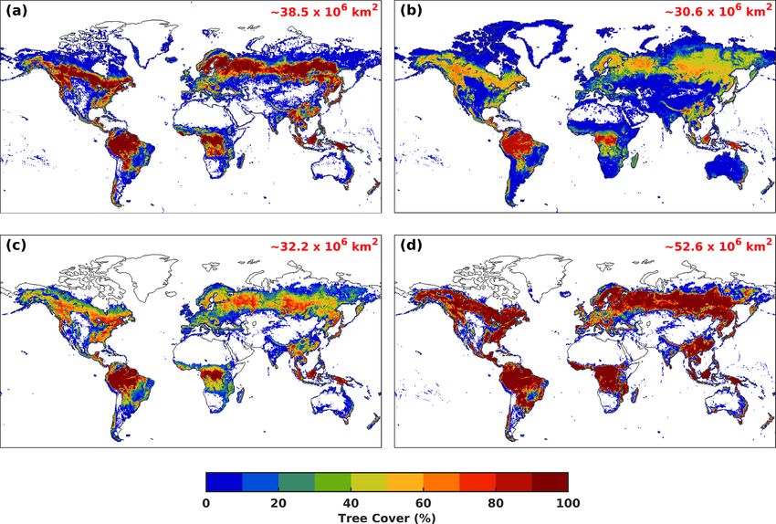
8416                                                      B. Opacka et al.: Impacts of land cover changes on isoprene emissions

Table 1. Main features of the satellite vegetation products used for the comparison of land cover maps. Discrete LULC products, namely
MCD12Q1 and ESA CCI-LC, rely on a primary classification (PC) such as the LCCS, standing for Land Cover Classification System. Details
are found in Sect. 2.2.

   Products                                Satellite sensors      Resolution     Availability
   MCD12Q1 (v006)                          MODIS Terra/Aqua       500 m          Global, gridded, annual (2001–2019)
   Friedl and Sulla-Menashe (2019)                                               https://lpdaac.usgs.gov (last access: 31 May 2021)
   Discrete LULC using LCCS as PC
   ESA CCI-LC                              AVHRR                  300 m          Global, gridded, annual (1992–2019)
   (v2.0.7 and v2.1.1)                     MERIS FR and RR                       https://maps.elie.ucl.ac.be (last access: 31 May 2021)
   ESA CCI-LC (2017)                       SPOT-VGT                              https://cds.climate.copernicus.eu        (last    access:
   Discrete LULC using LCCS as PC          PROBA-V                               31 May 2021)
   GFW (v1.6)                              Landsat and MODIS      30 m           Global, gridded, possibility to reconstruct annual up-
   Hansen et al. (2013)                                                          dates (2000–2019) based on the three datasets provided:
   Continuous TC field                                                           (i) TC for 2000; (ii) cumulative TC gain for 2000–
                                                                                 2012; (iii) tree loss for every year between 2001 and
                                                                                 2019. https://earthenginepartners.appspot.com (last ac-
                                                                                 cess: 31 May 2021)

Table 2. Land cover maps considered in this study, including their labels and the datasets on which they are based (described in Table 1).
The target period of this study is 2001–2016.

                   Short name of land cover maps used in this study      Original satellite-based products
                   CLM                                                   CLM4 PFT
                   ESA                                                   ESA CCI-LC
                   MODIS                                                 MODIS PFT (MCD12Q1)
                   GFWMOD                                                TC from Hansen et al. (2013) and MODIS PFT

Table 3. Global TC areas (in 106 km2 ) in the year 2001 and trends       2.2.2   ESA-CCI LC: land cover map
(in % yr−1 and in km2 yr−1 ) over 2001–2016 based on FAOSTAT,
the static land cover map (CLM), and the satellite products (ESA,        The ESA CCI-LC product supplies global annual land
MODIS, and GFWMOD).                                                      cover maps at 300 m resolution (ESA-CCI-LC, 2017). Maps
                                                                         were generated by combining the global daily surface re-
                    Area in 2001               Trends                    flectance of five different observation systems: Advanced
                          (106 km2 )   (% yr−1 )   (km2 yr−1 )           Very High Resolution Radiometer (AVHRR), Satellite Pour
                                                                         l’Observation de la Terre – Vegetation (SPOT-VGT), PRoject
       FAOSTAT                 41.5      −0.12       −49 727             for On-Board Autonomy – Vegetation (PROBA-V), and
       CLM                     38.5          –             –             Medium Resolution Imaging Spectrometer (MERIS) full and
       ESA                     30.6      −0.05       −13 968
                                                                         reduced resolutions (FR and RR).
       MODIS                   52.6       0.03        18 184
                                                                            The original product has 37 classes from the United Na-
       GFWMOD                  32.2      −0.26       −83 336
                                                                         tions LCCS (UN-LCCS). The cross-walking table for their
                                                                         conversion to PFTs is taken from Li et al. (2018) based on
                                                                         Poulter et al. (2015). The PFT mapping and the aggregation
tributions of biomes from the original classification of Poul-           into 0.5◦ × 0.5◦ were performed using the ESA CCI-LC user
ter et al. (2011) and the modified version thereof are listed            tool (version 4.3) available at https://maps.elie.ucl.ac.be (last
in Table S2 in the Supplement and displayed in Fig. S2 in                access: 31 May 2021). The mapping to climate zones and
the Supplement. We use the 0.5◦ × 0.5◦ resolution, global                photosynthetic paths is applied as described above. The final
Köppen–Geiger present-day (1980–2016) climate classifica-                land cover map will be referred to as ESA.
tion map from Beck et al. (2018), developed at 1 km resolu-
tion. The Köppen–Geiger maps are available at http://www.
                                                                         2.2.3   MODIS PFT: land cover map
gloh2o.org/koppen (last access: 31 May 2021).
                                                                         The collection 6 of the MODIS Land Cover Type Prod-
                                                                         uct (MCD12Q1; Friedl and Sulla-Menashe, 2019) provides

Atmos. Chem. Phys., 21, 8413–8436, 2021                                                     https://doi.org/10.5194/acp-21-8413-2021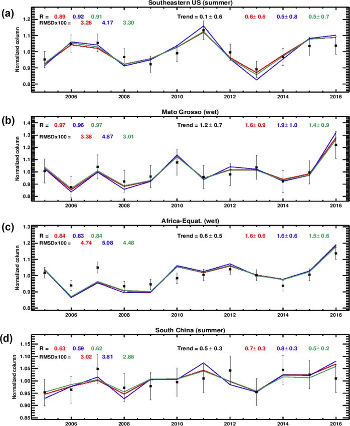
B. Opacka et al.: Impacts of land cover changes on isoprene emissions                                                       8417

a global land cover product at 500 m resolution at yearly          2.4   Formaldehyde observations from OMI
intervals from 2001 to the present. The product is derived
from the reflectance data of the Terra and Aqua missions.          Tropospheric HCHO columns are acquired from satellite-
We use here the MODIS LC product available with the PFT            based OMI observations on board the NASA AURA space-
legend. Unlike in collection 5, where 17 IGBP (Interna-            craft launched in 2004 (Levelt et al., 2006). OMI is a nadir-
tional Geosphere–Biosphere Programme) classes were cross-          viewing imaging spectrometer observing Earth’s global so-
walked to create annual maps for the PFT scheme, the UN-           lar backscatter radiation in the ultraviolet–visible spectral
LCCS (United Nations Land Cover Classification System; Di          window at a spectral resolution of about 0.5 nm. It has
Gregorio, 2005) scheme provides the primary layer for the          an early afternoon overpass time (13:30 LT) and provides
sixth collection. Note however that the corresponding cross-       global observation on a daily basis at a spatial resolution of
walking table is not released. The maps are aggregated to          13 km × 24 km at nadir.
0.5◦ × 0.5◦ , on which further subdivisions of climate zones          The OMI HCHO product used in this study was developed
and photosynthetic paths are applied following the method-         in the framework of the EU FP7 project QA4ECV (Qual-
ology described above.                                             ity Assurance for Essential Climate Variables; http://www.
                                                                   qa4ecv.eu, last access: 31 May 2021) and is documented in
2.2.4    GFW: tree cover map                                       De Smedt et al. (2015, 2017, 2018). The retrieval approach
                                                                   consists of three steps. Firstly, the HCHO slant columns are
Unlike the discrete LC maps of MODIS PFT and ESA CCI-              retrieved in the 328.5–359 nm spectral window using up-to-
LC, the Global Forest Watch dataset (Hansen et al. 2013)           date differential optical absorption spectroscopy (DOAS) al-
is a continuous field of tree cover (TC) coverage, available       gorithms (De Smedt et al., 2018) with the HCHO absorption
at a global scale with approximately 30 m resolution. In re-       cross section from Meller and Moortgat (2000). Secondly, for
cent years, it has become a reference for monitoring forests       weak absorbers such as HCHO, the background normaliza-
through the online platform Global Forest Watch (https://          tion of the slant columns using the equatorial Pacific Ocean
www.globalforestwatch.org, last access: 31 May 2021). It           as the reference sector is applied in order to compensate for
is generated by combining data from the multispectral sen-         possible systematic latitude-dependent offsets in spectral fit-
sors Landsat 5 and 7 for 2000–2012 and Landsat 8 for               ting. Eventually, the conversion into a vertical column is per-
2013 onward. The resulting images are normalized by us-            formed with the air mass factor (AMF) assuming an optically
ing MODIS surface reflectance (Hansen et al., 2008; Potapov        thin approximation. The latter is obtained from an altitude-
et al., 2012). The version 1.6 used in this study covers all       resolved AMF look-up table derived at 340 nm from the VLI-
years from 2000 to 2018 and provides tree losses on an an-         DORTv2.6 radiative transfer model (Spurr, 2008) and the
nual basis over 2000–2018 and a cumulative tree gain dis-          daily a priori vertical profile shape of the HCHO distribution
tribution over 2000–2012. We reconstructed annual steps of         calculated with the TM5-MP chemical transport model (Hui-
the TC at pixel level (30 m) by accounting for the TC losses       jnen et al., 2010; Williams et al., 2017). The scattering due
since 2000 and, by implementing the 12-year cumulative tree        to clouds is corrected using the independent pixel approxi-
cover gain at 0.5◦ resolution assuming a linear increase over      mation (Martin et al., 2002), whereas an implicit correction
the period, extended until 2018. The land cover distribution       for the effects of aerosols is accounted for through the cloud
GFWMOD (Table 2) is obtained by modifying the MODIS                correction scheme.
PFT dataset in order to match the reconstructed yearly TC
distribution based on the GFW dataset.                             2.5   The IMAGESv2 CTM

2.3     Forest Resources Assessment (FRA) database –               Simulations of the atmospheric composition are performed
        Food and Agriculture Organization (FAOSTAT)                using IMAGESv2 (Intermediate Model of the Global and
                                                                   Annual Evolution of Species), a global three-dimensional
The standard reference on global forest resources is the           CTM of the troposphere (Müller and Stavrakou, 2005;
United Nations FAO FRA published every 5 to 10 years since         Bauwens et al., 2016; Stavrakou et al., 2016, 2018). The
1948. It provides the global database of the reported statistics   model calculates the concentrations of 170 compounds in the
from national reports on forest properties. The latest recom-      global troposphere with a spin-up time of 6 months. The hor-
mendations are outlined in the FRA 2020 (http://www.fao.           izontal resolution of the model is 2◦ × 2.5◦ , while the verti-
org/3/I8661EN/i8661en.pdf, last access: 31 May 2021). Here         cal coordinate is a hybrid sigma-pressure system resolved in
we use the latest published datasets (updated in July 2020         40 unevenly spaced levels extending from the surface to the
at the time of drafting), retrieved from http://www.fao.org/       lower stratosphere (44 hPa). The model is driven by ERA-
faostat (last access: 24 August 2020), and hereafter referred      Interim meteorological fields (Dee et al., 2011). The chem-
to as FAOSTAT.                                                     ical degradation mechanism is described in Bauwens et al.
                                                                   (2016) and Stavrakou et al. (2018).

https://doi.org/10.5194/acp-21-8413-2021                                            Atmos. Chem. Phys., 21, 8413–8436, 2021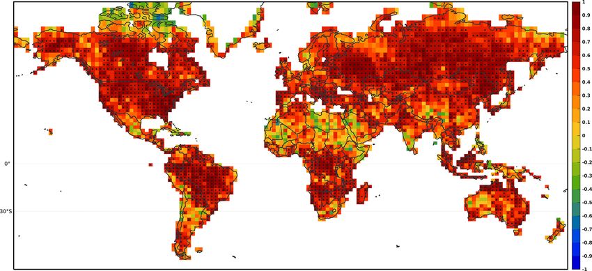
8418                                                  B. Opacka et al.: Impacts of land cover changes on isoprene emissions

   The bottom-up fluxes of HCHO precursors are prescribed          datasets, GFWMOD exhibits the strongest negative trend,
as follows. The biomass burning inventory is provided by           equal to −0.26 % yr−1 (ca. −83 500 km2 yr−1 ), which is
the Global Fire Emissions Database version 4s (GFED4s;             about 3–5 times as fast as the FAOSTAT and ESA trends
van der Werf et al., 2017) on a daily basis and a global           (Table 3). The ESA dataset shows the lowest variation (ca.
spatial resolution of 0.25◦ × 0.25◦ (https://globalfiredata.org,   −14 000 km2 yr−1 ), with a stable phase between 2004 and
last access: 31 May 2021). The anthropogenic sources of            2009. While net deforestation is found in both GFWMOD
non-methane VOC (NMVOC) species are taken from the                 and ESA datasets, the MODIS dataset exhibits a small posi-
EDGARv4.3.2 (Emission Database for Global Atmospheric              tive linear trend of ∼ 0.03 % yr−1 . The MODIS TC declines
Research; Huang et al., 2017), and the anthropogenic NOx ,         in 2001–2003 and after 2014 are more than compensated for
CO, SO2 , and NH3 are obtained from the HTAPv2 (Hemi-              by the slow increase in 2003–2014 (Fig. 2a).
spheric Transport of Air Pollution; Janssens-Maenhout et al.,         Of all biomes, tropical trees experienced the greatest net
2015) database for 2010. Due to their limited availability, the    losses according to GFWMOD and ESA datasets. This loss
EDGARv4.3.2 emissions are set constant at their 2012 val-          is 3.5 times greater in GFWMOD than in ESA (Fig. 2b and
ues after this year. Both inventories are available at https:      Table S3 in the Supplement). MODIS also presents a net de-
//edgar.jrc.ec.europa.eu (last access: 31 May 2021). The bio-      cline in tropical trees (−14 600 km2 yr−1 ), almost entirely lo-
genic emissions of isoprene, monoterpenes, and methyl-             cated in South America (Fig. 3) with little net changes over
butenol are estimated as described in Sect. 2.1. The biogenic      Africa and Southeast Asia, but it is offset by positive trends
emissions of acetaldehyde and ethanol are parameterized fol-       in the boreal and especially in the temperate domain. Un-
lowing Millet et al. (2010). Biogenic CO emissions and CO          like GFWMOD, which features a net loss in all domains,
deposition are accounted for following Müller and Stavrakou        MODIS demonstrates net gains at middle and high latitudes
(2005). Finally, the biogenic methanol emissions are pro-          of the Northern Hemisphere, with the biggest changes en-
vided by an inverse modelling study constrained by space-          countered in temperate forests (18 400 km2 yr−1 ). As a re-
borne methanol data (Stavrakou et al., 2011).                      sult, these biomes, with strong trends and covering together
                                                                   roughly 60 % of the total TC area, drive the global net in-
                                                                   crease found in the MODIS dataset. Compared to the other
3     Comparison of satellite-based tree cover datasets            two datasets, the MODIS distribution shows significant im-
                                                                   pacts over much larger areas, mainly in the periphery of
The LULC datasets shown in Table 2 are compared in detail          major forests of South America, Africa, and the southeast-
below over the 2001–2016 period, namely MODIS, GFW-                ern US. In contrast, GFWMOD displays large net changes
MOD, and ESA. In this study, the tree cover refers to the          within higher-density forest canopies like those in the trop-
aggregation of the eight PFTs corresponding to trees from          ics, the southeastern US, China, and Scandinavia. In the ESA
the CLM4 PFT classification scheme (Table S1).                     dataset, the net TC changes are sparse and weak, about 1 or-
                                                                   der of magnitude lower than in the two other satellite-based
3.1    Global TC areas, spatial distributions, and trends          products, and show the highest values in boreal and temper-
                                                                   ate regions (Fig. 3).
The global TC distributions for the year 2001 are depicted in
Fig. 1. The global TC areas provided therein and listed in Ta-     3.2     National and regional distributions of trends in
ble 3 range from 30.6 × 10⁶ km2 for ESA to 52.6 × 10⁶ km2                  large forested countries
for MODIS, with the TC areas of GFWMOD and CLM
falling in between with 32.2 and 38.5×10⁶ km2 , respectively.      The satellite-based TC trends are compared against national
MODIS TC stands out as it exhibits extensive patches of high       inventories collected through FRA national reports for sev-
TC densities (> 90 %) in all major forested regions. In con-       eral large countries in Fig. 4 and Tables S4 and S5 in the
trast, GFWMOD and ESA exhibit lower densities (40 %–               Supplement. Overall, large discrepancies are found across
80 %) in the Northern Hemisphere. The ESA cover density            the different estimates with respect to both the magnitude
reaches 90 % in the tropical forests of Central Africa, the        and the sign of trends. The regional differences are further
Amazon, Southeast Asia, and Oceania. The lowest densities          discussed based on Fig. 3.
are found in the ESA dataset, e.g. in the eastern US, the West
African coast and Indonesia.                                       3.2.1    United States of America
   Table 3 compares the global satellite-based TC with fig-
ures from FAOSTAT based on national reporting. According           The US FRA report indicates a positive trend of
to FAOSTAT, the global forest area reached 41.5 × 10⁶ km2          4500 km2 yr−1 over the period considered (2001–2016),
in 2001, which lies well within the satellite-based TC areas.      whereas the satellite-based records suggest a net declining
   Time series of global TC areas normalized to the 2001           TC area. According to GFWMOD, eastern US forests experi-
values are displayed in Fig. 2a, and total global trends           ence a net deforestation, except in parts of Louisiana, Missis-
are shown in Fig. 2b and Table S2 for 2001–2016. Of all            sippi, and Florida (Fig. 3). Both MODIS and ESA show little

Atmos. Chem. Phys., 21, 8413–8436, 2021                                              https://doi.org/10.5194/acp-21-8413-2021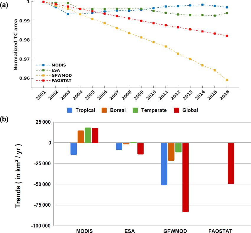
B. Opacka et al.: Impacts of land cover changes on isoprene emissions                                                              8419

Figure 1. Spatial distribution of the TC for (a) the static land cover map CLM (for the present day) and for the satellite-based datasets
((b) ESA, (c) GFWMOD, and (d) MODIS) for the year 2001. The corresponding global TC areas are provided inset.

net changes in the eastern US, except in the Mississippi Al-           tiguous to Paraguay and Caatinga, respectively (Fig. 1). The
luvial Plain. In the northwest, forests undergo deforestation          southern part of the Atlantic Forest along the eastern coast of
according to all datasets. In Alaska, GFWMOD indicates a               Brazil experiences net TC increases according to GFWMOD
clear net loss over the Yukon River Basin, also seen in the            and ESA but not MODIS.
ESA dataset although at lower rates. Overall, MODIS shows
strong positive trends in areas of low TC densities.                   3.2.3   China

3.2.2   Brazil and Indonesia                                           The strong positive trend in forest cover (∼ 22 000 km2 yr−1 )
                                                                       reported by FAOSTAT in China is not supported by any
There is qualitative agreement among all datasets regard-              space-based estimate. MODIS indicates a positive but much
ing the TC trends in Brazil and Indonesia even though                  smaller trend (+8800 km2 yr−1 ), whereas both the GFW-
there are large differences in absolute terms. Over Indone-            MOD and ESA datasets exhibit a small net loss of about
sia, the FAOSTAT trend (−4000 km2 yr−1 ) lies within the               −2500 and −350 km2 yr−1 , respectively. The spatial TC dis-
estimates based on ESA (−2550 km2 yr−1 ) and GFWMOD                    tributions reveal trends mostly in the southern part of the
(−7250 km2 yr−1 ), whereas very little changes are sug-                country. In the Yunnan–Guizhou Plateau, MODIS exhibits
gested by the MODIS dataset (−830 km2 yr−1 ). In Brazil,               net positive trends, unlike ESA and GFWMOD that show
all satellite-based estimates underestimate the national inven-        null net trends. Guangdong also experiences a net increase
tory (−32 200 km2 yr−1 ), by factors of about 2–3 in the cases         in TC according to MODIS, whereas both GFWMOD and
of GFWMOD (−16 900) and MODIS (−10 600), while ESA                     ESA indicate significant declines in southeastern China in
differs from the other satellite-based products with very low          line with the strong deforestation found in these datasets.
and sparse net total loss (−930 km2 yr−1 ). GFWMOD ex-
hibits deforestation across the Cerrado and Caatinga regions,          3.2.4   Russia
with the border regions of the Amazon forest and Cerrado ex-
periencing the largest net losses. In MODIS, strong positive           Over Russia, FAOSTAT and MODIS record total net increas-
and negative trends are found in areas of low TC density con-          ing trends of 4000 and 9300 km2 yr−1 , respectively, while the

https://doi.org/10.5194/acp-21-8413-2021                                                 Atmos. Chem. Phys., 21, 8413–8436, 2021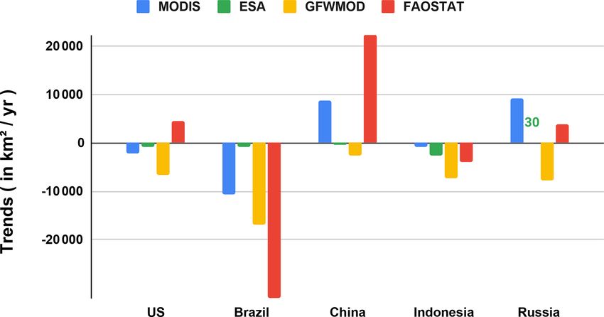
8420                                                    B. Opacka et al.: Impacts of land cover changes on isoprene emissions

Figure 2. TC trends over 2001–2016. (a) Time series of the global net changes in TC areas (normalized to 2001 values) from FAOSTAT,
MODIS, ESA, and GFWMOD datasets and (b) total net TC trends at global scale and per climate zone (as defined in Sect. 2 in the Supplement
and depicted in Fig. S2b). For the FAOSTAT dataset, TC trends per climate zone are not available.

trend is negligible for ESA, and GFWMOD presents a net                 higher than 5 m are classified as trees. A forest cover is de-
negative trend, ca. −7700 km2 yr−1 . All satellite-based trend         rived from the tree cover by applying a minimum threshold
distributions (Fig. 3) exhibit net positive trends in a large          for the canopy cover and integrating over entire pixel areas
zone around 55◦ N between Belarus and the West Siberian                where the condition is met. Table 4 summarizes the criteria
Plains. In the Central Siberian Plateau, the strongest net pos-        of height and canopy density defining the TC or FC of all
itive and net negative trends of GFWMOD are respectively               datasets of the study.
located north and east of Lake Baikal. GFWMOD differs                     As a first instance, the disparities in TC or FC be-
from the other datasets in that the trend patterns are uni-            tween Earth observation-derived products and the FAOSTAT
formly distributed across the forested regions, whereas trends         database can, to a large degree, be attributed to differences in
found in ESA and MODIS lie mainly on the outskirts thereof.            the definitions used. According to the FRA report, a forest is
Over northeastern Siberia, MODIS shows a net increase in               defined by a minimum threshold of 5 m height, a canopy clo-
the forested area, located close to the Kamchatka Peninsula            sure of minimum 10 %, and a minimum area cover of 0.5 ha,
(Fig. 1), in contrast to the negative tendencies found with the        which is a parcel of ca. 71 m × 71 m which includes trees
ESA and GFWMOD products over the same region.                          able to reach these thresholds (FRA 2020 “Terms and Defini-
                                                                       tions”, http://www.fao.org/3/I8661EN/i8661en.pdf, last ac-
3.3    Reasons for disparities in tree cover areas and                 cess: 31 May 2021). This definition is tailored to a forest land
       trends                                                          use description but is ill-suited from a biophysical perspec-
                                                                       tive. As long as they meet the biophysical criteria with re-
The paramount difference between all products is the defi-             spect to canopy density and/or height, human-managed lands
nition of the tree or forest cover. A height threshold allows          such as rubber plantations and agroforestry are construed as
us to separate a tree from a shrub. Usually, woody plants

Atmos. Chem. Phys., 21, 8413–8436, 2021                                                  https://doi.org/10.5194/acp-21-8413-2021
B. Opacka et al.: Impacts of land cover changes on isoprene emissions 8421
Table 4. Criteria for the classification of tree PFTs as inherited from the different LULC datasets (Table 1).
PFT TC definition Spatial resolution (m)
TC Heights (m) Canopy density (%)
FAOSTAT > 5a > 10a 71a
(OFFICIAL)
MODIS >2 > 10 500
ESA > 5b > 15 300
GFWMOD >5 n/ac 30
a Note that the FAOSTAT definition is based on the FRA 2020 recommendations but is not consistently
applied in national reports. b This general rule is subject to an exception and accounts for trees with
height > 3 m if a clear physiognomic aspect of trees is detected. c No threshold is assumed for GFW. n/a:
not applicable.
trees in the satellite imagery data, whereas the FRA excludes the FRA figures, whereas discrepancies in their magnitude
land use covers with extended human interference such as might be due to differences in classifying forest and non-
agricultural and urban land use. Besides, the national re- forest (FRA national report of Brazil: http://www.fao.org/3/
ports often rely on methodologies which are not in accor- ca9976en/ca9976en.pdf, last access: 31 May 2021; and In-
dance with FRA recommendations. The plurality of defini- donesia: http://www.fao.org/3/cb0007en/cb0007en.pdf, last
tions in use and the associated issue of directly evaluating a access: 31 May 2021).
satellite-based dataset against FAOSTAT database have been The comparison of the three satellite-derived products
pinpointed in previous research (Hansen et al., 2013; GFW has also shown great discrepancies in their spatial distribu-
article, 2016; Li et al., 2018; Nomura et al., 2019). tions, areas, and trends. Those differences stem from vari-
The FAOSTAT numbers for US, China, and Russia rely on ous factors leading to uncertainties and inconsistencies: ac-
field work inventories. For the US, the official reporting is quisition methods (e.g. missions and sensors; Table 1), map-
provided by the Forest Inventory and Analysis Program of ping methodology (classification algorithms of spectral re-
the US Forest Service that classifies clear cut forest, as well flectance into LC classes), original classification definition
as seedling and young trees, as forest (FRA national report related to height and canopy thresholds, and the conversion
2020: http://www.fao.org/3/cb0086en/cb0086en.pdf, last ac- of the original LC into PFT distribution (Congalton et al.,
cess: 31 May 2021). National reports of China are based on 2014), as well as the spatial resolution.
a definition of forest cover that accounts for a great variety Although all datasets were mapped to the 16 CLM4 PFTs
of vegetation falling in the forest class, which is defined as required for MEGAN-MOHYCAN (Table S1), it is impor-
an area spanning more than 0.0667 ha with a canopy den- tant to stress that the definitions of LC classes differ among
sity above 20 % (FRA national report: http://www.fao.org/3/ the datasets. In particular, the criteria defining the tree PFTs
ca9980en/ca9980en.pdf, last access: 31 May 2021). Nursery (Tables S1 and 4) are critical. On one hand, the tree PFTs
land and clear cut or burnt areas that do not meet the bio- in discrete LULC products (MODIS and ESA) are defined
physical requirements stated by the FAO user guide are in- by a minimal threshold of canopy cover and hence repre-
cluded, as well as economic and bamboo forests. The inclu- sent a forest cover instead of a tree cover. On the other hand,
sion of seedling and young trees could be swelling the posi- the GFW dataset provides continuous TC fields without in-
tive trends of US and China reports. The 2020 FRA report of volving any a priori threshold on canopy density. This dif-
the Russian Federation is based on the State Forest Inventory ference might account for a part of the differences between
provided by the Russian Research Institute for Silviculture the MODIS- and ESA-based estimates (Fig. 3) with respect
and Mechanization of Forestry in Moscow. According to the to GFWMOD since there can be a substantial change in tree
FRA report for Russia (FRA national report: http://www.fao. density without implying a change in FC. The threshold on
org/3/cb0053en/cb0053en.pdf, last access: 31 May 2021), al- canopy cover affects considerably the areal tree cover and
most 80 % of the total land area on which forests are located net trends. For instance, the GFW-based TC area in 2000
is in “hard-to-reach” places beyond the 60th parallel (Alek- would amount to ca. 40 × 106 km2 if the canopy density
seev et al., 2019). Since most of the deforestation caused by threshold of > 25 % were applied at the Landsat pixel scale
wildfires takes place in those regions (Curtis et al., 2018), (30 m × 30 m) (Hansen et al., 2013). Here, we do not ap-
inventories could present large underestimations of the re- ply any threshold and simply average the TC densities from
ported losses. Unlike other countries, both Brazil and In- GFW onto 0.5◦ × 0.5◦ grid cells. For this reason, the TC ar-
donesia use Landsat imagery to estimate the forest changes eas reported for the GFWMOD dataset differ from studies
provided in the FRA reports, which could explain the bet- that used the minimum threshold of 25 % (Li et al., 2018;
ter qualitative match between the satellite-based trends and Hansen et al., 2013). The global net trends from GFWMOD
https://doi.org/10.5194/acp-21-8413-2021 Atmos. Chem. Phys., 21, 8413–8436, 20218422 B. Opacka et al.: Impacts of land cover changes on isoprene emissions
results in much arbitrariness in the cross-walking tables ap-
plied to map those land cover products onto the CLM4 PFTs.
As seen in Fig. 1, MODIS shows large areas of canopies with
very high densities (> 90 %) which are due to the mapping
of the MODIS classes “sparse forest” (defined at 10 %–30 %
canopy closure) and “open forest” (defined at 10 %–60 %
canopy closure) onto the tree cover PFTs (Sulla-Menashe
et al., 2019). Li et al. (2018) adopted a less radical redis-
tribution of the ESA LC classes, leading to generally lower
densities.
The spatial resolution also plays a role in the magnitude of
changes since finer resolutions can capture disturbances oc-
curring at finer scales. GFWMOD based on 30 m pixels ex-
hibits stronger net changes in the forested areas, whereas in
lower resolution datasets, ESA (300 m) and MODIS (500 m),
the trends are representative of dominant land cover changes
that are mainly seen at the outskirts of the forested regions, in
particular in South America. The ESA dataset shows the low-
est net changes because the LC changes were first detected
at 1 km resolution and then delineated to a higher resolution
of 300 m (ESA-CCI-LC, 2017). The fine resolution of the
Hansen et al. (2013) database is a unique asset for tracking
land cover changes and trends. However, GFWMOD comes
with its own shortcomings. It inherits uncertainty and in-
consistencies in the trend due to the changes in the map-
ping methodology of TC losses from year 2011 onwards in
the Hansen et al. (2013) dataset. The global forest losses of
2011–2018 used an updated processing for detection, and, at
the time of drafting, the dataset was not yet reprocessed prior
to 2011.
4 Comparison of isoprene emissions for different
satellite-based LC products
We investigate the effects of LULC variations on global bio-
genic isoprene emissions using results from three simula-
tions: CTRL, using the static CLM map; ISOPMOD, using
Figure 3. Spatial distribution of the linear net trend (change in
the MODIS dataset; and the ISOPGFW, using the GFWMOD
cover fraction per year) in TC for 2001–2016 in the (a) MODIS,
(b) ESA, and (c) GFWMOD datasets. The fraction change per year
dataset. Given the very low net changes and variability seen
is calculated by dividing the TC trends in each grid cell (expressed in the ESA dataset, the latter was discarded from further anal-
in km2 yr−1 ) by the corresponding grid area. ysis. The three simulations account for the same meteorology
but differ in the input of the vegetation maps. The influence
of soil moisture stress and CO2 inhibition are neglected here,
that is, γSM = 1 and γCO2 = 1 (Sect. 2.1), unless stated oth-
are the largest among all datasets. Since it is the actual TC
erwise. The MEGAN-MOHYCAN model does not represent
that matters in the biosphere–atmosphere exchanges of bio-
the interplay between the vegetation land cover map and me-
genic VOCs, the calculation of tree cover losses at pixel level
teorological conditions as is the case in dynamic ecosystem
should account for the actual percentage changes in a given
models. The effects of climate and vegetation are decoupled,
pixel. This differs from the approach of Hansen et al. (2013)
and only direct impacts thereof are considered. The inter-
according to which the forest losses are calculated based on
annual variability in meteorological conditions is considered
the entire area of pixels reported as lost.
through ERA-Interim reanalyses, allowing a validation with
Furthermore, part of the bias in the magnitude and trends
atmospheric formaldehyde to be performed in the following
of the MODIS- and ESA-based estimates with respect to
section.
GFWMOD stems from the PFT mapping. The often vague or
inadequate definition of LC classes in the original products
Atmos. Chem. Phys., 21, 8413–8436, 2021 https://doi.org/10.5194/acp-21-8413-2021B. Opacka et al.: Impacts of land cover changes on isoprene emissions 8423
Figure 4. Net total TC trends (in km2 yr−1 ) in five large countries according to MODIS, ESA, GFWMOD, and FAOSTAT datasets for
2001–2016.
Table 5. Global mean annual isoprene emissions (in Tg), trend moisture stress effect (γSM ) based on ERA-Interim soil mois-
(% yr−1 ), and maximum interannual variability (IAV, defined as dif- ture data would lead to a further decrease of the order of
ference between global maximum and global minimum, in %) for 10 % (Table S5). Disparities among the inventories are pri-
the 2001–2016 period in CTRL, ISOPMOD, and ISOPGFW simu- marily attributed to differences in meteorological fields and
lations. emission potential distributions (Arneth et al., 2011), with
additional possible contributions of differences in the canopy
Mean (in Tg) Trend (% yr−1 ) max IAV (%)
environment models and in the LAI datasets.
CTRL 418 0.94 20 The distribution of isoprene emissions in the three simu-
ISOPMOD 520 0.90 19.5 lations (Fig. 5) shows that the highest values are found over
ISOPGFW 354 0.61 18 Amazonia, the Yucatán Peninsula, West and Central Africa,
and Southeast Asia, in particular Borneo. These spatial pat-
terns reflect the warm temperature, high radiation fluxes, and
high isoprene emission factors generally found in the trop-
4.1 Global and total emissions, distributions, and
ics. Secondary maxima are found at temperate latitudes dur-
trends
ing summertime, in particular over the southeastern US and
southern China. ISOPMOD predicts higher emissions than
The average annual global isoprene emission is estimated at
the other two simulations over many regions as a conse-
ca. 420 Tg for the 2001–2016 period in the CTRL simula-
quence of its higher tree cover (Figs. 5 and S3 in the Sup-
tion (Table 5), whereas it is 24 % higher in the ISOPMOD
plement), in particular over northeastern Brazil, large parts
run and 15 % lower in the ISOPGFW simulation. These fig-
of Africa, South China, and the eastern US. Regional dissim-
ures remain in the range (350–800 Tg yr−1 ) found in previous
ilarities between the datasets (Fig. S3) are mainly located in
estimations with MEGANv2 using various drivers (Guen-
isoprene-rich areas and stem from differences in the canopy
ther et al., 2012). By comparison, bottom-up inventories
coverage. In some regions (e.g. northwest Australia), both
such as CAMS-GLOB-BIOv1.1 (Granier et al., 2019; Sinde-
ISOPMOD and ISOPGFW exhibit higher emissions com-
larova et al., 2014), its predecessor MEGAN-MACC (Sinde-
pared to CTRL due to their higher shrub extent, with shrubs
larova et al., 2014), and the Royal Belgian Institute for Space
being relatively high emitters. Since the GFWMOD dataset
Aeronomy (BIRA-IASB) inventory (Stavrakou et al., 2018;
inherited PFTs (besides the total tree cover) from the MODIS
https://emissions.aeronomie.be, last access: 31 May 2021)
PFT dataset, the spatial patterns of ISOPGFW and ISOP-
estimate the mean global annual total of emitted isoprene in
MOD are similar in low-TC areas.
the range of 380–590 Tg. The effects of CO2 inhibition and
The trend of the global annual isoprene emissions in the
soil moisture were neglected in those inventories except for
CTRL run is estimated at 0.94 % yr−1 (Fig. 6). Since the PFT
MEGAN-MACC, which accounted for CO2 inhibition (Sin-
distribution and therefore the isoprene emission factors were
delarova et al., 2014). The inclusion of the CO2 inhibition
held constant in this simulation, the interannual variability
effect according to the parameterization of Possell and He-
in emissions in this simulation is essentially due to the in-
witt (2011) in our study would lead to an annual emission
terannual variability in meteorological parameters, primar-
decrease of the order of 3 % (Table S5). Including the soil
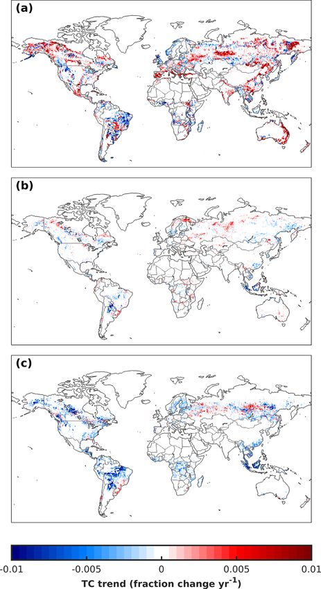
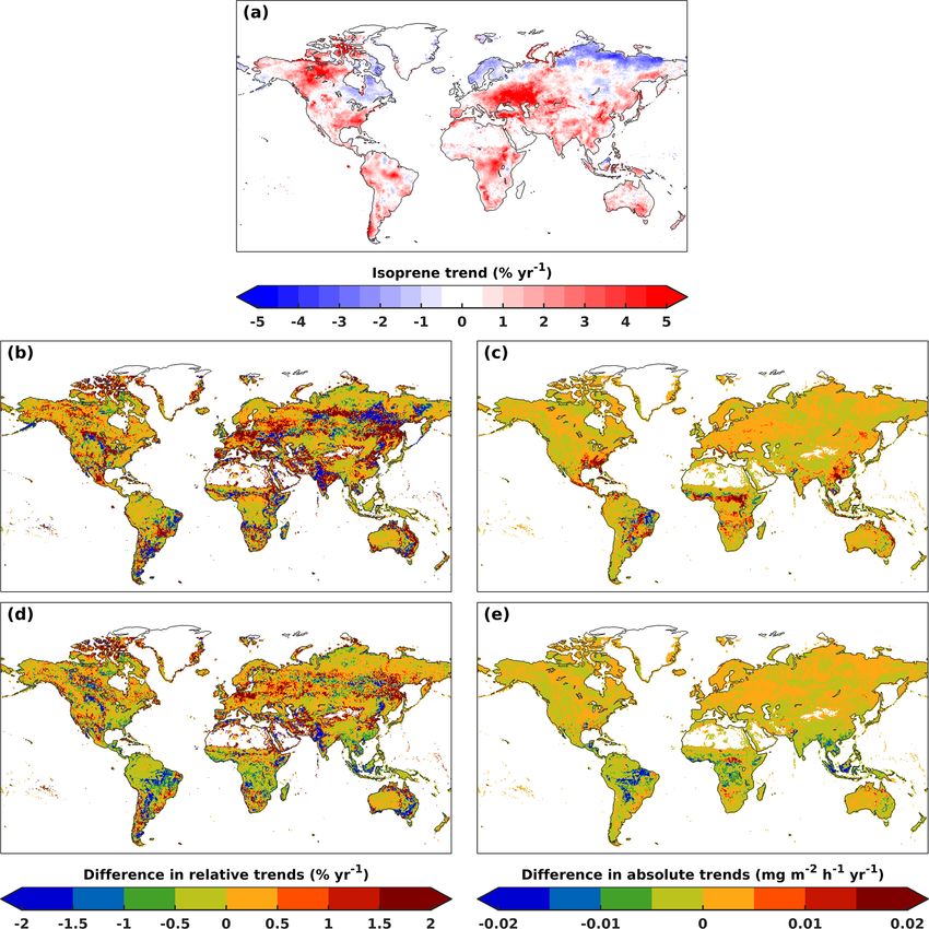
https://doi.org/10.5194/acp-21-8413-2021 Atmos. Chem. Phys., 21, 8413–8436, 20218424 B. Opacka et al.: Impacts of land cover changes on isoprene emissions Figure 5. Distribution of isoprene emissions (in mg m−2 d−1 ) for (a) June–July–August (JJA) and (b) December–January–February (DJF) in 2001 in simulation CTRL, and emission differences of ISOPMOD-CTRL in (c) JJA and (d) DJF and of ISOPGFW-CTRL in (e) JJA and (f) DJF. ily temperature and visible radiation fluxes. Accounting for by about 0.5 % yr−1 according to the parameterization of LULC changes with the MODIS and GFWMOD land cover Possell and Hewitt (2011), whereas the soil moisture stress maps results in a cutback of the global isoprene emission has little impact on trends (Table S6 and Sect. S6 in the Sup- trends by 0.04 and 0.33 % yr−1 , respectively. In ISOPMOD, plement). The effect of LAI trends on global emission trends the deceleration in the global trends pertains to a negative is very small: a positive increment of +0.06 % yr−1 was cal- trend of tropical tree cover in MODIS (Fig. 2) which more culated based on an additional sensitivity simulation in which than compensates for the increasing coverage of temperate LAI interannual variability was omitted. and boreal trees given the large share of the tropics (80 %) The interannual variability (IAV) in isoprene emissions is in the global emissions. In ISOPGFW, the significant de- mainly driven by meteorology and is positively correlated cline in tree cover in all climate zones explains the strong with the Oceanic Niño Index (ONI) (Naik et al., 2004; Lath- drop in the global isoprene emission trend, from 0.94 % to ière et al., 2006; Müller et al., 2008; Stavrakou et al., 2014). 0.61 % yr−1 . Note that the CO2 inhibition effect, not consid- Maxima in isoprene emissions correlate with El Niño events ered in those simulations, would further offset global trends (2002/2003, 2004/2005, 2009/2010, and the 2014–2016), Atmos. Chem. Phys., 21, 8413–8436, 2021 https://doi.org/10.5194/acp-21-8413-2021
B. Opacka et al.: Impacts of land cover changes on isoprene emissions                                                      8425

Figure 6. Time series of global annual isoprene emissions from the CTRL, ISOPMOD, and ISOPGFW simulations.

and minima with La Niña episodes in 2007–2009 (NOAA               tion of trends of ISOPGFW and ISOPMOD is similar since
ONI v5, https://origin.cpc.ncep.noaa.gov, last access: 24 Au-     non-tree PFTs in GFWMOD and MODIS are similar. The
gust 2020). This variability is only weakly dependent on the      decreasing trends in grass and especially shrub cover in low-
choice of land cover dataset. Besides the differences between     emission areas of, for instance, central US, southeast Aus-
long-term trends of the emissions from the three simulations,     tralia, and western India are responsible for the significant
the year-to-year relative changes in emissions are very sim-      relative decreases in isoprene emissions in those areas (left
ilar (Fig. 6). The global minimum and maximum occur in            panels in Fig. 7).
all datasets respectively in 2008 and 2015, whereas the max-         Of the largely forested countries shown in Table 6, Brazil
imum IAV, defined as difference between global maximum            and Indonesia have the highest emissions, of the order of 80
and global minimum (in %), amounts to 20 %, 19.5 %, and           and 30 Tg yr−1 , respectively. Emissions from Russia are low
18 % in simulations CTRL, ISOPMOD, and ISOPGFW, re-               mainly because of the unfavourable climatic conditions and
spectively (Table 5). The impact of interannual variability in    prevalence of low-emitting PFTs (Table S1). China and the
LAI on the variability in isoprene emissions is considered to     US show large discrepancies between estimates using differ-
be either minor (Müller et al., 2008; Stavrakou et al., 2014)     ent LULC databases; e.g. emissions from China vary from
or uncertain because of the large disparities in the long-term    9.5 Tg in ISOPGFW to 23 Tg with ISOPMOD, in the range
evolution of LAI products (Jiang et al., 2017).                   of reported values from previous studies (Stavrakou et al.,
   The isoprene emission trends of the CTRL run illus-            2014; Li et al., 2013). The national emission estimates for
trated in Fig. 7 reflect the temperature and solar radiation      China and Indonesia were significantly lower in the study of
trends (Figs. S4 and S5 in the Supplement). The ability           Stavrakou et al. (2014) also using MEGAN-MOHYCAN, 7
of MEGAN-MOHYCAN to reproduce the response of bio-                and 8 Tg yr−1 over 2005–2012. This difference is largely due
genic emissions to short-term climate variability over veg-       to reduced basal emission rates adopted in that study for trop-
etated areas was demonstrated in Stavrakou et al. (2018)          ical forests over Asia (Stavrakou et al., 2014), based on flux
using spaceborne formaldehyde observations. The simula-           measurements in the rainforest of Borneo (Langford et al.,
tions ISOPMOD and ISOPGFW account for the impact of               2010).
both climate variability and LULC changes. The effect of             Meteorology induces positive trends in all countries, of
LULC changes on emission trends can be estimated from             the order of 0.5 % yr−1 –1.5 % yr−1 in the CTRL run (Ta-
the differences in trends between those simulations and the       ble 6), and is the main driver of the overall trends, except
CTRL run. The differences, namely ISOPMOD-CTRL and                in Russia for which the positive trend induced by LULC
ISOPGFW-CTRL, are shown in the middle and bottom pan-             changes according to MODIS (0.76 % yr−1 ) and exceeds the
els of Fig. 7, respectively. In isoprene-rich areas, the trend    meteorological effect (0.57 % yr−1 ). LULC changes lead to
pattern of ISOPMOD-CTRL and ISOPGFW-CTRL largely                  a reduction in the trends in the US, Brazil, and Indonesia.
reflect trends in tree coverage (Fig. 3). This is because high-   This reduction is most significant for ISOPGFW over Brazil
emitting broadleaf trees are generally dominant in those ar-      (−0.53 % yr−1 ) and Indonesia (−0.7 % yr−1 ). The emission
eas. In less forested regions (low TC), the spatial distribu-     trends over southern China are of opposite sign in ISOPMOD

https://doi.org/10.5194/acp-21-8413-2021                                           Atmos. Chem. Phys., 21, 8413–8436, 2021
You can also read