The 2019 Raikoke volcanic eruption - Part 1: Dispersion model simulations and satellite retrievals of volcanic sulfur dioxide - Recent
←
→
Page content transcription
If your browser does not render page correctly, please read the page content below
Atmos. Chem. Phys., 21, 10851–10879, 2021
https://doi.org/10.5194/acp-21-10851-2021
© Author(s) 2021. This work is distributed under
the Creative Commons Attribution 4.0 License.

The 2019 Raikoke volcanic eruption – Part 1: Dispersion model
simulations and satellite retrievals of volcanic sulfur dioxide
Johannes de Leeuw1 , Anja Schmidt1,2 , Claire S. Witham3 , Nicolas Theys4 , Isabelle A. Taylor5 , Roy G. Grainger5 ,
Richard J. Pope6,7 , Jim Haywood3,8 , Martin Osborne3,8 , and Nina I. Kristiansen3
1 Department  of Chemistry, University of Cambridge, Cambridge, UK
2 Department  of Geography, University of Cambridge, Cambridge, UK
3 Met Office, Exeter, UK
4 Royal Belgian Institute for Space Aeronomy (BIRA-IASB), Brussels, Belgium
5 COMET, Sub-Department of Atmospheric, Oceanic and Planetary Physics, University of Oxford, Oxford, UK
6 School of Earth and Environment, University of Leeds, Leeds, UK
7 National Centre for Earth Observation, University of Leeds, Leeds, UK
8 College of Engineering, Mathematics, and Physical Sciences, University of Exeter, Exeter, UK

Correspondence: Johannes de Leeuw (jd876@cam.ac.uk)

Received: 25 August 2020 – Discussion started: 7 October 2020
Revised: 12 April 2021 – Accepted: 27 April 2021 – Published: 19 July 2021

Abstract. Volcanic eruptions can cause significant disruption   for 12–17 d after the eruption where VCDs of SO2 (in Dob-
to society, and numerical models are crucial for forecasting    son units, DU) are above 1 DU. For SO2 VCDs above 20 DU,
the dispersion of erupted material. Here we assess the skill    which are predominantly observed as small-scale features
and limitations of the Met Office’s Numerical Atmospheric-      within the SO2 cloud, the model shows skill on the order of
dispersion Modelling Environment (NAME) in simulating           2–4 d only. The lower skill for these high-SO2 -VCD regions
the dispersion of the sulfur dioxide (SO2 ) cloud from the      is partly explained by the model-simulated SO2 cloud in
21–22 June 2019 eruption of the Raikoke volcano (48.3◦ N,       NAME being too diffuse compared to TROPOMI retrievals.
153.2◦ E). The eruption emitted around 1.5 ± 0.2 Tg of SO2 ,    Reducing the standard horizontal diffusion parameters used
which represents the largest volcanic emission of SO2 into      in NAME by a factor of 4 results in a slightly increased model
the stratosphere since the 2011 Nabro eruption. We simulate     skill during the first 5 d of the simulation, but on longer
the temporal evolution of the volcanic SO2 cloud across the     timescales the simulated SO2 cloud remains too diffuse when
Northern Hemisphere (NH) and compare our model simula-          compared to TROPOMI measurements.
tions to high-resolution SO2 measurements from the TRO-            The skill of NAME to simulate high SO2 VCDs and the
POspheric Monitoring Instrument (TROPOMI) and the In-           temporal evolution of the NH-mean SO2 mass burden is
frared Atmospheric Sounding Interferometer (IASI) satellite     dominated by the fraction of SO2 mass emitted into the
SO2 products.                                                   lower stratosphere, which is uncertain for the 2019 Raikoke
   We show that NAME accurately simulates the observed          eruption. When emitting 0.9–1.1 Tg of SO2 into the lower
location and horizontal extent of the SO2 cloud during          stratosphere (11–18 km) and 0.4–0.7 Tg into the upper tro-
the first 2–3 weeks after the eruption but is unable, in        posphere (8–11 km), the NAME simulations show a similar
its standard configuration, to capture the extent and pre-      peak in SO2 mass burden to that derived from TROPOMI
cise location of the highest magnitude vertical column den-     (1.4–1.6 Tg of SO2 ) with an average SO2 e-folding time of
sity (VCD) regions within the observed volcanic cloud. Us-      14–15 d in the NH.
ing the structure–amplitude–location (SAL) score and the           Our work illustrates how the synergy between high-
fractional skill score (FSS) as metrics for model skill, NAME   resolution satellite retrievals and dispersion models can iden-
shows skill in simulating the horizontal extent of the cloud    tify potential limitations of dispersion models like NAME,

Published by Copernicus Publications on behalf of the European Geosciences Union.
10852         J. de Leeuw et al.: SO2 dispersion model simulations and satellite retrievals for the 2019 Raikoke eruption

which will ultimately help to improve dispersion modelling
efforts of volcanic SO2 clouds.

1   Introduction

Volcanic activity can vary strongly in intensity, ranging from
passive degassing volcanoes emitting sulfur into the lower
troposphere to explosive eruptions that can release large
amounts of ash and gases high into the stratosphere (e.g.
Oppenheimer et al., 2011). It is well established that vol-
canic eruptions can impact Earth’s climate system through
changes in the energy balance (e.g. Robock, 2000; Schmidt
et al., 2012, 2018; Stenchikov, 2016), which can affect the
hydrological cycle (e.g. Trenberth and Dai, 2007) and atmo-
spheric dynamics (e.g. Shindell et al., 2004). Furthermore,
volcanic air pollution events can lead to a severe and spatially
widespread health hazard and increase excess mortality (e.g.
Schmidt et al., 2011).
   For the aviation industry, ash and gas emissions from             Figure 1. Example of daily TROPOMI overpasses (north of 25◦ N,
volcanic eruptions can pose a flight safety hazard. Flying           with a swath width of 2600 km). Time indicates the approximate
through volcanic ash is a well-recognised hazard as it can           central time for each overpass (each track takes approximately 1.5–
reduce visibility, damage the exterior of the aircraft and com-      2 h). Note the overlap of the swaths, resulting in a higher temporal
promise the functionality of aircraft engines. Ingestion of          resolution near the pole. Also shown is the location of the Raikoke
volcanic ash can cause engine failure and permanently dam-           volcano (triangle) and the radiosonde location at the Petropavlovsk-
age jet engines (Casadevall et al., 1996; Prata and Tupper,          Kamchatsky Airport (square).
2009; Prata et al., 2019; Dunn, 2012). When sulfur diox-
ide (SO2 ) oxidises to sulfuric acid and upon hydration forms
sulfuric acid aerosol particles (see e.g. Hamill et al., 1977;       ern Hemisphere (NH) within the first few weeks after the
Hofmann and Rosen, 1983), damage to the exterior of air-             eruption and was observed by various ground-based observa-
craft can occur (e.g. window crazing) (Bernard and Rose,             tional networks (e.g. Vaughan et al., 2020; Mateshvili et al.,
1990). Through sulfidation, SO2 can also cause serious dam-          2020), aircraft-based instruments (e.g. Bundke et al., 2020)
age to the interior of the engines. Sulfuric acid aerosol par-       and satellites (e.g. Muser et al., 2020; Hyman and Pavolonis,
ticles have been recorded to corrode nickel alloys in engine         2020; Prata et al., 2021; Kloss et al., 2021; Gorkavyi et al.,
components (e.g. compressor blades) when alkali metal salts,         2021) in the following months.
like mineral dust or sea salt, are co-present (Eliaz et al., 2002;      The International Airways Volcano Watch (IAVW) is re-
Grégoire et al., 2018). While this effect has not been linked        sponsible for the dissemination of information on the oc-
to immediate engine failures, it is a concern for the aviation       currence of volcanic eruptions and associated volcanic ash
industry as it increases maintenance costs. Apart from mate-         clouds (ICAO, 2019a) through nine Volcanic Ash Advisory
rial damage, sulfurous odours can also cause distress of cabin       Centres (VAACs). During a volcanic eruption the responsible
passengers and aircrew.                                              VAAC disseminates relevant information to the aviation sec-
   The Raikoke volcano is located in the Kuril Island                tor regarding the geographic location of volcanic ash present
chain, near the Kamchatka Peninsula in Russia (48.3◦ N,              in the atmosphere. Currently, the VAACs are only required
153.2◦ E; see Fig. 1), and had been dormant since 1924.              to provide forecasts of volcanic ash dispersion, and there-
On 21 June 2019 at 18:05 UTC Raikoke started erupting,               fore less development has been achieved on the forecasting
and multiple explosions were reported until 05:40 UTC on             of volcanic gas clouds. There is, however, increasing con-
22 June 2019 (Crafford and Venzke, 2019; Hedelt et al.,              sensus among the scientific community that monitoring and
2019). During this period, Raikoke released the largest              simulating SO2 clouds could be of interest to stakeholders, as
amount of SO2 into the stratosphere since the Nabro erup-            volcanic SO2 can pose a public health hazard and potentially
tion in 2011 (Goitom et al., 2015). The volcanic cloud (while        affect the aviation industry (e.g. increase of aircraft mainte-
a geographic distribution of SO2 and/or sulfate aerosol is not       nance costs) (Witham et al., 2012; Schmidt et al., 2014; Car-
technically a cloud in the meteorological sense, we use this         boni et al., 2016; Granieri et al., 2017; Grégoire et al., 2018).
term through our paper as it is common practice in the atmo-         Volcanic SO2 clouds are also frequently (but not always) co-
spheric dispersion community) dispersed across the North-            located with ash clouds. Detecting ash clouds from satellites

Atmos. Chem. Phys., 21, 10851–10879, 2021                                             https://doi.org/10.5194/acp-21-10851-2021
J. de Leeuw et al.: SO2 dispersion model simulations and satellite retrievals for the 2019 Raikoke eruption                 10853

retrievals remains a challenging task, and in some circum-         The 2019 Raikoke eruption is the first eruption with SO2
stances SO2 clouds may act as proxies for ash clouds (e.g.         emissions in excess of 1 Tg of SO2 that has been observed
Carn et al., 2009; Thomas and Prata, 2011; Sears et al., 2013;     by the TROPOMI instrument. Due to the amount of SO2
Kristiansen et al., 2015). As a result, the latest roadmap pub-    emitted into the stratosphere, it provides an ideal test case to
lished by the IAVW (ICAO, 2019b) includes SO2 forecasts            validate the skill of the Numerical Atmospheric-dispersion
as a core item to be implemented in the future.                    Modelling Environment (NAME) (Jones et al., 2007), which
   The main tools used by VAACs to provide accurate fore-          is the dispersion model used by the London VAAC (Witham
casts of volcanic cloud characteristics are atmospheric dis-       et al., 2020). In this paper we will focus on the evolution
persion models (ADMs), which are numerical models that             of the volcanic SO2 cloud during the first 3 weeks after the
simulate how air parcels disperse within the atmosphere.           2019 Raikoke eruption and compare the output from NAME
ADMs are used for a large variety of advection-related re-         with the TROPOMI and the Infrared Atmospheric Sounding
search, including dust transport, nuclear accidents, forest        Interferometer (IASI) satellite SO2 products. In the accompa-
fires, air pollution, plant diseases and volcanic clouds (Car-     nying Part 2 paper (Osborne et al., 2021), a detailed assess-
penter et al., 2010; Webster et al., 2011; Katata et al., 2015;    ment of the sulfate aerosol together with volcanic ash from
Schmidt et al., 2014, 2015; Ashfold et al., 2017; Meyer et al.,    this eruption is discussed as well as the effects from biomass
2017; Osborne et al., 2019). Because of the ash-focused task       burning aerosols that were emitted into the stratosphere from
of VAACs, there has been a strong research focus on im-            an unusually strong pyrocumulus event in continental North
proving the simulation of volcanic ash in ADMs and mea-            America.
suring volcanic ash using in situ and satellite measurement           The paper is structured as follows: after discussing the
techniques (e.g. Witham et al., 2007; Corradini et al., 2011;      TROPOMI and the IASI satellite SO2 products in Sect. 2.1
Prata and Prata, 2012; Mulena et al., 2016; Harvey et al.,         and 2.2, we briefly introduce all the relevant aspects of the
2018; Webster et al., 2020). The skill of ADMs in simulating       NAME dispersion model in Sect. 2.3, including the erup-
the evolution of SO2 clouds has also been investigated (e.g.       tion source parameters. Using the introduced input param-
Eckhardt et al., 2008; Heard et al., 2012; Boichu et al., 2013;    eters for our 25 d long NAME simulations, we obtain a good
Schmidt et al., 2015) but to a much lesser extent as this has      qualitative comparison of the simulated SO2 cloud with the
generally been the realm of global climate models interested       TROPOMI satellite SO2 products during the first 3 weeks
in the climatic impacts of the periodic stratospheric injections   after the eruption, which we present in Sect. 3.1. A more de-
from volcanoes (e.g. Haywood et al., 2010; Solomon et al.,         tailed analysis of the model skill is presented in Sect. 3.2
2011; Schmidt et al., 2018).                                       and 3.3, where we show that the fractional skill score (FSS)
   Observations are vital in determining the skill of the dis-     and the structure, amplitude and location (SAL) metric (both
persion models. While in situ observations are available           metrics are introduced in Sect. 2.4) are powerful tools for as-
for several well-studied volcanoes (e.g. Pfeffer et al., 2018;     sessing the skill of the model simulations in comparison to
Sahyoun et al., 2019; Whitty et al., 2020), they are only avail-   satellite measurements. The NAME simulation skill in terms
able for a limited number of locations. In recent decades,         of the NH-mean SO2 mass burden throughout the first 25 d
many high-resolution remote-sensing measurements have              after the Raikoke eruption is presented in Sect. 3.4, showing
become available, providing a great data source on activity        a large dependence of the mass burden evolution on the verti-
at even the most remote volcanoes across the globe. A large        cal emission profile. We finish with a discussion of our work
number of satellites now measure atmospheric SO2 , with            (Sect. 4) and present the main conclusions in Sect. 5.
each newly launched instrument having an increased accu-
racy (see for example Fig. 2 in Theys et al., 2019). The TRO-
POspheric Monitoring Instrument (TROPOMI) has been op-             2     Data and methods
erational since the end of 2017 and retrieves atmospheric
SO2 total column densities at an unprecedented spatial reso-       2.1    TROPOspheric monitoring instrument
lution for UV measurements (up to 3.5 km × 5.5 km at nadir)
(Theys et al., 2017, 2019). TROPOMI therefore provides a           TROPOMI is part of the ESA’s S5P satellite launched
useful source of information to evaluate model simulations         on 13 October 2017 (Veefkind et al., 2012) and is a
of SO2 clouds using ADMs (and climate models).                     polar-orbiting, sun-synchronous, hyperspectral spectrome-
   One major issue for the development of ADMs for                 ter that measures Earth-reflected radiances in the ultravio-
volcanic clouds is the relatively small number of large-           let (UV), visible, near-infrared and shortwave infrared parts
magnitude eruptions available since the start of the satel-        of the spectrum. Atmospheric SO2 vertical column den-
lite era in 1979 in order to validate model output. While          sity (VCD, expressed in Dobson units with 1 DU = 2.69 ×
small-magnitude eruptions take place more frequently, large-       1016 molec cm−2 ) is retrieved by applying differential optical
magnitude eruptions that can emit large amounts of SO2 into        absorption spectroscopy (DOAS) (Platt and Stutz, 2008) to
the stratosphere are much more sporadic (e.g. Pyle, 1995;          the measured ultraviolet spectra in three wavelength ranges
Miles et al., 2004; Carn et al., 2016; Schmidt et al., 2018).      (312–326, 325–335 and 360–390 nm). For a more detailed

https://doi.org/10.5194/acp-21-10851-2021                                        Atmos. Chem. Phys., 21, 10851–10879, 2021

10854         J. de Leeuw et al.: SO2 dispersion model simulations and satellite retrievals for the 2019 Raikoke eruption

description of the SO2 retrieval, we refer the reader to Theys
et al. (2017, 2018).
   In our study we use the TROPOMI satellite retrievals
across the NH (north of 25◦ N) that cover the Raikoke
SO2 cloud between 22 June and 15 July 2019. Figure 1
shows an example of the TROPOMI daily overpasses over
the NH. Compared to its predecessors OMI and SCIA-
MACHY, TROPOMI has a higher horizontal pixel resolu-
tion (up to 3.5 km × 5.5 km), allowing for a more detailed
characterisation of the small-scale features in volcanic SO2
clouds (Theys et al., 2019). The retrieved TROPOMI SO2
VCD product is calculated by accounting for a large number
of parameters, such as meteorological cloud fraction, sur-
face albedo and the vertical distribution of absorbing trace
gases (e.g. ozone) (Theys et al., 2017, 2018). As a result,         Figure 2. Estimated total emitted SO2 mass for the Raikoke
                                                                    eruption between 21 June 2019 18:00 UTC and 22 June 2019
the SO2 retrievals from TROPOMI are sensitive to many as-
                                                                    03:00 UTC. The initial emission profile was provided by the Vol-
sumptions, which can lead to uncertainties of up to ±50 %.
                                                                    Res (Volcano Response) team, which is implemented in NAME
For SO2 in the stratosphere, the sum of the various uncertain-      for the 1.5 Tg SO2 simulation (VolRes1.5, orange). We also sim-
ties can be approximated to be around ±30 % of the retrieved        ulated the same profile for a 2.0 Tg SO2 emission (VolRes2.0,
SO2 VCDs. For a detailed discussion of the retrieval uncer-         red). Also included is a new emission profile estimate (StratPro-
tainties, see Theys et al. (2017).                                  file, brown) based on the TROPOMI SO2 VCD cloud on 23 June
   One of the largest uncertainties of the TROPOMI SO2              (see Sect. 2.3.4). This profile has a similar total mass emitted to
VCD product is the height of the SO2 cloud. However, the            VolRes1.5, but a larger fraction (69% instead of 43%) of its mass
sensitivity of the measurement with height is well char-            is emitted in the stratosphere (see Table 2). The grey line rep-
acterised. To account for this sensitivity, the TROPOMI             resents the average tropopause height in the MetUM during the
SO2 VCD level 2 products are publicly available from                first 36 h after the eruption at the location of the Raikoke volcano.
                                                                    The blue line and shading represents the average and the range of
the ESA website (https://s5phub.copernicus.eu, last access:
                                                                    measured tropopause heights by the radiosondes released from the
22 March 2021) for three different scenarios where the SO2
                                                                    Petropavlovsk-Kamchatsky Airport (square in Fig. 1) during the
layer is assumed to be at either 1, 7 or 15 km a.s.l. (above        first 36 h after the eruption.
sea level). The TROPOMI VCD data presented in this study
are for an SO2 layer at 15 km a.s.l., as this is the height near-
est to the estimated weight-averaged emission height for the
Raikoke eruption (see e.g. Fig. 2).                                 age 9 TROPOMI pixels per output grid cell for the reso-
   In order to compare the available satellite retrievals with      lution used in the dispersion model), we have downscaled
any atmospheric dispersion model output, one needs to ap-           the final TROPOMI retrievals to the output grid resolution of
ply the column averaging kernel (AK) operators to the model         the NAME dispersion model by averaging the SO2 VCDs of
data, thereby matching the model-simulated SO2 VCDs to              all pixels within each NAME grid cell (0.2◦ latitude × 0.4◦
the TROPOMI products. The pre-calculated AKs for the                longitude). Unless otherwise specified, we refer to the sulfur
15 km scenario (Theys et al., 2018) have been applied to the        dioxide mass burden as the total SO2 mass within the NH,
NAME model output. We have repeated the analysis using              north of 25◦ N.
the AKs and TROPOMI VCDs assuming the SO2 layer at                     During the initial stage of the eruption, it is likely that
7 km a.s.l., which affects the absolute SO2 VCDs (not shown)        TROPOMI underestimates the SO2 VCDs due to the pres-
but not our interpretation of the results or our overall conclu-    ence of volcanic ash (e.g. Yang et al., 2010). To understand
sions.                                                              if ash interference is likely to have affected our SO2 esti-
   To obtain a daily SO2 mass estimate from the TROPOMI             mates, we also retrieve the absorbing aerosol index (AAI)
measurements, we grid the satellite data and combine all            from the TROPOMI instrument (Zweers, 2016). Although
the overpasses during a 24 h period starting at 12:00 UTC           the TROPOMI AAI product should be used with care due to
of any given day. In the case of multiple overpasses over a         its sensitivity to for example cloud height and optical thick-
single location, we average the SO2 cloud at these grid loca-       ness (see e.g. de Graaf et al., 2016; Kooreman et al., 2020),
tions to avoid double counting. For the mass estimate from          high index values (> 1) indicate the presence of aerosol
TROPOMI we have used a detection threshold of 0.3 DU                plumes from dust outbreaks, volcanic ash and biomass burn-
(Theys et al., 2020). The resulting SO2 VCD (in DU) is then         ing. During the first 48 h after the eruption we found high
converted into a mass (Tg) by using the area of each indi-          peak AAI values within the volcanic cloud (> 18.9 on the
vidual grid point and the molar mass of SO2 . Due to the            22 June and > 3.5 on the 23 June), indicating that volcanic
high spatial resolution of the TROPOMI retrieval (on aver-          ash had an impact on the SO2 retrieval during this period.

Atmos. Chem. Phys., 21, 10851–10879, 2021                                            https://doi.org/10.5194/acp-21-10851-2021
J. de Leeuw et al.: SO2 dispersion model simulations and satellite retrievals for the 2019 Raikoke eruption                10855

2.2   The infrared atmospheric sounding interferometer            2.3.1   Simulating volcanic cloud dispersion using
                                                                          NAME
The second satellite SO2 dataset used in our analysis is ac-
quired using IASI aboard the MetOp-A and MetOp-B satel-           Simulating the dispersion of a volcanic cloud with NAME
lites. These satellites operate in tandem on a polar orbit with   relies on the tracing of air parcels through the atmosphere,
a field of view (FOV) consisting of four circular footprints of   each containing an ash, SO2 and/or SO4 mass. These air
12 km diameter (at nadir) inside a square of 50 km × 50 km        parcels are released from the source location (volcano),
and provide a global coverage twice a day. For our analysis       where the user has to define the eruption source param-
we use the SO2 plume height estimates based on the IASI           eters (see Sect. 2.3.4). NAME is an offline model; there-
data, which are produced by applying the retrieval algorithm      fore, each parcel is advected by an externally obtained
presented in Carboni et al. (2012, 2016). The IASI instru-        wind field (e.g. a high-resolution Numerical Weather Pre-
ment also retrieves the SO2 VCDs within the volcanic plume        diction (NWP) model). In our simulations, we use the wind
but uses a different set of assumptions in the retrieval algo-    fields from the latest global analysis of the Met Office Uni-
rithm compared to TROPOMI (e.g. IASI retrieves the plume          fied Model (MetUM), which have a horizontal resolution of
height which affects the SO2 VCD; the retrieved IASI plume        around 10 km at mid-latitudes, 59 levels between the surface
height can be different from the plume heights assumed in         and 30 km a.s.l. (decreasing vertical resolution with altitude,
the TROPOMI product, and therefore the SO2 VCDs from              with approximately 600 m resolution at tropopause height),
the two methods are not equivalent). To compare SO2 VCDs          and a 3-hourly temporal resolution. The path of each trajec-
from NAME to the IASI data, one would therefore also need         tory is calculated using the following equation:
to apply a different scaling (i.e. AK). As the TROPOMI
                                                                  x(t + 1t) = x(t) + [u(x(t)) + u0 (x(t))]1t,                 (1)
and IASI retrieval assumptions and limitations are satellite-
specific (for example, TROPOMI might detect SO2 closer to         where x(t) is the location of the parcel at time t, x(t + 1t)
the surface than IASI due to the presence of water vapour),       is the new location of the parcel at time t + 1t, u(x(t)) is
a comparison between the two SO2 VCD products is not              the 3D-wind vector at location x(t) and u0 (x(t)) represents
straightforward and is not attempted here. While it would         a stochastic perturbation to the parcel trajectory represent-
be an interesting exercise to apply our analysis also to the      ing turbulence and unresolved sub-grid mesoscale wind vari-
IASI data, we focus on the comparison of NAME with the            ations in the dispersion model. In NAME, u0 consists of two
TROPOMI SO2 estimates, and therefore no further analysis          parts representing atmospheric turbulence (u0turb ) and sub-
is done for the IASI SO2 VCD retrievals.                          grid mesoscale diffusion (u0meso ). The turbulence part repre-
                                                                  sents the stochastic motions from the air parcels due to small-
2.3   Numerical Atmospheric-dispersion Modelling                  scale perturbations. The mesoscale diffusion represents the
      Environment (NAME)                                          horizontal mesoscale motions in the atmosphere that are not
                                                                  captured by the resolution of the used NWP model. Each
The Numerical Atmospheric-dispersion Modelling Environ-           NWP model has a limited spatial and temporal resolution,
ment (NAME) is a Lagrangian model developed by the Met            and as a result part of the mesoscale features (e.g. eddies) are
Office (Jones et al., 2007) and is the operational dispersion     not captured by the NWP wind field provided. Both the tur-
model used by the London VAAC to forecast the dispersion          bulence and mesoscale diffusion within the free atmosphere
of volcanic clouds within European airspace (e.g. the Ice-        (excluding the planetary boundary layer, which has a more
landic eruptions of Eyjafjallajökull in 2010 and Holuhraun        detailed scheme; Webster et al., 2018) are calculated using
in 2014–2015). For our work we use NAME version 8.1. The                         p
model can trace both ash particles and gases through the at-      u0turb · 1t = d 2K turb · 1t,                                (2)
mosphere and includes chemistry parameterisations that al-
                                                                                  p
                                                                  u0meso · 1t = d 2K meso · 1t,                                (3)
low the conversion of SO2 into sulfate aerosols (SO4 ) within
                                                                              2    2      2
the volcanic cloud (see Sect. 2.3.3). There is no radiative or    K x = σu τu , σv τv , σw τw ,                                (4)
chemical interaction between the ash particles and the sulfur
                                                                  where K x is a 3D-diffusion vector defined separately for both
species in NAME; the ash particles and sulfate aerosols are
                                                                  components, using typical values for the standard deviation
thus considered to be externally mixed. In this section we fo-
                                                                  of the velocity (σ ) and typical time length scales (τ ). d rep-
cus on the dispersion of SO2 and highlight the important as-
                                                                  resents a random number from a top-hat distribution within
pects of NAME for this part of the research. More details on
                                                                  the range [−1, 1]. The values for σ and τ are dependent on
the modelling of ash particles within the model are discussed
                                                                  the NWP model used, as they are impacted by the resolution
in the accompanying Part 2 paper (Osborne et al., 2021).
                                                                  of the model (Harvey et al., 2018; Webster et al., 2018). The
                                                                  values for σ and τ used in this study are obtained from the
                                                                  analysis done by Webster et al. (2018) and are shown in Ta-
                                                                  ble 1. Note that for K meso the vertical component (σw2 τw ) is
                                                                  zero.

https://doi.org/10.5194/acp-21-10851-2021                                       Atmos. Chem. Phys., 21, 10851–10879, 2021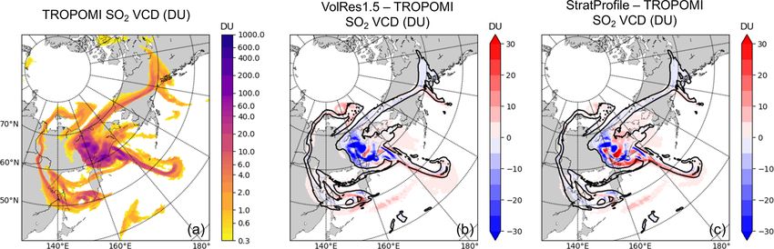
10856            J. de Leeuw et al.: SO2 dispersion model simulations and satellite retrievals for the 2019 Raikoke eruption

Table 1. The values for the diffusion parameter K used in NAME.          Table 2. Overview of the NAME simulations performed using dif-
Values are NWP dependent and are given here for the Met Office           ferent emission profiles and a reduced mesoscale diffusion (values
Unified Model global analysis (10 km horizontal resolution, 59 lev-      for Kmeso can be found in Table 1). Also shown is the estimated
els) with a 3-hourly temporal resolution. Values for σ 2 are given       mass emitted into the stratosphere. For the actual vertical emission
instead of σ to be consistent with the values presented by Webster       profiles, see Fig. 2. All the simulations use the same NWP data input
et al. (2018). Values are given for both the turbulence K turb and       (Global MetUM), the same emission location (48.3◦ N, 153.2◦ E),
the mesoscale diffusion K meso that are used in NAME for the free        and duration between 21 June 2019 18:00 UTC–22 June 2019
atmosphere (i.e. excluding the boundary layer).                          03:00 UTC. The simulation domain is the NH between 25–90◦ N
                                                                         and the simulation length is 25 d.
        Global MetUM analysis (0.140625◦ × 0.09375◦ , 59 levels,
                        3-hourly resolution)                              Simulation         Mass    Profile            Mass       Mesoscale
                                                                          name             emitted   used           stratosphere   diffusion
                 K (m2 s−1 )           2
                                     σu,v      τu,v        σw2     τw
                                 (m2 s−2 )      (s)   (m2 s−2 )    (s)    VolRes1.5         1.5 Tg   VolRes1.5        0.64 Tg      Kmeso
                                                                          VolRes2.0         2.0 Tg   VolRes2.0        0.85 Tg      Kmeso
 K turb      (18.75, 18.75, 1)     0.0625       300       0.01     100    StratProfile     1.57 Tg   StratProfile     1.09 Tg      Kmeso
 K meso       (6400, 6400, 0)        0.64    10 000          0       0    VolRes1.5rd       1.5 Tg   VolRes1.5        0.64 Tg      0.25 Kmeso
                                                                          StratProfilerd   1.57 Tg   StratProfile     1.09 Tg      0.25 Kmeso

   Accurately describing atmospheric dispersion due to mix-
ing is a complex three-dimensional problem (e.g. Waugh                   total mass of the SO2 of all parcels in each grid box every
et al., 1997; Haynes and Anglade, 1997; Haynes and Shuck-                hour. The NAME output is calculated using a grid size of 0.2◦
burgh, 2000; Hegglin et al., 2005; Wang et al., 2020).                   latitude and 0.4◦ longitude (approximately 20 km × 20 km at
TROPOMI satellite retrievals provide SO2 VCDs, and there-                the latitude of the Raikoke volcano). The vertical resolution
fore our information on mixing effects of the SO2 cloud is               of the output is 500 m up to 15 km a.s.l. and 1 km resolution
limited to their horizontal impact. Studies by Balluch and               up to 20 km a.s.l., giving a total of 35 levels.
Haynes (1997) and Haynes and Anglade (1997) have shown                      To compare the daily SO2 mass estimates from NAME and
that the vertical and horizontal components of stratospheric             TROPOMI, we select the hourly NAME output correspond-
mixing are related, which allowed them to derive an effec-               ing to each individual TROPOMI overpass time and select
tive horizontal diffusion from observations. Values reported             only the grid boxes in NAME that are in the domain scanned
in the literature for horizontal diffusion coefficients in the           by TROPOMI during that overpass. To calculate the SO2
lower stratosphere vary over an order of magnitude (103 –                VCD, we apply the corresponding column AK operators ob-
105 m2 s−1 ) and also depend on the resolution of the NWP                tained from TROPOMI (see Sect. 2.1) to each grid cell of the
data used (e.g. Balluch and Haynes, 1997; Waugh et al.,                  NAME output. Then for each column on the NAME output
1997; Harvey et al., 2018; Wang et al., 2020). To investigate            grid, the SO2 concentrations (kg m−3 ) in each grid cell are
the importance of the horizontal mesoscale diffusion param-              vertically integrated to obtain the SO2 VCD estimate from
eter, we present two sensitivity simulations with two differ-            NAME.
ent SO2 emissions profiles (see Sect. 2.3.4 for discussion of               In all our NAME simulations we found that the SO2 cloud
these profiles) and a reduced value for K meso (see Table 2).            is more diffuse than observed by TROPOMI. Therefore, re-
We decided to only change the K meso parameter, as the hor-              moving all SO2 VCDs < 0.3 DU in NAME (which is the de-
izontal K turb components (see Table 1) are at least an order            tection threshold we have used for TROPOMI; see Sect. 2.1)
of magnitude smaller than the K meso components, and thus                from the simulations would result in a negative bias within
changing them would not show any significant impact on our               the NAME simulation mass estimates that are not related to
initial results that is not captured by changing K meso . The            the evolution of the cloud but due to the stronger diffusion
simulations with a reduced value for K meso are indicated by             within the model. Therefore we have not included a detec-
the subscript rd throughout this study. Due to the large range           tion threshold when determining the SO2 mass estimates for
of potential realistic K meso values, we have stepwise reduced           the NAME simulations. Similarly to the TROPOMI estimate,
the parameter and found the best results for a 75 % reduction,           the daily mass estimates from NAME are calculated during a
which is the value presented in this paper and is similar to the         24 h period starting at 12:00 UTC on any given day. The SO2
values reported by Balluch and Haynes (1997) and Waugh                   mass burden is defined as the total SO2 mass (Tg) within
et al. (1997).                                                           the NH, north of 25◦ N.

2.3.2     Calculating SO2 mass estimates from NAME                       2.3.3   Chemistry within NAME

In our simulations, the SO2 concentrations (kg m−3 ) from all            NAME contains an atmospheric chemistry scheme (Reding-
the individual air parcels in NAME are presented as hourly               ton et al., 2009). The relevant chemistry for volcanic clouds
means on a regular latitude–longitude grid by calculating the            is related to the conversion of SO2 into sulfate (SO2−    4 ).

Atmos. Chem. Phys., 21, 10851–10879, 2021                                                  https://doi.org/10.5194/acp-21-10851-2021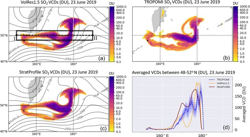
J. de Leeuw et al.: SO2 dispersion model simulations and satellite retrievals for the 2019 Raikoke eruption                10857

NAME accounts for the oxidation of SO2 in the gas phase          (4) vertical emission profile, and for simulating volcanic ash
using the following reaction:                                    also (5) particle density, shape and particle size distribution.
                                                                 Here we will discuss ESP 1–4. For information about the set-
OH + SO2 + M → HSO3 + M,                                 (R1)    up of the simulations including ash, we refer to the Part 2
                                                                 paper (Osborne et al., 2021). For all simulations described
where HSO3 is then rapidly oxidised to H2 SO4 on formation.      in this paper, we released a total of 10 million air parcels in
When water is present in the atmosphere, the oxidation can       NAME within a column above the volcano, with each parcel
happen in the aqueous phase by both H2 O2 and O3 through         representing an equal amount of SO2 mass. All simulations
the following reaction:                                          are run for 25 d until 15 July 2019, and the simulation domain
                                                                 is the NH (north of 25◦ N).
SO2 + H2 O     H+ + HSO−
                       3,                                (R2)       In all our simulations (see Table 2 for overview),
HSO−
   3      H+ + SO2−
                 3 ,                                     (R3)    we release the SO2 from the location of the volcano
                                                                 (48.3◦ N, 153.2◦ E) between 21 June 18:00 UTC and 22 June
which is followed by                                             03:00 UTC. The timing of the SO2 release is in line with
                 2−
                                                                 the source term provided by the Volcano Response (VolRes)
HSO−                  +
   3 + H2 O2 → SO4 + H + H2 O,                           (R4)    team (https://wiki.earthdata.nasa.gov/display/volres, last ac-
                2−
HSO−                +
    3 + O3 → SO4 + H + O2 ,                              (R5)    cess: 6 July 2021). The VolRes team is an international re-
                                                                 search collaboration to coordinate a response plan after large
SO2−           2−
  3 + O3 → SO4 + O2 .                                    (R6)    volcanic eruptions using observational and modelling tools.
                                                                 No information on the temporal variation in the mass erup-
Reactions (R2)–(R6) dominate in cloudy conditions and only
                                                                 tion rate was provided by VolRes; thus we assume a constant
occur in model grid boxes when both the meteorological
                                                                 mass eruption rate throughout the entire eruption period.
cloud fraction and liquid water content are non-zero. The
                                                                    The Raikoke eruption injected most SO2 mass near the
concentrations of H2 O2 and O3 in the atmosphere are pre-
                                                                 tropopause height (see Fig. 2), but the precise emission pro-
defined in the NAME model by using monthly mean back-
                                                                 file is uncertain (e.g. Hedelt et al., 2019; Kloss et al., 2021).
ground fields obtained from a historical Unified Model cou-
                                                                 Small changes in the SO2 emission profile could lead to a
pled to the United Kingdom Chemistry and Aerosol model
                                                                 large change in the amount of mass emitted into the strato-
(UM-UKCA model) simulation that have been smoothed be-
                                                                 sphere, which will strongly influence the evolution of the
tween months using interpolation.
                                                                 SO2 cloud. Therefore, in our study we use three different
   In NAME the SO2 and sulfate aerosol particles can be re-
                                                                 SO2 emission profiles that vary in terms of the SO2 mass
moved through dry and wet deposition. For our simulations
                                                                 that is emitted into the stratosphere as shown in Fig. 2. The
we found that the dry deposition had limited importance for
                                                                 VolRes1.5 SO2 emission profile is based on the vertical mass
the 2019 Raikoke eruption as most of the volcanic clouds are
                                                                 distribution obtained from the VolRes team using IASI re-
at high altitudes. Wet deposition in NAME is calculated us-
                                                                 trievals on 22 June, as shown by the orange bars in Fig. 2.
ing a standard depletion equation:
                                                                 The total SO2 mass emitted based on the VolRes estimate,
dC                                                               which is also the mass emission used in the VolRes1.5 pro-
   = 3C,                                                   (5)   file, was approximately 1.5 ± 0.2 Tg of SO2 .
dt
                                                                    To determine what fraction of the total SO2 mass was emit-
3 = Ar B ,                                                 (6)
                                                                 ted into the stratosphere, we calculated the tropopause height
with C representing the SO2 concentration (kg m−3 ) and 3        in the MetUM global analysis using the World Meteorolog-
the scavenging coefficient, which is calculated based on the     ical Organization (WMO) temperature lapse rate definition.
rainfall rate r (in mm h−1 ) and two scavenging parameters A     Using the spread in the 150 nearest grid points to the vol-
and B. The parameters A and B vary for different types of        cano location in the model, we get an average tropopause
precipitation (i.e. large-scale/convective and rain/snow) and    height of 11.2±0.7 km during the first 36 h after the eruption.
for different wet deposition processes (i.e. rainout, washout    To verify this tropopause height, we used radiosonde data
and the seeder–feeder process). For more detailed informa-       from the Petropavlovsk-Kamchatsky Airport (see Fig. 1),
tion, including the specific values for A and B for SO2 and      which is the nearest radiosonde location to the Raikoke vol-
sulfate aerosols, we refer to Webster and Thomson (2014),        cano (data can be retrieved from http://weather.uwyo.edu/
Leadbetter et al. (2015) and references therein.                 upperair/sounding.html, last access: 6 July 2021). Using the
                                                                 same tropopause height criteria for the radiosondes released
2.3.4   Eruption source parameters                               from this location, we estimate an average tropopause al-
                                                                 titude of 10.5 ± 0.7 km during the first 36 h, showing that
When simulating a volcanic eruption, the NAME dispersion         the MetUM simulated the tropopause height within the ex-
model needs eruption source parameters (ESPs) consisting of      pected range. Using the MetUM tropopause height estimate,
(1) location, (2) timing, (3) mass eruption rate (kg s−1 ) and   the VolRes1.5 profile emits 0.86 Tg into the upper tropo-

https://doi.org/10.5194/acp-21-10851-2021                                      Atmos. Chem. Phys., 21, 10851–10879, 2021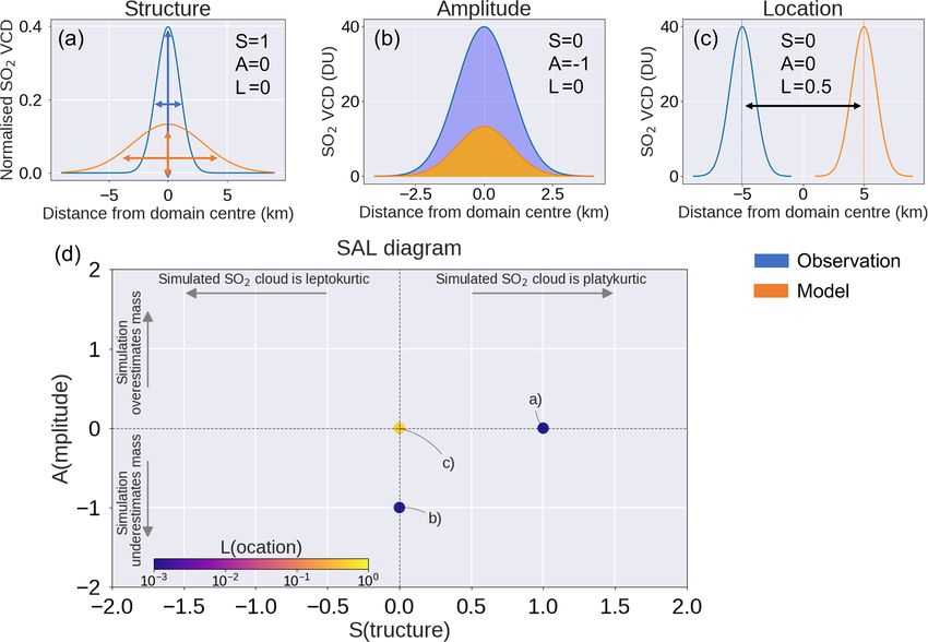
10858         J. de Leeuw et al.: SO2 dispersion model simulations and satellite retrievals for the 2019 Raikoke eruption

sphere (UT) with a peak at 10 km altitude and emits 0.64 Tg         after the eruption. The study by Muser et al. (2020) shows
into the lower stratosphere (LS, defined as the layer between       that after the Raikoke eruption, most of the radiative lofting
the tropopause and 18 km a.s.l.) with a secondary peak at           of the ash layers occurred over these timescales, and we as-
14 km a.s.l.                                                        sume similar timescales to be applicable for the lofting of
   In the case of a multi-phase plume like Raikoke (multi-          the SO2 clouds. Reducing the horizontal diffusion K meso in
phase here refers to the mixture of ash, sulfate aerosols and       the VolRes1.5rd simulation (not shown) resulted in a similar
gas present in the cloud, not the number of eruption phases),       underestimate as shown in Fig. 3d for VolRes1.5, excluding
high ash concentrations within the volcanic cloud can inter-        that overdispersion in the stratosphere is the main source for
fere with satellite SO2 retrievals (Yang et al., 2010; Carboni      the underestimate.
et al., 2016; Theys et al., 2017), leading to an underestima-          Based on the initial findings from the VolRes1.5 simula-
tion of the SO2 VCDs. Furthermore it is known that, in the          tion, we also conduct a simulation in which we released a
stratosphere, ash and sulfate aerosols can have a local heat-       total of 2 Tg of SO2 , using the same relative mass distribu-
ing effect due to their interactions with radiation, resulting      tion in the vertical, termed VolRes2.0. The experiment emits
in lofting of the SO2 , sulfate aerosols and ash (e.g. Niemeier     a larger amount of SO2 into the LS (1.15 Tg in the UT and
et al., 2009; Jones et al., 2016; Muser et al., 2020; Bruckert      0.85 Tg in the LS). In chemistry transport models (including
et al., 2021). NAME does not account for radiative lofting of       NAME), the chemical conversion and the rate of wet and dry
volcanic species due to changes in heating rates as it is an of-    deposition of SO2 depends on the SO2 concentration. There-
fline model driven by NWP wind fields that are not affected         fore this simulation is not a simple scaling of the VolRes1.5
by any volcanic ash or aerosols radiative effects.                  results.
   The fact that Raikoke was an eruption that produced a               In addition, we derive a different vertical profile based on
multi-phase plume that emitted 1.5 Tg of SO2 and 15 Tg of           the TROPOMI SO2 VCD retrievals (StratProfile; for deriva-
ash (Osborne et al., 2021) near the tropopause (see Fig. 2)         tion see Appendix A) in which we use a different relative
justifies simulations using different initial SO2 emission pro-     mass distribution in the vertical. In contrast to the VolRes1.5
files and warrants a closer investigation of the emission pro-      profile (which is based on the IASI satellite overpasses on
file provided by the VolRes team. To understand potential           22 June), our StratProfile emission profile is based on the
uncertainties on the VolRes emission profile, we have run           23 June overpasses of TROPOMI. These overpasses are ap-
an initial 36 h NAME simulation with the VolRes1.5 verti-           proximately 30 h after the onset of the eruption and show
cal emission profile input and compared the SO2 VCD es-             a reduced ash interference (as seen by the strongly reduced
timates (Fig. 3a) with the TROPOMI retrieval on 23 June             AAI values; see Sect. 2.1); thus we expect the SO2 retrievals
(Fig. 3b). The comparison reveals that the VolRes1.5 simula-        to be more accurate. Furthermore, this effective emission
tion has a different longitudinal distribution compared to the      profile (Rix et al., 2009; Klüser et al., 2013) will take into
TROPOMI satellite retrievals. Figure 3d shows the averaged          account any lofting of the SO2 clouds resulting from the ra-
SO2 VCDs between 48–52◦ N along section I–II (black box             diation interactions which may be enhanced by the presence
in Fig. 3a) for the clouds shown in Fig. 3a–c. This shows that      of ash during the first 30 h after the eruption. The derived
along the northern part of the cloud between 170–175◦ E, the        StratProfile emission profile releases similar amounts of SO2
VolRes1.5 simulation underestimates the SO2 VCDs from               into the atmosphere as the VolRes1.5 run (1.57 Tg) but has
TROPOMI by up to a factor of 8.                                     the main peak in SO2 mass at 12–13 km altitude. As a re-
   Figure 4 shows the vertical cross section from the Vol-          sult, the StratProfile emits a much higher fraction (69 % or
Res1.5 simulation through the SO2 cloud along section I–II          1.09 Tg) of the mass into the LS (VolRes emission profile
in Fig. 3a, together with the available estimated cloud heights     emits 43 % or 0.64 Tg into the LS).
from IASI for all pixels between 49–50◦ N. The cloud height
from the IASI retrieval is estimated using the method de-           2.4   Metrics to determine the skill of the NAME
scribed in Carboni et al. (2016). Figure 4 shows that the                 simulations
SO2 cloud between 170–175◦ E is simulated in NAME be-
tween 11–14 km, which coincides with the UT/LS in the               Assessing the model’s skill in representing satellite measure-
MetUM Global model (see Fig. 2). The altitude of the SO2            ments of SO2 requires appropriate metrics. Similar compar-
cloud for the NAME VolRes1.5 simulation along the cross             isons should be possible in almost near-real time for VAACs
section shown in Fig. 4 is within the uncertainty range of          when investigating future eruptions. Therefore, apart from
the IASI height estimates and gives us confidence that the          being able to show the details of the model–satellite compar-
NAME simulated cloud height range is realistic. However,            ison, it is also important that the metric is easily interpretable
the underestimated SO2 VCDs in the latitude range 170–              by end users. In the following subsections we introduce two
175◦ E for the VolRes1.5 simulation compared to TROPOMI             metrics for identifying the skill of the simulations: (1) the
(Fig. 3) could indicate an underestimation of the mass frac-        FSS and (2) the SAL score.
tion of SO2 present in the stratosphere, which could be due
to the lack of radiative lofting of the SO2 during the first 36 h

Atmos. Chem. Phys., 21, 10851–10879, 2021                                            https://doi.org/10.5194/acp-21-10851-2021
J. de Leeuw et al.: SO2 dispersion model simulations and satellite retrievals for the 2019 Raikoke eruption 10859
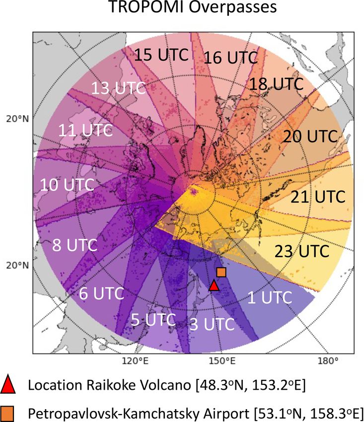
Figure 3. The SO2 VCD estimates for 23 June 2019 for (a) the VolRes1.5 simulation, (b) the TROPOMI retrievals and (c) the StratProfile
simulation. The TROPOMI retrievals are downscaled to the NAME simulation resolution, (i.e. averaged per grid box; see Sect. 2.1). The
black contours show the pressure at the 10 km a.s.l. in the MetUM analysis used for both NAME simulations. Panel (d) shows the latitudinal
SO2 VCDs from panels (a)–(c) along section I–II in panel (a), averaged over the black box between 48 and 52◦ N. Shading represents the
standard error estimate for the TROPOMI estimate.
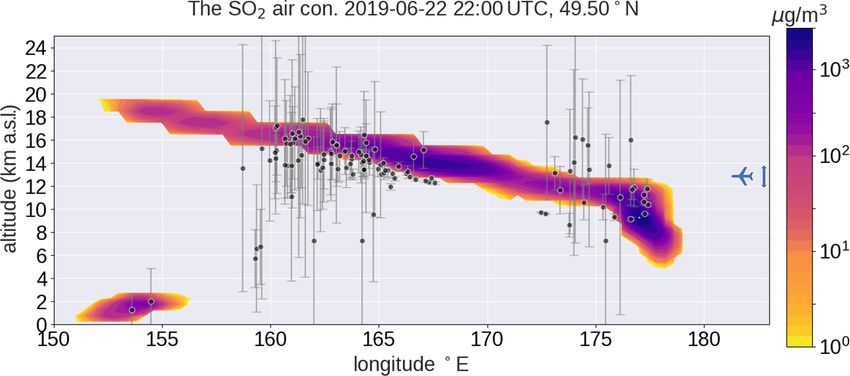
Figure 4. Vertical cross section of SO2 mass concentrations (µg m−3 ) in the VolRes1.5 simulation and the IASI height estimate along the
line I–II in Fig. 3a on 22 June 2019 at 22:00 UTC. This time corresponds with the IASI overpass over the volcanic cloud, thereby minimising
displacement errors due to timing. The black dots represent the available height estimates including error bars from the IASI retrieval of the
SO2 cloud for all pixels between 49–50◦ N, and it is estimated following the method described in Carboni et al. (2016). The blue arrow on
the right of the figure indicates the range of cruise altitudes for long-haul aircraft (11.9–13.7 km).
2.4.1 Fractional skill score (FSS) (Dacre et al., 2016; Harvey and Dacre, 2016). For volcanic
SO2 clouds, the FSS is calculated using the ratio between the
model-simulated (Mk ) and observed (Ok ) fractional cover-
The FSS was originally developed to determine the skill of
age of the SO2 cloud at each location (neighbourhood) in the
weather forecast models to represent radar rainfall observa-
domain investigated. When considering N neighbourhoods,
tions (Roberts, 2008; Roberts and Lean, 2008; Mittermaier
the FSS is calculated using
et al., 2013) but has been since used to also describe the
skill of dispersion models in representing volcanic clouds
https://doi.org/10.5194/acp-21-10851-2021 Atmos. Chem. Phys., 21, 10851–10879, 2021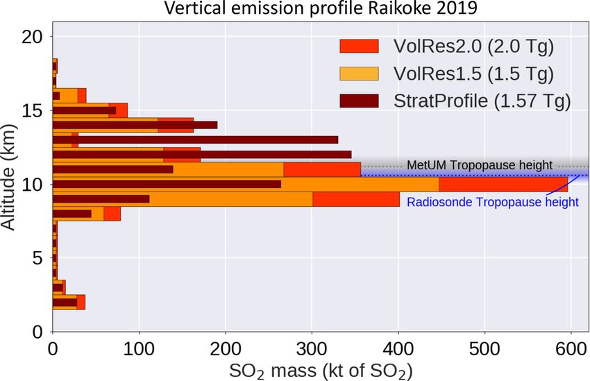
10860        J. de Leeuw et al.: SO2 dispersion model simulations and satellite retrievals for the 2019 Raikoke eruption

                                                                  observed SO2 clouds. In our analysis each cloud is identi-
            FBS                                                   fied as a group of adjacent grid cells which have a SO2 VCD
FSS = 1 −         ,                                        (7)
           FBSref                                                 value above a certain threshold. From Theys et al. (2019) we
        1 XN                                                      deduce that the detection limit of the satellite measurements
FBS =         (Ok − Mk )2 ,                                (8)    for individual pixels is approximately 1 DU. All of the analy-
       N k=1
                                                                  sis in our study is done at the highest resolution that is avail-
                                                                  able for all fields, which is the NAME model output (0.2◦ lat-
            "                  #
               N        N
          1 X       2
                      X
                             2
FBSref =         O −        M .                            (9)    itude and 0.4◦ longitude). Due to the higher spatial resolution
          N k=1 k k=1 k
                                                                  of the satellite product, we have to average the TROPOMI
The FSS is calculated from the fractions Brier score (FBS),       output of multiple pixels within each NAME grid box (on
which is a variation on the Brier score (Brier, 1950), and        average 9 TROPOMI pixels per NAME output grid box at
FBSref is the largest FBS score one can obtain from multi-        each given time step) to get both datasets on the same output
ple non-zero fractions within the domain when there is no         grid. As a result, we have used a lower detection threshold
overlap between the two fields. In the case that observations     of 0.3 DU when identifying all grid points that are part of a
and simulation are perfectly aligned, FSS is equal to one. In     SO2 cloud for the (re-gridded) TROPOMI retrievals and the
the case of a total mismatch FSS is equal to zero. In general     NAME simulations. To remove additional spurious data from
for the FSS, a model simulation is considered to have skill       the TROPOMI satellite product, we also include a minimum
when FSS > 0.5 (see e.g. Harvey and Dacre, 2016).                 size of each identified SO2 cloud to be 100 km2 (approxi-
   The FSS metric is very suitable for studying the skill of a    mately the NAME grid box size at 50◦ N) before consider-
model in capturing the volcanic cloud’s spatial extent. One       ing in our analysis. Simulated and observed SO2 VCD val-
advantage of using the FSS metric is that it relaxes the re-      ues below either of these thresholds are excluded from all S,
quirement for exact matching of the spatial features in the       A and L calculations. SAL scores have been calculated by
simulations with the observations. Instead when the frac-         comparing the SO2 VCD estimates from each NAME simu-
tional coverage of the SO2 cloud within a studied region          lation with the individual TROPOMI overpasses, as well as
(i.e. a neighbourhood of size N) is the same for the obser-       the daily averages. When calculating the individual overpass
vations and the simulation, this metric counts it as a cor-       SAL score values, we only included the NAME simulation
rect forecast. By using different sizes of neighbourhoods, one    data within the region covered by the TROPOMI overpass.
can also determine at which spatial resolution the simula-           To interpret the SAL score, we first assume a single ide-
tion is skilful (i.e. for which N is FSS > 0.5) at any given      alised 2D-Gaussian-shaped cloud for both the simulated and
time, which helps to determine at which spatial scale fea-        observed SO2 VCDs. Looking at the schematic cross section
tures of the SO2 cloud can be considered realistic. However       presented in Fig. 5, three characteristics are represented by
the method does not consider differences in SO2 VCDs val-         the S, A and L scores. The S score compares the shapes of
ues – it only considers a “hit” or “miss” for each location.      each individual SO2 cloud in terms of the horizontal extent
By applying the same FSS metric to increasing SO2 VCD             (width) and maximum concentrations within the cloud, by
thresholds (i.e. subregions of the cloud), one can obtain in-     comparing the normalised shape of the clouds (i.e. total mass
formation about model skill at simulating volcanic SO2 cloud      of the simulated and the observed clouds are made equal; see
structures with varying vertical column densities.                Fig. 5a). A negative S score indicates that the simulated SO2
                                                                  clouds are too narrow or have peak SO2 VCD values that are
2.4.2   Structure, amplitude and location score (SAL              too high when compared to the observed cloud (leptokurtic).
        score)                                                    When the simulated SO2 clouds are too wide spread or have
                                                                  peak SO2 VCD values that are too low, this is indicated by a
The SAL score is a metric that is composed of three com-          positive S score (platykurtic).
ponents, which describe the structure (S), amplitude (A) and         The A score represents the comparison between the sim-
location (L) of an investigated feature within a specified do-    ulated and the observed total mass of SO2 within the entire
main. The metric was originally developed to compare the          studied domain and is independent on the number of individ-
structure of model-simulated precipitation fields with ob-        ual SO2 clouds. Negative A scores represent an underesti-
servations (Wernli et al., 2008) but has since been adapted       mate of the total SO2 mass in the simulation when compared
to also describe other fields, including volcanic clouds (e.g.    to the observations (Fig. 5b), while a positive value shows
Dacre, 2011; Wilkins et al., 2016; Radanovics et al., 2018).      that the simulation is overestimating the total SO2 mass in
Here we will adopt this metric to describe the evolution of the   the domain.
SO2 cloud. For a detailed description of the equations used          Finally the L score represents the distribution of the in-
to calculate each individual component, we refer the reader       dividual simulated and observed SO2 clouds within the do-
to Wilkins et al. (2016).                                         main and consists of two parts: L1 and L2 (Wernli et al.,
   Briefly, to calculate the S and L scores (not needed for the   2008). L1 represents the normalised distance between the
A score), we have to identify all the individual simulated and    domain-averaged centre of mass of all the simulated and ob-

Atmos. Chem. Phys., 21, 10851–10879, 2021                                         https://doi.org/10.5194/acp-21-10851-2021
J. de Leeuw et al.: SO2 dispersion model simulations and satellite retrievals for the 2019 Raikoke eruption 10861 Figure 5. Schematic overview of the SAL score and its interpretation, using two cross sections of idealised Gaussian-shaped SO2 clouds. Each panel shows the impact of an individual component of the SAL score: (a) structure, (b) amplitude and (c) location (only the L1 part). A negative S score indicates that the simulated SO2 clouds are too narrow or have peak SO2 VCD values that are too high when compared to the observed cloud (leptokurtic). When the simulated SO2 clouds are too wide spread or have peak SO2 VCD values that are too low, this is indicated by a positive S score (platykurtic). Panel (d) shows an example of the SAL score diagram with the scores of the three cases in panels (a)–(c) included. The horizontal axis represents the S score, the vertical axis represents the A score and the colour of each point represents the L score. When the simulation and observations compare perfectly, the score of each of the components is 0. The simulation and observations compare best when all the points are near the origin and have the dark purple colour. served SO2 clouds, where a higher positive value represents a 3 Results larger distance between the simulated and observed domain- averaged centres of mass (see Fig. 5c). In the case of multiple First we qualitatively discuss the spatial pattern of the SO2 SO2 clouds, L2 represents the differences in the distribution cloud and its dispersion across the NH during the first week of individual clouds around the domain-averaged total cen- after the eruption. We then discuss the FSS and the SAL tre of mass. L2 is calculated by considering the distance be- scores for the SO2 cloud, followed by a discussion of the SO2 tween the centre of mass of each individual cloud and the mass burden evolution during the first 25 d after the eruption. total domain-averaged centre of mass. In the case of a single A video of the volcanic SO2 and SO4 VCDs as simulated by object, L2 is equal to 0, as the centre of mass in the domain NAME for the VolRes1.5 and StratProfile emission profiles is the same as the centre of mass of the individual object. can be found in the video supplements (de Leeuw, 2020). When the simulation and observations compare perfectly, the score of each of the components is 0. For the S and 3.1 Spatial pattern of the sulfur dioxide cloud A score the values are all between ±2, where a value of −1 represents a factor of 3 underestimate of the simulation com- Qualitatively, the general structure of the SO2 cloud simu- pared to the observations and +1 represents a factor of 3 lated by the NAME VolRes1.5 and the StratProfile simula- overestimate of the simulation. For the L1 and L2 scores, tions compare well with the retrieved TROPOMI SO2 VCDs values are between [0, 1], with the worst possible score be- during the first week after the eruption. On 23 June 2019 the ing 1, representing a distance equal to the maximum distance TROPOMI retrievals show a split between the northern and within the domain. Similar to Wernli et al. (2008), we will southern branch of the SO2 cloud, as seen in Fig. 3. This ob- present the three components of this metric in a SAL diagram served SO2 cloud structure was strongly influenced by a low- (Fig. 5d), where the horizontal axis represents the S score, pressure cyclone approximately 1500 km to the east of the the vertical axis represents the A score and the colour of each volcano. As a result of the low-pressure system, the volcanic point represents the L score (sum of L1 and L2 ). The simu- cloud within the troposphere (below 11 km) moved predom- lation and observations compare best when all the points are inantly in a south-eastward direction along the south flank near the origin and have the dark purple colour. of the cyclone until it started to wrap around the centre on https://doi.org/10.5194/acp-21-10851-2021 Atmos. Chem. Phys., 21, 10851–10879, 2021
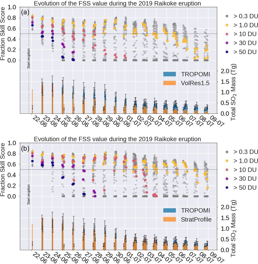
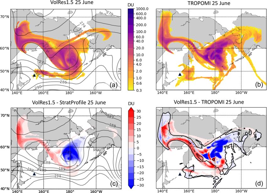
10862        J. de Leeuw et al.: SO2 dispersion model simulations and satellite retrievals for the 2019 Raikoke eruption

23 June. For the cloud layers at higher altitudes within the      overestimation of the spread of the cloud in NAME is even
stratosphere, the main wind direction was more zonal, re-         larger (not shown here).
sulting in the observed split in Fig. 3. The VolRes1.5 and
the StratProfile simulations show the same spatial pattern but    3.2   Fractional skill score (FSS)
have different SO2 VCDs within the cloud (see e.g. Fig. 3d).
The StratProfile (Fig. 3c) simulation shows a better agree-       The VolRes1.5 and the StratProfile simulations are gener-
ment with the TROPOMI SO2 VCD values for this day,                ally able to capture the large-scale structure of the SO2
which is expected based on its derivation.                        cloud, but differences between the simulations and the satel-
   By 25 June 2019, a large part of the cloud moves in a          lite retrievals occur after 4–5 d of simulation (see for exam-
north-western direction, spreading over the Asian continent       ple Fig. 6). To determine the timescales for which the sim-
as seen in Fig. 6a and b for both the VolRes1.5 simulation        ulations show skill compared to the TROPOMI retrievals,
and TROPOMI. Due to the variation in emission heights be-         we calculate the FSS score for each individual overpass for
tween the VolRes1.5 and the StratProfile simulations (Fig. 2),    a range of SO2 VCD contours (ranging between 0.3 and
we can identify the parts of the cloud in the NAME simula-        100 DU). The results for the smallest neighbourhood size
tions that are mainly within the troposphere and the strato-      N = 1 (i.e. the NAME output grid box size 0.2◦ latitude and
sphere by comparing their differences. The results are shown      0.4◦ longitude) are shown in Fig. 8 for (a) the VolRes1.5 and
in Fig. 6c, which shows that the north-western part of the        (b) the StratProfile simulation.
cloud is mainly within the troposphere, while the strato-            The VolRes1.5 simulation is able to capture the over-
spheric parts of the cloud remain centred around the low-         all outline of the cloud well for this period but struggles
pressure system. Calculating the difference between the Vol-      to simulate the peak SO2 VCD values within the retrieved
Res1.5 simulation and the TROPOMI retrievals in Fig. 6d,          TROPOMI SO2 cloud. Focussing on the SO2 VCD > 1 DU
we find that the pattern is very similar to Fig. 6c. This shows   points in Fig. 8a, the simulation has skill (FSS > 0.5) for up
that the VolRes1.5 simulation mainly overestimates the SO2        to 12.5 d after the eruption onset. This shows that the simula-
mass of the cloud in the troposphere and underestimates the       tion captures the overall dispersion of the cloud well, as it is
stratospheric part of the cloud.                                  able to distinguish between areas with and without any SO2
   On 27 June 2019, the SO2 cloud starts to spread also           across the NH. For SO2 VCDs greater than 30 DU, which
at higher altitudes, leading to a complex spatial pattern as      correspond to small-scale features within the volcanic cloud,
shown in Fig. 7. While the large-scale structure of the cloud     the simulation has no significant skill beyond 2.5 d after the
on 27 June has become much more complex, both the Vol-            start of the eruption. This agrees with the fact that the Vol-
Res1.5 and the StratProfile simulations capture the general       Res1.5 simulation was not able to capture the peak values on
SO2 VCD structure of the retrieved TROPOMI cloud well.            the 25 June 2019 observed by TROPOMI as shown in Fig. 6.
Note that the small-scale eddies observed by TROPOMI in              The FSS values for the StratProfile simulation (Fig. 8b)
the centre of the cloud are not simulated by NAME as a re-        reveal that this simulation performs better than VolRes1.5
sult of the limited (spatial and temporal) resolution of the      and has skill on a longer timescale for all of the SO2 VCDs.
NWP input. Therefore, the small-scale variability cannot be       For the lower SO2 VCDs (< 1 DU), the StratProfile simula-
captured by the model but instead is parameterised by the         tion remains skilful 2 d longer than the VolRes1.5 simulation
diffusion parameters as a random perturbation on the wind         (12.5 d versus 14.5 d). For the SO2 VCDs above 30 DU, the
field (see Sect. 2.3.1). This results in the spreading of the     FSS skill timescale has doubled compared to the VolRes1.5
SO2 cloud with a smoother pattern in the NAME simula-             simulation, showing again the importance of the emission
tions without the high peak values. This also explains the        profile on the skill of the simulation.
patchy variations shown in Fig. 6b and c within the cen-             The timescales for which the NAME simulations show
tre of the cloud. Averaging the SO2 VCDs over the whole           skill (compared to the TROPOMI retrievals) in terms of FSS
domain shown in Fig. 7 (thereby removing the small-scale          are shown in Fig. 9 and Table A1. Independent of the neigh-
features from TROPOMI), the average SO2 VCD values for            bourhood size, the StratProfile simulation has the highest
the VolRes1.5 simulation are 20 % lower than measured by          skill for all SO2 VCDs. Figure 9 shows that the StratPro-
TROPOMI. This is also evident from the dominant blue              file simulation is skilful on timescales twice as long for SO2
colours in Fig. 7b. For the StratProfile simulation (Fig. 7c)     VCD values above 10 DU compared to the VolRes1.5 and
the domain-average mass is within 0.01 Tg of SO2 of the           VolRes2.0 simulations. Interestingly the change in neigh-
TROPOMI SO2 mass estimate (i.e. StratProfile SO2 mass es-         bourhood size (i.e. averaging region) has only a limited im-
timate is < 1 % lower than TROPOMI).                              pact on the skill timescales for low SO2 VCDs (below 5 DU).
   Finally, we also find a larger spread of the cloud in both     This shows that all of the simulations are able to capture
the VolRes1.5 and StratProfile simulations as seen in Fig. 7b     the horizontal extent of the SO2 cloud well on spatial scales
and c by the red values outside the 1 DU TROPOMI contour.         similar to our smallest output grid used (0.2◦ × 0.4◦ ) and on
We only included the values > 1 DU in this plot for clarity       timescales of 2–3 weeks after the start of the eruption.
of the figure. When including lower values (0.3–1 DU), the

Atmos. Chem. Phys., 21, 10851–10879, 2021                                         https://doi.org/10.5194/acp-21-10851-2021
You can also read