The future sea-level contribution of the Greenland ice sheet: a multi-model ensemble study of ISMIP6 - AWI
←
→
Page content transcription
If your browser does not render page correctly, please read the page content below
The Cryosphere, 14, 3071–3096, 2020
https://doi.org/10.5194/tc-14-3071-2020
© Author(s) 2020. This work is distributed under
the Creative Commons Attribution 4.0 License.

The future sea-level contribution of the Greenland ice sheet: a
multi-model ensemble study of ISMIP6
Heiko Goelzer1,2,32 , Sophie Nowicki3 , Anthony Payne4 , Eric Larour5 , Helene Seroussi5 , William H. Lipscomb6 ,
Jonathan Gregory7,8 , Ayako Abe-Ouchi9 , Andrew Shepherd10 , Erika Simon3 , Cécile Agosta11 , Patrick Alexander12,13 ,
Andy Aschwanden14 , Alice Barthel15 , Reinhard Calov16 , Christopher Chambers17 , Youngmin Choi18,5 ,
Joshua Cuzzone18 , Christophe Dumas11 , Tamsin Edwards19 , Denis Felikson3 , Xavier Fettweis20 ,
Nicholas R. Golledge21 , Ralf Greve17,22 , Angelika Humbert23,24 , Philippe Huybrechts25 , Sebastien Le clec’h25 ,
Victoria Lee4 , Gunter Leguy6 , Chris Little26 , Daniel P. Lowry27 , Mathieu Morlighem18 , Isabel Nias3,28,33 ,
Aurelien Quiquet11 , Martin Rückamp23 , Nicole-Jeanne Schlegel5 , Donald A. Slater29,34 , Robin S. Smith7 ,
Fiamma Straneo29 , Lev Tarasov30 , Roderik van de Wal1,31 , and Michiel van den Broeke1
1 Institute for Marine and Atmospheric research Utrecht, Utrecht University, Utrecht, the Netherlands
2 Laboratoire   de Glaciologie, Université Libre de Bruxelles, Brussels, Belgium
3 Cryospheric Sciences Laboratory, Goddard Space Flight Center, NASA, Greenbelt, MD 20771, USA
4 Centre for Polar Observation and Modelling, School of Geographical Sciences, University of Bristol, Bristol, UK
5 Jet Propulsion Laboratory, California Institute of Technology, Pasadena, CA 91109, USA
6 Climate and Global Dynamics Laboratory, National Center for Atmospheric Research, Boulder, CO 80305, USA
7 National Centre for Atmospheric Science, University of Reading, Reading, UK
8 Met Office, Hadley Centre, Exeter, UK
9 Atmosphere and Ocean Research Institute, The University of Tokyo, Kashiwa-shi, Chiba 277-8564, Japan
10 Centre for Polar Observation and Modelling, University of Leeds, Leeds, LS2 9JT, UK
11 Laboratoire des Sciences du Climat et de l’Environnement, LSCE/IPSL, CEA-CNRS-UVSQ, Université Paris-Saclay,

91191 Gif-sur-Yvette, France
12 Lamont-Doherty Earth Observatory, Columbia University, Palisades, NY 10964, USA
13 NASA Goddard Institute for Space Studies, New York, NY 10025, USA
14 Geophysical Institute, University of Alaska, Fairbanks, AK 99775, USA
15 Los Alamos National Laboratory, Los Alamos, NM 87545, USA
16 Potsdam Institute for Climate Impact Research, Potsdam, Germany
17 Institute of Low Temperature Science, Hokkaido University, Sapporo, Japan
18 Department of Earth System Science, University of California Irvine, CA 92697, USA
19 Department of Geography, King’s College London, London, UK
20 Laboratory of Climatology, Department of Geography, SPHERES research unit, University of Liège, Liège, Belgium
21 Antarctic Research Centre, Victoria University of Wellington, Wellington, New Zealand
22 Arctic Research Center, Hokkaido University, Sapporo, Japan
23 Alfred-Wegener-Institut Helmholtz-Zentrum für Polar- und Meeresforschung, Bremerhaven, Germany
24 Faculty of Geosciences, University of Bremen, Bremen, Germany
25 Earth System Science & Departement Geografie, Vrije Universiteit Brussel, Brussels, Belgium
26 Atmospheric and Environmental Research, Inc., Lexington, MA 02421, USA
27 GNS Science, Lower Hutt, New Zealand
28 Earth System Science Interdisciplinary Center, University of Maryland, College Park, MD 20740, USA
29 Scripps Institution of Oceanography, University of California San Diego, La Jolla, CA 92037, USA
30 Dept of Physics and Physical Oceanography, Memorial University of Newfoundland, Canada
31 Geosciences, Physical Geography, Utrecht University, Utrecht, the Netherlands
32 NORCE Norwegian Research Centre, Bjerknes Centre for Climate Research, Bergen, Norway
33 Department of Geography and Planning, School of Environmental Sciences, University of Liverpool, Liverpool, UK

Published by Copernicus Publications on behalf of the European Geosciences Union.
3072                                                              H. Goelzer et al.: Multi-model ensemble study of ISMIP6

34 School   of Geography and Sustainable Development, University of St Andrews, St Andrews, UK

Correspondence: Heiko Goelzer (heig@norceresearch.no)

Received: 24 December 2019 – Discussion started: 21 January 2020
Revised: 16 June 2020 – Accepted: 2 July 2020 – Published: 17 September 2020

Abstract. The Greenland ice sheet is one of the largest con-      bution are systematically organized for the entire global ice
tributors to global mean sea-level rise today and is expected     sheet modelling community, extending earlier initiatives that
to continue to lose mass as the Arctic continues to warm.         were separated between the USA (SeaRISE, http://websrv.
The two predominant mass loss mechanisms are increased            cs.umt.edu/isis/index.php/SeaRISE_Assessment, last access:
surface meltwater run-off and mass loss associated with the       15 August 2020) and Europe (ice2sea, https://www.ice2sea.
retreat of marine-terminating outlet glaciers. In this paper we   eu, last access: 15 August 2020). In addition to the actual
use a large ensemble of Greenland ice sheet models forced         projections, the less tangible but equally important achieve-
by output from a representative subset of the Coupled Model       ment of ISMIP6 is the building of a community and the cre-
Intercomparison Project (CMIP5) global climate models to          ation and design of an intercomparison infrastructure that has
project ice sheet changes and sea-level rise contributions over   not existed before. The link with CMIP illustrates the ambi-
the 21st century. The simulations are part of the Ice Sheet       tion to bring community ice sheet model projections to the
Model Intercomparison Project for CMIP6 (ISMIP6). We es-          level of existing initiatives, e.g. in the field of coupled cli-
timate the sea-level contribution together with uncertainties     mate model simulations (Eyring et al., 2016). The project
due to future climate forcing, ice sheet model formulations       output and timeline are oriented towards providing input for
and ocean forcing for the two greenhouse gas concentration        the sixth assessment cycle of the Intergovernmental Panel on
scenarios RCP8.5 and RCP2.6. The results indicate that the        Climate Change (IPCC), where earlier assessments (Church
Greenland ice sheet will continue to lose mass in both scenar-    et al., 2013; Oppenheimer et al., 2019) had to rely on input
ios until 2100, with contributions of 90 ± 50 and 32 ± 17 mm      from various sources to provide ice sheet sea-level change
to sea-level rise for RCP8.5 and RCP2.6, respectively. The        projections. The present results are complemented by an-
largest mass loss is expected from the south-west of Green-       other paper on Antarctic ice sheet projections (Seroussi et
land, which is governed by surface mass balance changes,          al., 2020).
continuing what is already observed today. Because the con-          The overall mass balance of the GrIS is governed by the
tributions are calculated against an unforced control exper-      surface mass balance (SMB) that determines the amount of
iment, these numbers do not include any committed mass            mass that is added by snow accumulation and removed by
loss, i.e. mass loss that would occur over the coming cen-        meltwater run-off and sublimation and by the amount of mass
tury if the climate forcing remained constant. Under RCP8.5       that is lost through a large number of marine-terminating out-
forcing, ice sheet model uncertainty explains an ensemble         let glaciers. Over the period 1992–2018, the ice sheet has lost
spread of 40 mm, while climate model uncertainty and ocean        mass at an average rate of ∼ 140 Gt yr−1 , which is equiva-
forcing uncertainty account for a spread of 36 and 19 mm,         lent to a sea-level contribution of ∼ 0.4 mm yr−1 (The IM-
respectively. Apart from those formally derived uncertainty       BIE Team, 2019). The contribution of SMB-related changes
ranges, the largest gap in our knowledge is about the physi-      to these figures is ∼ 52 %, with the remaining 48 % being due
cal understanding and implementation of the calving process,      to increased discharge of outlet glaciers (The IMBIE Team,
i.e. the interaction of the ice sheet with the ocean.             2019).
                                                                     Process-based future ice sheet projections rely on numer-
                                                                  ical models that simulate the gravity-driven flow of ice un-
                                                                  der a given environmental forcing, subject to boundary con-
1   Introduction                                                  ditions at the surface, base and at the lateral boundaries. In
                                                                  our stand-alone modelling approach that connects to CMIP,
The aim of this paper is to estimate the contribution of
                                                                  the atmospheric and oceanic forcing is derived from CMIP
the Greenland ice sheet (GrIS) to future sea-level rise un-
                                                                  Global Climate Model (GCM) output.
til 2100 and the uncertainties associated with such projec-
                                                                     This work continues from an earlier ISMIP6 project
tions. The work builds on a worldwide community effort of
                                                                  (initMIP-Greenland; Goelzer et al., 2018) that compared the
ice sheet modelling groups that are organized in the frame-
                                                                  initialization techniques used by different ice sheet mod-
work of the Ice Sheet Model Intercomparison Project for
                                                                  elling groups. In many cases, the ice sheet projections pre-
CMIP6 (ISMIP6), which is endorsed by the Coupled Model
                                                                  sented here are directly based on modelling work that entered
Intercomparison Project (CMIP6). This is the first time that
                                                                  that earlier comparison. Differences between ice sheet mod-
process-based projections of the ice sheet sea-level contri-

The Cryosphere, 14, 3071–3096, 2020                                                  https://doi.org/10.5194/tc-14-3071-2020
H. Goelzer et al.: Multi-model ensemble study of ISMIP6                                                                      3073

els and, in particular, different ways of using the models are     spin-up techniques or steady-state assumptions at some ear-
a large source of uncertainty (Goelzer et al., 2018). The spe-     lier stage of the ice sheet history or hybrid approaches that
cific contribution of the present analysis to the range of ex-     combine features of optimization and spin-up (e.g. Pollard
isting future sea-level change projections lies therefore in the   and DeConto, 2012). See Goelzer et al. (2017, 2018) for a
quantification of ice sheet model (ISM) uncertainty, which is      comparison and an overview of different initialization strate-
done here for the first time in a consistent framework.            gies currently used in the ice sheet modelling community.
   In the following we discuss the approach and experimental          The experimental set-up of the initialization and the his-
set-up in Sect. 2 and briefly present the participating models     torical experiment leading up to the projections is left free
in Sect. 3. We analyse the modelled initial state (Sect. 4.1),     to be decided by the modellers (see Appendix A). The only
the 21st-century projections (Sect. 4.2) and associated uncer-     requirement is that the model state at the end of the historical
tainties (Sect. 4.3) and close with a discussion and conclu-       run should represent the state of the GrIS at the end of 2014
sions (Sect. 5). The two appendices give more detailed infor-      as a starting point for future projections. This time frame is
mation about the participating models (Appendix A) and list        set by CMIP6 requirements (Eyring et al., 2016). The length
the model results (Appendix B).                                    of the historical runs will consequently differ based on the
                                                                   initialization strategy of each individual model.
                                                                      Being an officially endorsed sub-project of CMIP6, the ex-
2   Approach and experimental set-up                               perimental design of ISMIP6 projections builds heavily on
                                                                   output of CMIP GCMs that are used to produce the forcing
In this section we describe the approach and experimen-            for ice sheet models over the 21st century. While ISMIP6 has
tal set-up for GrIS sea-level change projections performed         proposed ice sheet model projections based on CMIP6 GCM
within the framework of ISMIP6. While focused on the sci-          output as part of its extended experimental design (Now-
entific aims described in the introduction, the experimental       icki et al., 2020), the results discussed in this paper focus
framework is designed to be inclusive to a wide number of          solely on CMIP5-based forcing. Working with CMIP5 output
modelling approaches. We allow modelling groups to partic-         has allowed us to select GCMs from a well-defined ensem-
ipate with more than one submission to explore modelling           ble and sample the CMIP5 ensemble range in a controlled
choices like different horizontal grid resolution or initializa-   way, while CMIP6 model results are still being produced.
tion techniques with the same model. We also accommodate           For the core experiments that are the main focus of this pa-
models from the same code base but used by different groups,       per, we have selected three CMIP5 GCMs that perform well
knowing that modelling decisions (e.g. the chosen initializa-      over the historical period and maximize the spread in future
tion strategy) can be more important for the results than the      projections of a number of key climate change metrics rel-
underlying numerical scheme. The result is a heterogeneous         evant for GrIS evolution (Barthel et al., 2020). Three addi-
set of ice sheet models that can be understood as an ensem-        tional CMIP5 GCMs were selected using the same principle
ble of opportunity. In the following we refer to each of the 21    to extend the ensemble. We use the two scenarios RCP8.5
individual submissions as a “model”, encompassing the code         and RCP2.6 to cover a wide range of possible future climate
base as well as the modelling decisions (parameter choices,        evolution scenarios with particular focus on RCP8.5 (see Ta-
applied approximations, initialization strategy).                  ble 1). Exploring other scenarios was deprioritized in favour
   The experimental design of ISMIP6-Greenland projec-             of a feasible workload for the ice sheet modellers and for
tions extends the protocol of earlier ISMIP6 initiatives (Now-     producing forcing data.
icki et al., 2016; Goelzer et al., 2018; Seroussi et al., 2019)       The GCM output is used to separately derive ice sheet
and is described in detail in a separate publication (Nowicki      model forcing for the interaction with the atmosphere and
et al., 2020). Here we only summarize the most important as-       the ocean.
pects and refer to detailed descriptions elsewhere. The actual        Interaction with the atmosphere is incorporated in the
ice sheet projections for the period 1 January 2015–31 De-         models by prescribing surface mass balance (and tempera-
cember 2100 are tightly defined in terms of forcing and how        ture) anomalies relative to the period 1960–1989, for which
to apply it, while the preceding ice sheet initialization and      the ice sheet is assumed to be in balance with the forcing
historical run are largely up to the individual modeller.          (e.g. Mouginot et al., 2019). The forcing is produced with
   Ice sheet model (ISM) initialization to the present-day         the regional climate model MAR version v3.9 (Fettweis et
state is a critical aspect of any future ice sheet projection      al., 2013, 2017) that locally downscales the GCM forcing to
(Goelzer et al., 2017, 2018). It consists of defining the prog-    the GrIS surface (Fig. 1a, b). We take into account changes
nostic model state with the overall aim here to represent the      in the SMB due to elevation changes using a parameteriza-
present-day dynamic state of the GrIS as well as possible.         tion based on MAR output for the same simulation (Nowicki
In some cases modellers may initialize to a recent state of        et al., 2020). In cases where the modelled initial ice sheet
the ice sheet during the satellite era for which a large num-      differs substantially from the observed, we remap the SMB
ber of detailed observations of velocity and ice thickness are     anomalies from the observed geometry to the modelled ge-
available. In other cases, the models may be initialized using

https://doi.org/10.5194/tc-14-3071-2020                                                 The Cryosphere, 14, 3071–3096, 2020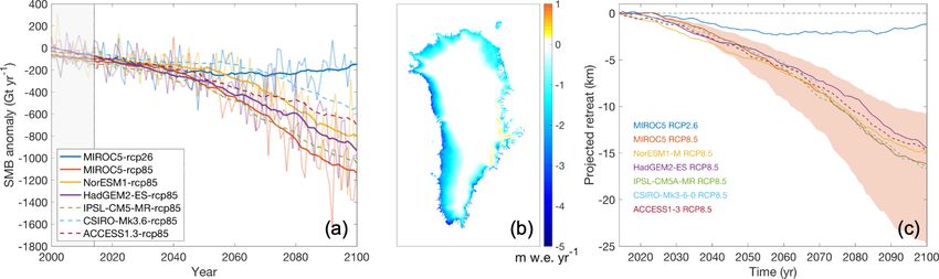
3074                                                                                                   H. Goelzer et al.: Multi-model ensemble study of ISMIP6

Table 1. List of GCM-forced experiments for ISMIP-Greenland projections. Climate model uncertainty is sampled with three core GCMs
and three additional extended GCMs. Two different scenarios (RCP8.5, RCP2.6) are evaluated for model MIROC5. Sensitivity to the ocean
forcing is sampled with three experiments under scenario RCP8.5. Forcing for the historical experiment is defined by each individual modeller
(not shown). Experiment “ctrl_proj” applies zero SMB anomalies, no SMB-height feedback and a fixed retreat mask (not shown).

   Exp ID                   exp05∗          exp06              exp07          exp08                 exp09           exp10          expa01         expa02        expa03
   GCM                      MIROC5          NorESM-M           MIROC5         HadGEM2-ES            MIROC5          MIROC5         IPSL-CM5A-MR   CSIRO-Mk3.6   ACCESS1-3
   RCP                      8.5             8.5                2.6            8.5                   8.5             8.5            8.5            8.5           8.5
   Ocean sensitivity        Medium          Medium             Medium         Medium                High            Low            Medium         Medium        Medium
  ∗ Experiments exp01–exp04 are open-framework experiments not listed here with the same GCM forcing as exp05–exp08. See text for details.

ometry using a technique developed specifically for that pur-                                          analysis. In a few models, the native grid is identical to the
pose (Goelzer et al., 2020b).                                                                          diagnostic grid. All results presented in this paper are based
   The standard approach for ocean forcing is based on                                                 on data on the common diagnostic grid.
an empirically derived retreat parameterization for tide-                                                 One of the main results presented below is the pro-
water glaciers (Slater et al., 2019, 2020) that is forced                                              jected sea-level contribution of the GrIS to 21st-century
by MAR run-off and ocean temperature changes in seven                                                  sea-level rise. In all cases, we calculate sea-level changes
drainage basins around Greenland. The forcing is illustrated                                           based on the evolving ice sheet geometry, taking into ac-
as Greenland-wide average of prescribed tidewater glacier                                              count the model specific densities for ice and sea wa-
retreat in Fig. 1c. In this retreat implementation, retreat and                                        ter and correcting for the map projection error following
advance of marine-terminating outlet glaciers in the ISMs are                                          Goelzer et al. (2020a). In agreement with the GlacierMIP ex-
prescribed as a yearly series of maximum ice front positions                                           ercise (http://www.climate-cryosphere.org/mips/glaciermip/
(Nowicki et al., 2020). This approach is a strong simplifica-                                          about-glaciermip, last access: 15 August 2020), we have
tion of the complex interaction between marine-terminating                                             attempted to remove the contribution of loosely connected
outlet glaciers and the ocean, for which physically based so-                                          glaciers and ice caps in the periphery of Greenland from our
lutions are in development but not available for all models.                                           mass change estimates to avoid double-counting in global
The retreat parameterization is designed to be used in the                                             sea-level change assessments. This has been done by cor-
wide variety of models under consideration. Uncertainty in                                             recting the ice sheet mass change per grid cell by the area
the parameterization is translated into a set of three ocean                                           fraction of the glaciers (level 0–1) in the Randolph Glacier
sensitivities (medium, high, low) covering the median, 75 %                                            Inventory (RGI Consortium, 2017). The assumed constant
and 25 % percentiles of sensitivity parameter κ that controls                                          ocean area for conversion from ice mass above flotation to
the amount of retreat given ocean temperature change and ice                                           sea-level equivalent (SLE) is 3.625×10¹⁴ m2 (Cogley, 2012;
sheet run-off (Slater et al., 2019, 2020). Results are explored                                        Gregory et al., 2019), which implies that 1 mm SLE equals
with the last two core experiments (Table 3).                                                          362.5 Gt ice mass. For cases where the model simulates iso-
   For some ISMs of high spatial resolution that incorpo-                                              static adjustment, we have assumed that corrections of the
rate a physical calving model, future evolution of marine-                                             ice mass above flotation due to bedrock changes are negligi-
terminating outlet glacier is alternatively forced directly by                                         ble on the centennial timescale (Goelzer et al., 2020a). All
changes in ocean temperature and run-off derived from the                                              sea-level contributions are corrected for model drift by sub-
GCM and Regional Climate Model (RCM) output (Slater et                                                 tracting the sea-level contribution from a control experiment
al., 2020). Simulations performed with this submarine melt                                             (ctrl_proj) and are therefore relative to the year 2014. This
implementation are considered as a contribution to the open                                            correction implies that the reported numbers have to be in-
framework of the exercise, designed to allow exploration of                                            terpreted as the ice sheet response to future forcing in addi-
novel modelling techniques that cannot be implemented in                                               tion to a background evolution that arises from forcing before
all models. We have decided to include model results from                                              2014, sometimes called the committed sea-level contribution
this open framework in our main analysis since they repre-                                             (e.g. Price et al., 2011). This committed contribution is ex-
sent a source of additional uncertainty in the way the forcing                                         pected to be positive for Greenland but much lower than the
is applied. For this group of models, the last two experiments                                         observed trend before 2014 (The IMBIE team, 2019) because
that sample uncertainty due to ocean forcing are not defined                                           the mass loss rate rapidly decreases in absence of additional
(Table 3).                                                                                             forcing (Price et al., 2011). For ensemble statistics we report
   Model output for the ISMIP6 experiments is initially pro-                                           mean (µ) and the 2× standard deviation (2σ ) range to quan-
duced by the participating groups on the individual native                                             tify the uncertainty unless stated differently in the text.
grid of their models, then conservatively interpolated to a
standard regular grid with a resolution close to the native grid
for submission to our archive and finally conservatively inter-
polated to a common 5 km × 5 km regular diagnostic grid for

The Cryosphere, 14, 3071–3096, 2020                                                                                                  https://doi.org/10.5194/tc-14-3071-2020
H. Goelzer et al.: Multi-model ensemble study of ISMIP6                                                                              3075

Figure 1. Illustration of atmospheric and oceanic forcing. (a) Greenland-wide SMB anomaly for projections starting at 2015. Strong lines
are 10-year running mean values for the core experiments (solid) and extended CMIP5 experiments (dashed), plotted over the full time series
in the background (omitted for the extended experiments for clarity). (b) spatial pattern of the average MIROC5-RCP8.5 SMB anomaly for
the period 2091–2100. (c) Greenland-wide average of prescribed tidewater glacier retreat (Slater et al., 2019, 2020). The shading gives the
range of ocean sensitivity sampled with two more experiments in MIROC5-RCP8.5-high and MIROC5-RCP8.5-low.

3   Participating groups and models                                     4     Results

We have 21 submissions from 14 modelling groups, cover-                 In this section we first present ice sheet modelling results
ing a wide range of the global ice sheet modelling commu-               for the end of the historical run, forming the starting point
nity (Table 2). Compared to initMIP-Greenland (Goelzer et               of sea-level change projections over the 21st century. This is
al., 2018) the number of participating modelling groups has             followed by the results of the projections, with a focus on the
slightly decreased with some removals and some new addi-                GrIS sea-level contribution and associated uncertainties.
tions, but the range of represented models is still broad. A
detailed description of the individual models and initializa-           4.1    Historical run and initial state
tion techniques is given in Appendix A together with a table
of important model characteristics (Table 4). The total range           The initial model states at the end of 2014 differ among the
of horizontal grid resolution is between 0.2 and 30 km, where           models in the ensemble as a result of different initialization
extreme values come from finite element models with adap-               strategies, forcing and parameter choices. Figure 2 illustrates
tive grid resolution that have high resolution near the margins         the diversity of modelled initial ice sheet area by showing the
to resolve narrow outlet glaciers and low resolution inland.            sum of grounded ice coverage across the ensemble. Disagree-
All participating models use either a form of data assimila-            ment in the periphery is partially related to a choice left de-
tion or nudging techniques of different degrees to improve              liberately to the individual modellers: which part of the ice-
the match with present-day observations (Table 4).                      covered area of Greenland should be modelled. While some
   All groups have contributed a complete set of core ex-               modellers target the entire observed ice-covered area, others
periments (Table 3), which form the basis of the analy-                 mask out unconnected or loosely connected glaciers, ice caps
sis for this paper. The submissions are identified by the               and ice fields in an attempt to avoid double-counting of those
group ID and model name (Table 2) and a counter to                      features in global assessments (see modelled ice masks for
distinguish several submissions from the same group (Ta-                individual models in Fig. S4 in the Supplement).
ble 3). Four models have used the non-standard open forc-                  Another view on the model spread for the initial state can
ing framework (BGC-BISICLES, UAF-PISM2, UCIJPL-                         be seen in Fig. 3, which shows the grounded ice area and
ISSM2, VUW-PISM), which does not define the ocean sensi-                grounded volume for all models in the ensemble. In com-
tivity experiments exp09 and exp10. In the BGC-BISICLES                 parison we show two different observed values that equally
case, they have been replaced by their own interpretation               depend on the choice of which part of the ice-covered area to
of high and low ocean forcing. The two models MUN-                      include in the estimate. This notably leads to a large range in
GSM1 and MUN-GSM2 have used remapped SMB anoma-                         area between a low estimate (main ice sheet; Rastner et al.,
lies (Goelzer et al., 2020b) to optimize the forcing for their          2012) and high estimate (all ice-covered area; Morlighem et
initial geometry, which differs more from the observations              al., 2017), while the volume difference is relatively small due
compared to other models.                                               to the limited thickness of peripheral glaciated areas. Com-
                                                                        pared to initMIP-Greenland (cf. Fig. 2 in Goelzer et al., 2018,
                                                                        but note the different-coloured map), the spread in initial
                                                                        states has been considerably reduced, which is partially re-

https://doi.org/10.5194/tc-14-3071-2020                                                        The Cryosphere, 14, 3071–3096, 2020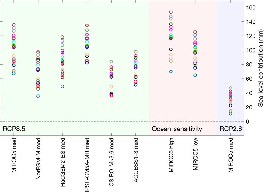
3076                                                                   H. Goelzer et al.: Multi-model ensemble study of ISMIP6

Table 2. Participants, modelling groups and ice sheet models in ISMIP6-Greenland projections.

        Contributors               Group ID     Model              Group
        Martin Rückamp,            AWI          ISSM               Alfred-Wegener-Institut Helmholtz-Zentrum für Polar- und
        Angelika Humbert                                           Meeresforschung, DE/University of Bremen, DE
        Victoria Lee,              BGC          BISICLES           Centre for Polar Observation and Modelling, School of Geo-
        Antony J. Payne,                                           graphical Sciences, University of Bristol, Bristol, UK
        Stephen Cornford,                                          Department of Geography, Swansea University, UK
        Daniel Martin                                              Computational Research Division, Lawrence Berkeley National
                                                                   Laboratory, California, USA
        Isabel J. Nias,            GSFC         ISSM               Cryospheric Sciences Laboratory, Goddard Space Flight Cen-
        Denis Felikson,                                            ter, NASA, USA
        Sophie Nowicki
        Ralf Greve,                ILTS_PIK     SICOPOLIS          Institute of Low Temperature Science, Hokkaido University,
        Reinhard Calov,                                            Sapporo, JP/Potsdam Institute for Climate Impact Research,
        Chris Chambers                                             Potsdam, DE
        Heiko Goelzer,             IMAU         IMAUICE            Utrecht University, Institute for Marine and Atmospheric re-
        Roderik van de Wal,                                        search (IMAU), Utrecht, NL
        Michiel van den Broeke
        Nicole-Jeanne              JPL          ISSM               Jet Propulsion Laboratory, California Institute of Technology,
        Schlegel,                                                  Pasadena, USA
        Helene Seroussi
        Joshua K. Cuzzone,         JPL          ISSM-PALEO         Jet Propulsion Laboratory, California Institute of Technology,
        Nicole-Jeanne Schlegel                                     Pasadena, USA
        Aurélien Quiquet,          LSCE         GRISLI             LSCE/IPSL, Laboratoire des Sciences du Climat et de
        Christophe Dumas                                           l’Environnement, CEA-CNRS-UVSQ, Gif-sur-Yvette, FR
        Lev Tarasov                MUN          GSM                Dept of Physics and Physical Oceanography, Memorial Univer-
                                                                   sity of Newfoundland, Canada
        William H. Lipscomb,       NCAR         CISM               National Center for Atmospheric Research, Boulder, USA
        Gunter Leguy
        Andy Aschwanden            UAF          PISM               Geophysical Institute, University of Alaska Fairbanks, USA
        Youngmin Choi,             UCI_JPL      ISSM               University of California Irvine, USA/
        Helene Seroussi,                                           Jet Propulsion Laboratory, California Institute of Technology,
        Mathieu Morlighem                                          Pasadena, USA
        Sébastien Le clec’h,       VUB          GISM               Vrije Universiteit Brussel, Brussels, BE
        Philippe Huybrechts,
        Dan Lowry,                 VUW          PISM               GNS Science, Lower Hutt, NZ/Antarctic Research Centre,
        Nicholas R. Golledge                                       Victoria University of Wellington, NZ

lated to ongoing improvements of the modelling techniques               loss during the historical period, but the magnitude often
of individual groups and partly because some extreme mod-               falls below the observed range. In some cases this discrep-
els are not part of the ensemble anymore.                               ancy is explained by the fact that the ice sheet is exposed to
   The initial model state at the end of 2014 is the result of          GCM forcing over the historical period which does not ex-
a model-specific initialization that includes a short historical        hibit the observed interannual and interdecadal variability. In
run. We display the ice mass evolution for this experiment              other cases, the historical run is not specifically forced, rather
followed by a standardized control experiment (ctrl_proj)               representing the background evolution arising as an artefact
for the same period as the projections but assuming zero                of the initialization. In any case, representing the historical
SMB anomalies and a fixed retreat mask from 2015 onwards                mass loss accurately was not a strong priority for our experi-
(Fig. 4). In most models the ice sheet experiences a mass

The Cryosphere, 14, 3071–3096, 2020                                                          https://doi.org/10.5194/tc-14-3071-2020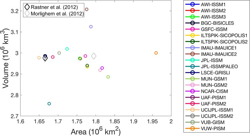
H. Goelzer et al.: Multi-model ensemble study of ISMIP6 3077
Table 3. Experiment overview. List of experiments that have been performed by the participating groups.
Core experiments Extensions
Exp ID historical ctrl_proj exp05 exp06 exp07 exp08 exp09 exp10 expa01 expa02 expa03
GCM – – MIROC5 NorESM MIROC5 HadGEM2-ES MIROC5 MIROC5 IPSL-CM5A-MR CSIRO-Mk3.6 ACCESS1-3
RCP – – 8.5 8.5 2.6 8.5 8.5 8.5 8.5 8.5 8.5
Sensitivity – – Medium Medium Medium Medium High Low Medium Medium Medium
AWI-ISSM1 x x x x x x x x x x x
AWI-ISSM2 x x x x x x x x x x x
AWI-ISSM3 x x x x x x x x x x x
BGC-BISICLES x x x1 x1 x1 x1 x1,2 x1,2 x1 x1 x1
GSFC-ISSM x x x x x x x x x x x
ILTSPIK- x x x x x x x x x x x
SICOPOLIS1
ILTSPIK- x x x x x x x x x x x
SICOPOLIS2
IMAU-IMAUICE1 x x x x x x x x – – –
IMAU-IMAUICE2 x x x x x x x x x x x
JPL-ISSM x x x x x x x x x x x
JPL-ISSMPALEO x x x x x x x x – – –
LSCE-GRISLI x x x x x x x x x x x
MUN-GSM1 x x x x x x x x – – –
MUN-GSM2 x x x x x x x x x x x
NCAR-CISM x x x x x x x x x x x
UAF-PISM1 x x x x x x x x x x x
UAF-PISM2 x x x1 x1 x1 x1 – – x1 x1 x1
UCIJPL-ISSM1 x x x x x x x x x x x
UCIJPL-ISSM2 x x x1 x1 x1 x1 – – – – –
VUB-GISM x x x x x x x x x x x
VUW-PISM x x x1 x1 x1 x1 – – – – –
1 Open format not using the retreat parameterization. 2 Own strategy to produce high and low ocean forcing.
Figure 3. Grounded ice area and grounded volume for all models
(circles). Observed values (Morlighem et al., 2017) are given for
the entire ice-covered region (light-grey diamond) and for the re-
gion of the main ice sheet (black diamond) where loosely connected
glaciers and ice caps are removed (Rastner et al., 2012).
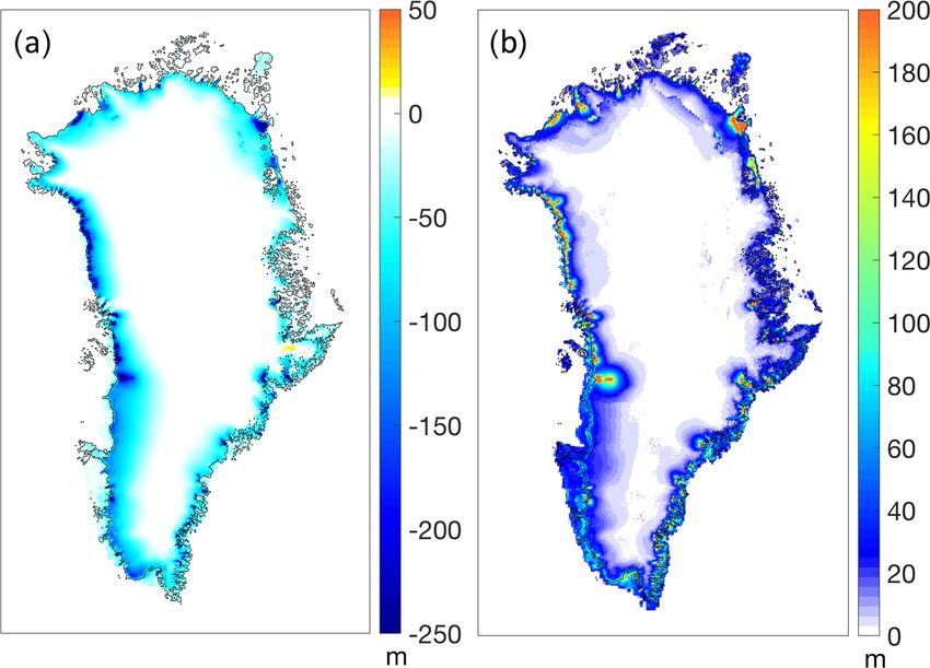
Figure 2. Common initial ice mask of the ensemble of models in the The control experiment (ctrl_proj) is in most cases the re-
intercomparison. The colour code indicates the number of models sult of competing tendencies to (1) continue the mass trend
(out of 21 in total) that simulate ice at a given location. Outlines
before 2014 and (2) relax toward an unforced state as a re-
of the observed main ice sheet (Rastner et al., 2012) and all ice-
covered regions (i.e. main ice sheet plus small ice caps and glaciers;
sult of removing the anomalies at the start of the projection
Morlighem et al., 2017) are given as black and grey contour lines, period in 2015. The ensemble range of sea-level contribution
respectively. A complete set of figures displaying individual model due to that drift in experiment ctrl_proj is −50 to 15 mm
results is given in the Supplement. (Table B1).
We further evaluate the initial model state at the end of
2014 in comparison to ice-sheet-wide observational datasets
mental set-up, where any background evolution is effectively (Fig. 5). We calculate the root mean square error (RMSE)
removed by subtracting results of experiment ctrl_proj. of the modelled data compared to observations of ice thick-
https://doi.org/10.5194/tc-14-3071-2020 The Cryosphere, 14, 3071–3096, 2020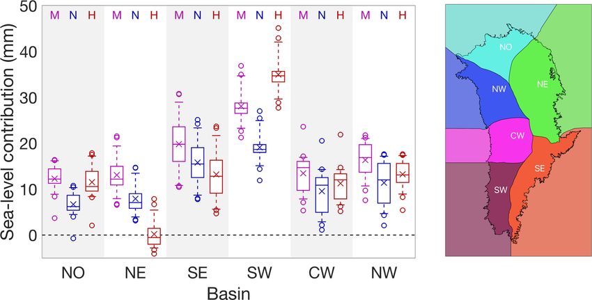
3078                                                                  H. Goelzer et al.: Multi-model ensemble study of ISMIP6

                                                                      ment of the ice sheet model geometry or surface velocity
                                                                      with observations can go hand in hand with a large drift in
                                                                      the control experiment (Fig. 5d), which may indicate too
                                                                      short of a relaxation during initialization. Similarly, modi-
                                                                      fying the applied background SMB forcing can be used to
                                                                      reduce mismatch with the observed velocity and geometry.
                                                                      Finally, masking operations can be used to constrain the ice
                                                                      sheet model area and consequently the geometry, reducing
                                                                      the prognostic capabilities of the model. Combining comple-
                                                                      mentary metrics and auxiliary information should be used in
                                                                      model ranking and weighting attempts. Another aspect that
                                                                      would have to be carefully considered for model weighting
                                                                      for ensemble statistics is the fact that several models have
                                                                      strong similarities and their results may therefore be over-
Figure 4. Ice mass change relative to the year 2014 for the histor-   represented in the ensemble.
ical run and experiment ctrl_proj. The colour scheme is the same
as in Fig. 3. Recent reconstructions of historical mass change (The
IMBIE Team, 2019) are given as a dotted grey line with cumulated      4.2   Projections
uncertainties assuming fully correlated and uncorrelated errors in
light and dark shading, respectively. The dashed black-and-white
line shows one specific reconstruction going back longer in time      In the following we first present sea-level projections for the
(Mouginot et al., 2019).                                              four core experiments with medium ocean forcing sensitiv-
                                                                      ity. Results of the projection experiments (2015–2100) are
                                                                      always presented relative to a control experiment (ctrl_proj)
ness (Morlighem et al., 2017) and horizontal surface velocity         with a focus on MIROC5-forced experiments, which shows
magnitude (Joughin et al., 2016). The diagnostics are calcu-          the strongest warming among the three selected GCMs. The
lated for subsampled data to reduce spatial correlation in the        ensemble mean ice thickness changes for scenario MIROC5-
error estimates, and we show median values for different off-         RCP8.5 shows a strong thinning at the margin due to the
sets. The comparison shows a wide diversity of the models             effect of increased surface meltwater run-off and marine-
in terms of their match with the observed ice thickness dis-          terminated glacier retreat (Fig. 6a). The strongest response
tribution (Fig. 5a) and velocity (Fig. 5b). We include a com-         is seen at the marine margins where both effects combine to
parison with the logarithm of the velocity magnitude (nor-            a thinning of up to several hundred metres, while the interior
malized by 1 m yr−1 ), which reduces the emphasis of errors           of the ice sheet is thickening less than 10 m in response to
in high velocities at the margins (Fig. 5c). These diagnostics        increased snow accumulation, except for some places in the
are complemented by the absolute ice thickness change in              south-east, where the thickening can reach 20 m and more.
ctrl_proj that serves as a measure of the model drift (Fig. 5d).         The spread in the projections due to ice sheet model un-
The largest thickness errors arise for coarse-resolution mod-         certainty and its spatial distribution is illustrated in Fig. 6b,
els that show substantial mismatches in particular at (but not        showing the ensemble standard deviation for experiment
limited to) the ice sheet margins. These are also models that         MIROC5-RCP8.5. The regions of largest uncertainty overlap
do not apply calibration techniques to optimize the geome-            with the regions of largest thinning due to differences in the
try during initialization. Some of the models with the low-           response of tidewater glaciers and their precise location in
est RMSE for ice thickness (e.g. LSCE-GRISLI and UAF-                 different models. The response to the anomalous SMB forc-
PISM) show relatively large errors in velocity, indicative of         ing is more homogeneous between models (cf. Fig. S8) as the
the prioritized field during optimization (thickness) and of          magnitude is largely prescribed and can mostly vary due to
the dependence between geometry and dynamic behaviour.                differences in ice masks across the ensemble. Exceptions are
Nevertheless, a few examples show that low errors in thick-           the remapped SMB anomalies (MUN-GSM1, MUN-GSM2)
ness and velocity are not mutually exclusive. See Figs. S3,           that are displaced to match the model geometry and height-
S4 and S5 for a visual comparison of individual models with           dependent SMB changes that are model specific, visible in
observations for ice thickness, surface elevation and velocity,       the north-east.
respectively.                                                            The sea-level contribution for MIROC5-RCP8.5 is
   While a formal ranking and weighting of the ice sheet              steadily increasing in all ice sheet models with an increas-
models based on the provided information is outside of the            ing rate of change until the end of the 21st century, indicative
scope of this paper, we caution that different evaluation met-        of accelerating mass loss for this very high emission scenario
rics should be combined and balanced in that case. This has           (Fig. 7b). Short-term variability in this diagnostic is mainly
already been mentioned for the comparison of errors in ice            due to interannual variability in the applied SMB forcing and
thickness and velocity. Another example is that good agree-           therefore synchronized across the ensemble. The average rate

The Cryosphere, 14, 3071–3096, 2020                                                       https://doi.org/10.5194/tc-14-3071-2020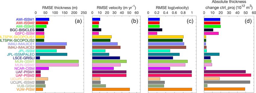
H. Goelzer et al.: Multi-model ensemble study of ISMIP6 3079
Figure 5. (a–c) Error estimate of model output at the end of the historical run compared to observations. (a) Root mean square error (RMSE)
of ice thickness compared to observations (Morlighem et al., 2017). RMSE of the horizontal velocity magnitude (b) and the logarithm
of the horizontal velocity magnitude (c) compared to observations (Joughin et al., 2016). The diagnostics have been calculated for grid
cells subsampled regularly in space to reduce spatial correlation; we show median values for different possible offsets of this sampling.
(d) Absolute thickness change in experiment ctrl_proj integrated over the model grid.
Differences in results between individual ice sheet mod-
els are not easily linked to general ice sheet model charac-
teristics (e.g. resolution, approximation to the force balance,
treatment of basal sliding), and the relatively small ensemble
size prevents us from applying statistical approaches to do
so. Nevertheless, a few notable differences can be mentioned.
Models using the open framework overall show lower contri-
butions compared to models using the standard retreat forc-
ing, although they are not clear outliers in the range of pro-
jections. Results from the two groups that have applied both
approaches in parallel confirm this conclusion (see Table 5).
For example, RCP8.5 results from models using the open ap-
proach (n = 4) are on average 23 mm lower compared to re-
sults under standard forcing. Focussing on the latter group
(standard forcing), models with larger initial area and vol-
Figure 6. Ensemble mean (a) and standard deviation (b) of ice ume tend to produce larger sea-level contributions. This is the
thickness change in MIROC5-RCP8.5 minus control over the 21st expected behaviour given the effect of both forcing mecha-
century. Thin black lines indicate the observed ice-covered area nisms: (1) a model of larger ice sheet extent will produce
(Morlighem et al., 2017). more run-off at the margins under the anomalous SMB forc-
ing; (2) thicker and more extended marine ice sheet margins
will lose more mass to the retreat parameterization.
of change across the ensemble is 0.9 and 2.4 mm yr−1 over The end members of the ensemble in terms of sea-level
the periods 2051–2060 and 2091–2100, respectively. contribution (IMAU-IMAUICE2: high; JPL-ISSMPALEO:
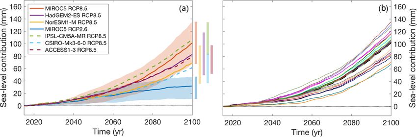
The total GrIS sea-level contribution by 2100 for low) are amongst the models with the lowest resolution in
MIROC5-RCP8.5 is projected between 67 and 135 mm, with the ensemble, which could suggest that low-resolution mod-
an ensemble mean (n = 21) and 2σ range of 101 ± 40 mm. els have larger uncertainty but not necessarily a bias. How-
In contrast, GCM MIROC5 forced under scenario RCP2.6 ever, note that the two lowest models (JPL-ISSMPALEO and
leads to a contribution of only 32 ± 17 mm, and forcing from VUW-PISM) did not apply the SMB-height feedback, which
the two other core GCMs for the RCP8.5 scenario lead to may explain some of the low response for these models.
contributions of 83 ± 37 and 69 ± 38 mm for HadGEM2-ES We can also compare results to a schematic experi-
and NorESM1, respectively (Fig. 7a). Detailed results for all ment where atmosphere and ocean forcing is applied to the
models and scenarios are given in Fig. 12 and listed in Ta- present-day ice sheet without any dynamical response (NO-
ble 5 in Appendix B. ISM, grey dashed line in Fig. 7b). The only exception is the
https://doi.org/10.5194/tc-14-3071-2020 The Cryosphere, 14, 3071–3096, 20203080 H. Goelzer et al.: Multi-model ensemble study of ISMIP6
Figure 7. Ensemble sea-level projections. (a) ISM ensemble mean projections for the core experiments (solid) and extended experiments
(dashed). The background shading gives the model spread for the two MIROC5 scenarios and is omitted for the other GCMs for clarity but
indicated by the bars on the right-hand side. (b) Model specific results for MIROC5-RCP8.5. The colour scheme is the same as in previous
figures. The dashed line is the result of applying the atmosphere and ocean forcing to the present-day ice sheet without any dynamical
response (NOISM).
SMB-height feedback that is propagated according to height larger-than-observed ice sheet model configurations (see in-
changes due to the applied SMB anomaly itself and due to set in Fig. 8).
local thinning at the margins where the retreat mask is ap- The results in Fig. 8 show the projected contribution to
plied. In this approach, biases in the initial state are reduced sea-level rise in the year 2100, indicating a north–south gra-
to measurement uncertainties, while dynamic changes are ig- dient with larger contributions from the south. The basin with
nored by construction. If the dynamic response of the ice the largest contributions is “SW” due to an extended ablation
sheet to the retreat mask forcing is expected to increase the zone in south-west Greenland, which is the region with the
mass loss, one could suggest that for the observed geome- largest source of sea-level contribution from changes in SMB
try and for a given forcing, NOISM should serve as a lower already observed (The IMBIE Team, 2019; Mouginot et al.,
bound to a “perfect” projection in our standard framework. 2019). However, note for this comparison that the basins do
Because NOISM currently tracks the ensemble mean of the not all have the same area. When we interpret the ensemble
projections, the argument could be extended to suggest that standard deviation relative to the ensemble mean as a mea-
taking the model mean for the best guess could imply a low sure for ice sheet model uncertainty, the largest uncertainty of
bias. ∼ 40 % is present in the “NO” and “SE” basins and the lowest
We do not have a dedicated core experiment to separate uncertainty of 17 % in the “SW” basin. The good agreement
the effect of the parameterized SMB-height feedback from between models for “SW” can be explained by the domi-
the ensemble of models. But such analysis will be possible nance of the SMB forcing in this basin, which is prescribed
with some of the extended experiments that are in prepara- in our experiments, so that variations between models mainly
tion. If we were to rely on results of NOISM, the feedback occur due to differences in ice sheet mask.
accounts for 6 %–8 % of the total sea-level contribution in the Comparing results for RCP8.5 between the three GCMs
year 2100 for RCP8.5 experiments, confirming similar num- side by side (Fig. 8) shows that the SW basin has the low-
bers from earlier studies (Goelzer et al., 2013; Edwards et al., est ISM interquartile range in all cases but is also one of the
2014a, b). However, the NOISM figures are subject to small two basins (SW and NE) with the largest difference between
biases due to missing dynamic height changes that would, GCMs. While the large GCM difference in the SW can be
for example, thin the marine margins and relatively thicken explained by the GCM-specific warming pattern and their in-
land-terminated ice sheet margins that are steepening in these fluence on the SMB forcing, differences in the NE basin are
projections in response to the anomalous SMB forcing. governed mainly by the ocean forcing.
Ocean sensitivity
4.3 Uncertainty analysis
Uncertainty in the tidewater glacier retreat parameteriza-
In this section we analyse uncertainties in ice sheet response tion is sampled with three experiments under forcing sce-
due to ISM differences, forcing scenarios and GCM bound- nario MIROC5-RCP8.5. Results for the three experiments
ary conditions on a regional basis. We use an existing basin are again compared per region (Fig. 9). The largest impact of
delineation (IMBIE2-Rignot, Rignot et al., 2011) that sepa- differences in ocean forcing is visible in region CW, which
rates the ice sheet into six drainage basins, which has been is dominated by the response of Jakobshavn Isbrae, one of
extended outside the observed ice mask to accommodate the largest outlet glaciers in Greenland. In the SW region,
The Cryosphere, 14, 3071–3096, 2020 https://doi.org/10.5194/tc-14-3071-2020H. Goelzer et al.: Multi-model ensemble study of ISMIP6 3081
when selecting one out of six GCMs. For each of the three
RCP8.5 core experiments with medium ocean sensitivity,
the absolute 2σ range, indicative of the ISM uncertainty, is
∼ 40 mm (n = 21). For the extended experiments that have
not been performed with some of the high and low ex-
treme models, the absolute 2σ range is reduced at ∼ 30 mm
(n = 15). The 2σ range of the ISM means across the six
GCMs, indicative of the climate forcing uncertainty, is of
similar magnitude (36 mm) compared to the ISM uncertainty,
while the spread of the means for three different ocean sen-
sitivities is about half (19 mm), indicating the approximate
Figure 8. Regional analysis of ice sheet changes for the three core relative importance of the three sources of uncertainty. Note
GCMs (MIROC5–M, NorESM–N, HadGem2-ES–H) under sce- that the reported GCM uncertainty based on only six models
nario RCP8.5. The box plots show the ensemble median (line), does not represent the full CMIP ensemble range.
mean (cross), interquartile range (box), range (whiskers) and out-
liers (circles). The basin definition is based on the IMBIE2-Rignot 4.4 Ice dynamic contribution
delineation (Rignot et al., 2011).
In this section we give an impression of the role of atmo-
spheric and oceanic forcing and the contribution of ice dy-
namics. Separating the different forcing mechanisms com-
pletely requires dedicated single-forcing experiments that
have been proposed as part of the extended experiments in
the ISMIP6 protocol (Nowicki et al., 2020) but have not been
studied here. Such analysis exceeds the scope of this paper
and will be explored in a forthcoming publication.
To characterize the strength of the ocean forcing per re-
gion and forcing scenario, we have calculated the ice vol-
ume (in millimetres of sea-level equivalent) that would be in-
stantaneously removed by the retreat parameterization from
the observed ice sheet geometry (Fig. 10a). For an ice sheet
model, the actual mass loss due to the retreat parameteriza-
Figure 9. Regional analysis of uncertainty due to ocean forcing.
Ensemble mean sea-level contribution for MIROC5-RCP8.5 for low tion is considerably larger than the diagnostic shown here as
(green), medium (cyan) and high (blue) ocean forcing. The mean of the ice sheet responds dynamically to a retreat of the calv-
the total Greenland contribution is 97, 101 and 116 mm for low, ing front. The ice flow accelerates and transports more mass
medium and high ocean forcing, respectively. to the marine margin that is subsequently removed by the
masking, while the ice sheet is thinning further inland. This
dynamic and non-linear response is the reason why physi-
which is dominated by changes in SMB, differences in the cally based ice sheet models are indispensable to producing
ocean forcing have only a minor impact on the results, in ice sheet projections for any timescale longer than a decade
line with findings described above. The mean spread due to or 2. The diagnostic is contrasted by the integrated SMB
ocean forcing over all ISMs that have performed the experi- anomaly over the observed geometry (Fig. 10b), which rep-
ments (n = 18) is 19 mm when summed over all six regions resents the dominant forcing for the resulting total sea-level
to get the Greenland-wide contributions. contribution from the experiments (Fig. 10c). The SMB con-
Combining projected sea-level contributions of the GrIS tribution is again calculated using the NOISM approach de-
from all experiments, the ensemble mean and 2σ range scribed above, taking into account elevation changes arising
for CMIP5 RCP8.5 is 90 ± 50 mm (n = 144), including six from the SMB anomaly itself to propagate the parameterized
GCMs and three ocean sensitivities. The ensemble mean for SMB-elevation feedback. In this case, however, we omit the
RCP2.6 is 32 ± 17 mm (n = 21), sampling only one GCM tidewater glacier retreat in an atmosphere-only set-up.
(MIROC5) and one ocean sensitivity (medium). The cor- Visual inspection of the similarity between rows b and c
responding ratios σ/µ are 28 % for RCP8.5 and 27 % for suggests that the SMB anomaly is the governing forcing in
RCP2.6, respectively, indicating that the relative uncertainty our experiments, while oceanic forcing plays a more limited
depends weakly on the ensemble mean and ensemble size. role for the results. In line with results described above, basin
The ISM ensemble mean in experiment MIROC5-RCP8.5- “SW” shows the lowest relative importance of oceanic forc-
medium is 101 ± 40 mm (n = 21), with σ/µ = 20 %, mean- ing, and basin “NW” shows the largest.
ing that the relative uncertainty reduces by only one-third
https://doi.org/10.5194/tc-14-3071-2020 The Cryosphere, 14, 3071–3096, 20203082 H. Goelzer et al.: Multi-model ensemble study of ISMIP6
Figure 10. Ocean and atmospheric forcing and sea-level response. (a) Volume instantaneously removed by the prescribed tidewater glacier
retreat mask when applied to the observed geometry (Morlighem et al., 2017). (b) Integrated surface mass balance anomaly forcing over the
observed geometry. (c) Ensemble mean sea-level contribution for all models using the standard forcing approach. Bars in (a) and (c) are for
low and high ocean sensitivity. Note the different vertical scale for (a) compared to (b) and (c).
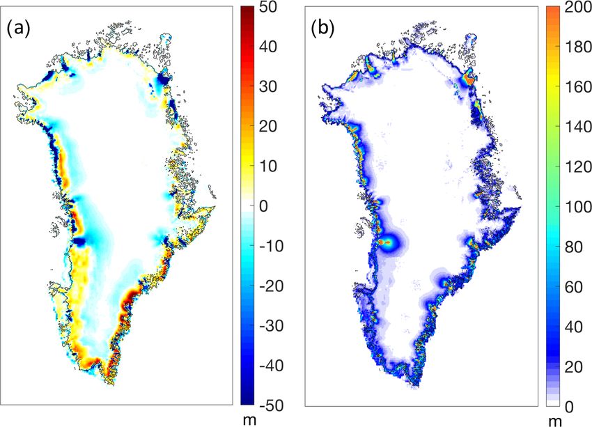
Figure 11 illustrates the role of ice dynamic changes in our
projections. We have calculated the mean dynamic contribu-
tion as the residual of the local mass change and the inte-
grated SMB anomaly (Fig. 11a) as well as the corresponding
standard deviation (Fig. 11b) for the ISM ensemble. Note that
this diagnostic includes all ice thickness changes that are not
explicitly related to SMB changes. The dynamic contribution
(Fig. 11a) shows large negative values in places where the
retreat parameterization has removed ice at the margins and
from connected inland regions that have been thinning in re-
sponse (which is therefore not explained by SMB changes).
A region of positive dynamic contribution is visible in the
land-terminated ablation zones around Greenland, where the
negative SMB anomaly steepens the margins, which is com-
pensated by dynamic thickening (Huybrechts and deWolde,
1999). Further inland, the corresponding upstream thinning Figure 11. Dynamic contribution for experiment MIROC5-RCP8.5.
is visible as a negative dynamic signal. The largest differ- (a) Ensemble mean dynamic ice thickness change residual and
ences between models are located in regions of tidewater (b) standard deviation. See Fig. S9 in the Supplement for patterns
glacier retreat, where the amount of ice available for calv- for each individual model.
ing varies between models due to inaccuracies in the initial
state.
The results indicate that the GrIS will continue to lose mass
in both scenarios until 2100, with contributions of 90 ± 50
5 Discussion and conclusion and 32 ± 17 mm to sea-level rise for RCP8.5 and RCP2.6,
respectively.
In the previous sections we have presented sea-level change Our estimates are around 10 mm lower compared to GrIS
projections for the GrIS over the 21st century and associated sea-level contributions reported by Fürst et al. (2015) for
uncertainties due to forcing and ISM differences. Figure 12 only one ice sheet model (101.5 ± 32.5 and 42.3 ± 18.0 mm
summarizes the sea-level contribution from all experiments. for RCP8.5 and RCP2.6, respectively) but a larger range of
The Cryosphere, 14, 3071–3096, 2020 https://doi.org/10.5194/tc-14-3071-2020H. Goelzer et al.: Multi-model ensemble study of ISMIP6 3083
tween our two communities are needed to improve solutions
for these concerns.
While we consider the RCM-based SMB forcing to be
a robust element in our projections, the computational re-
quirements to produce such a forcing are immense and were
only possible through the committed dedication of the MAR
group. The large computational cost has also defined clear
constraints on the number of GCMs and scenarios we could
consider in our experiments and has ruled out a comparative
analysis of RCM uncertainty. While different RCMs largely
agree for simulations over the recent historical period (e.g.
Fettweis et al., 2020), larger differences have to be expected
for future projections where feedback mechanisms play a
more important role. While we have not provided RCM un-
certainty estimates in our projections, the SMB-dominated
Figure 12. Overview of sea-level projections for different CMIP5 future response of the GrIS we find in our results suggests
experiments. All contributions are calculated relative to experiment that those uncertainties would propagate almost directly into
“ctrl_proj”. The colour scheme is the same as in previous figures. the projections.
The anomaly forcing approach chosen for SMB largely re-
moves GCM and RCM biases and simplifies the experimen-
tal set-up and model comparison because all models apply
CMIP5 GCMs (including the ones used in this study). How- the same forcing data. Nevertheless, it may be desirable to
ever, their results include a present-day background trend of explore operating with the full SMB fields if consistency is
0.32 mm yr−1 and span a period 15 years longer (2000–2100 a priority. Also, the anomaly approach is not suitable long-
vs. 2015–2100 in our study). Correcting for the length (as- term because the assumption that unforced drift and forced
suming a linear trend of 0.32 mm yr−1 for the first 15 years) signal combine linearly breaks down when both signals have
and assuming a minimum dynamic committed sea-level con- become large. In any case it may be useful to operate with
tribution of ∼ 6 mm (Price et al., 2011) to make the results statistically bias-corrected GCM output that is in standard
more comparable leads to similar projections in the present use by other comparison exercises (ISMIP; Warszawski et
study. Although our RCM-based forcing is a clear improve- al., 2014) and avoid ad hoc corrections of GCM output.
ment over the positive degree-day approach used in Fürst et Compared to the sophistication of fully physically based
al. (2015), it has only a minor impact on the overall pro- RCM SMB calculations, the implementation of the ocean
jections. The ocean forcing in their work was also driven forcing remains a crude approach that attempts to capture
by GCM-based ocean warming, but interaction with the ice the complex interactions between the ocean and marine-
was parameterized by prescribing tidewater glacier speed- terminating tidewater glaciers in Greenland in a very sim-
up rather than by prescribing their retreat. Our estimates for plified way. Compared to earlier ad hoc approaches (e.g.
RCP2.6 are also similar to results obtained with an ice sheet Goelzer et al., 2013; Fürst et al., 2015; Calov et al., 2015;
model forced by three CMIP5 GCMs (Rückamp et al., 2018). Beckmann et al., 2019), the advantage of the technique used
The AR5 projection for the GrIS under RCP8.5 in the year (Slater et al., 2019, 2020) is its empirically based and trans-
2100 with respect to the 1986–2005 time mean is 150 mm parent implementation. Nevertheless, large uncertainties are
(likely range of 90–280 mm). If similar corrections for the attached to this part of the projections and leave room for
committed contribution and for the length as described above considerable improvements in the future. This requires a bet-
are applied to our results using observed (0.4–0.8 mm yr−1 ; ter physical understanding of the calving process (Benn et al.,
The IMBIE Team, 2019) instead of modelled trends, our es- 2017) and high grid resolutions to resolve individual marine-
timates overlap with the lower range of this assessment. terminating outlet glaciers. Existing calving laws need to be
In cooperation with the GlacierMIP team (http://www. improved and included in ice flow models (e.g. Bondzio et
climate-cryosphere.org/mips/glaciermip, last access: 15 Au- al., 2016; Morlighem et al., 2016), which starts to be compu-
gust 2020), we have attempted to mask out loosely connected tationally feasible at a continental scale (e.g. Morlighem et
glaciers and ice caps based on the RGI to avoid double- al., 2019), as shown by the model submissions to the open
counting when our projections are used in global sea-level framework in this study. Better understanding is also needed
change assessments. However, next to a large resolution dif- of the oceanographic processes that transport heat from the
ference between ice sheet and glacier models, the fundamen- open ocean to the shelf, up fjords to calving fronts, and of the
tal differences of grid-based approaches in ice sheet mod- rate at which the ocean melts glacier calving fronts. We have
elling and “entity-based” approaches in glacier modelling are generously sampled the uncertainty attached to the parame-
difficult to reconcile. Further work and a close interaction be- terization itself, but we cannot rule out additional factors that
https://doi.org/10.5194/tc-14-3071-2020 The Cryosphere, 14, 3071–3096, 2020You can also read