Radar-based characterisation of heavy precipitation in the eastern Mediterranean and its representation in a convection-permitting model
←
→
Page content transcription
If your browser does not render page correctly, please read the page content below
Hydrol. Earth Syst. Sci., 24, 1227–1249, 2020
https://doi.org/10.5194/hess-24-1227-2020
© Author(s) 2020. This work is distributed under
the Creative Commons Attribution 4.0 License.

Radar-based characterisation of heavy precipitation in the
eastern Mediterranean and its representation in a
convection-permitting model
Moshe Armon1 , Francesco Marra1,2 , Yehouda Enzel1 , Dorita Rostkier-Edelstein1,3 , and Efrat Morin1
1 Fredy and Nadine Herrmann Institute of Earth Sciences, the Hebrew University of Jerusalem,
Edmond J. Safra Campus, Jerusalem 9190401, Israel
2 National Research Council of Italy, Institute of Atmospheric Sciences and Climate, CNR-ISAC, Bologna 40129, Italy
3 Department of Applied Mathematics, Environmental Sciences Division, IIBR, Ness-Ziona 7410001, Israel

Correspondence: Moshe Armon (moshe.armon@mail.huji.ac.il)

Received: 25 September 2019 – Discussion started: 7 October 2019
Revised: 28 January 2020 – Accepted: 2 February 2020 – Published: 16 March 2020

Abstract. Heavy precipitation events (HPEs) can lead to nat-        rors in the spatial location of the heaviest precipitation. Our
ural hazards (e.g. floods and debris flows) and contribute          results indicate that convection-permitting model outputs can
to water resources. Spatiotemporal rainfall patterns govern         provide reliable climatological analyses of heavy precipita-
the hydrological, geomorphological, and societal effects of         tion patterns; conversely, flood forecasting requires the use
HPEs. Thus, a correct characterisation and prediction of rain-      of ensemble simulations to overcome the spatial location er-
fall patterns is crucial for coping with these events. Informa-     rors.
tion from rain gauges is generally limited due to the sparse-
ness of the networks, especially in the presence of sharp cli-
matic gradients. Forecasting HPEs depends on the ability of
weather models to generate credible rainfall patterns. This         1   Introduction
paper characterises rainfall patterns during HPEs based on
high-resolution weather radar data and evaluates the perfor-        Heavy precipitation events (HPEs) cause natural hazards
mance of a high-resolution, convection-permitting Weather           such as flash, riverine, and urban floods as well as land-
Research and Forecasting (WRF) model in simulating these            slides and debris flows; they also serve as a resource for
patterns. We identified 41 HPEs in the eastern Mediterranean        recharging groundwater and surface water reservoirs (e.g.
from a 24-year radar record using local thresholds based on         Bogaard and Greco, 2016; Borga et al., 2014; Borga and
quantiles for different durations, classified these events into     Morin, 2014; Doswell et al., 1996; Nasta et al., 2018; Raveh-
two synoptic systems, and ran model simulations for them.           Rubin and Wernli, 2015; Samuels et al., 2009; Taylor et al.,
For most durations, HPEs near the coastline were charac-            2013; UN-Habitat, 2011). Diverse rainfall patterns during
terised by the highest rain intensities; however, for short du-     HPEs cause different hydrological responses; thus, an accu-
rations, the highest rain intensities were found for the in-        rate representation of rainfall patterns during these events is
land desert. During the rainy season, the rain field’s centre of    crucial for detecting and predicting climate-change-induced
mass progresses from the sea inland. Rainfall during HPEs is        precipitation changes (Maraun et al., 2010; Trenberth et al.,
highly localised in both space (less than a 10 km decorrela-        2003). In particular, understanding the specific interactions
tion distance) and time (less than 5 min). WRF model simu-          between rainstorms and catchments is critical in small wa-
lations were accurate in generating the structure and location      tersheds, where accurate, high spatiotemporal resolution ob-
of the rain fields in 39 out of 41 HPEs. However, they showed       servations and forecasts are required (e.g. Bloschl and Siva-
a positive bias relative to the radar estimates and exhibited er-   palan, 1995; Cristiano et al., 2017). However, these data may
                                                                    not be available through operational tools, such as rain gauge

Published by Copernicus Publications on behalf of the European Geosciences Union.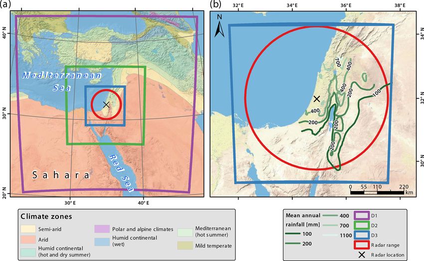
1228                                                   M. Armon et al.: Radar-based characterisation of heavy precipitation

networks and coarse-scale weather models (e.g. commonly             ing the atmospheric conditions that trigger HPEs or under-
used, global or even regional circulation models). Thus, high-      standing the overall rainfall pattern in comparison to obser-
resolution observation and HPE forecasts remain a challenge         vational records (e.g. Flaounas et al., 2019; Kendon et al.,
(Borga et al., 2011; Collier, 2007; Doswell et al., 1996).          2014; Khodayar et al., 2018). Commonly, climate change
   Rain gauge data can be used to quantify general charac-          studies based on high-resolution NWP models characterise
teristics of HPEs (such as rain intensity and depth on a point      the expected changes in precipitation, focusing on rainfall
scale), but their density is generally insufficient to adequately   intensity or frequency, or some derived index (e.g. Ban et al.,
represent the spatial gradients, particularly in the case of        2014; Hochman et al., 2018b; Schär et al., 2016; Westra et al.,
sparsely gauged regions, short-lived events, and arid climates      2014).
(Amponsah et al., 2018; Kidd et al., 2017; Morin et al., 2009,         A basic question, however, remains open: to what degree
2020). This problem is enhanced in regions characterised by         is the model description of rainfall during HPEs credible?
high climatic gradients such as the eastern Mediterranean,          Moreover, the model’s ability to reproduce rainfall patterns
hereafter referred to as “EM” (El-Samra et al., 2018; Marra         can differ among synoptic types. To answer this question,
et al., 2017; Marra and Morin, 2015; Morin et al., 2007;            both a realistic spatiotemporal representation of rainfall dur-
Rostkier-Edelstein et al., 2014). Thus, a high-resolution char-     ing HPEs and a large number of observed HPEs, triggered
acterisation of HPEs in such regions must be supported by           by various synoptic systems, are necessary. In this paper, we
other types of records. Remotely sensed precipitation es-           present a successful step in this direction based on a cor-
timates, such as those acquired from weather radars, pro-           rected and calibrated 24-year-long record of weather radar
vide the necessary spatiotemporal resolutions (e.g. 1 km and        data recently developed for the EM, which has been found
5 min) and coverage (regional scale) and have been shown            to adequately represent extreme precipitation events (Marra
to be useful for analysing specific events (e.g. Borga et al.,      and Morin, 2015). As an essential step in understanding and
2007; Dayan et al., 2001; Krichak et al., 2000; Smith et al.,       quantifying rainfall-generating processes involved in HPEs
2001). Where continuous radar records exist, they have been         and as a basis for a future study that will include downscaling
used in climatological studies as well (Belachsen et al., 2017;     of climate change projections to understand changes in rain-
Bližňák et al., 2018; Peleg and Morin, 2012; Saltikoff et al.,     fall patterns, here we aim to (i) characterise high-resolution
2019; Smith et al., 2012). However, climatological charac-          rainfall patterns (seasonality, spatial distribution of inten-
terisations of rainfall patterns during HPEs are rare in the lit-   sities, location, and spatiotemporal structure) during HPEs
erature and often based on rain gauge identification of those       in the hydroclimatically heterogeneous EM and (ii) assess
events (Panziera et al., 2018; Thorndahl et al., 2014).             the capabilities of a regional convection-permitting weather
   High-resolution numerical weather prediction (NWP)               model to simulate these patterns. To this aim, we identified
models allow for the simulation and forecasting of HPEs,            all HPEs embedded in the radar record (41 events) and simu-
and, as added value, they enable an understanding of their          lated them using a convection-permitting Weather Research
past and present patterns to be developed as well as a pre-         and Forecasting (WRF) model (Skamarock et al., 2008). This
diction of possible future behaviours (Cassola et al., 2015;        long and consistent high-resolution dataset is unique; thus, it
Deng et al., 2015; El-Samra et al., 2018; Kendon et al.,            is interesting both for examining HPE climatology and as a
2014; Prein et al., 2015; Rostkier-Edelstein et al., 2014; Yang     basis for convection-permitting model evaluation. Consider-
et al., 2014). In particular, convection-permitting models are      ing that our observations are based on radar data, they are
increasingly used in weather forecasts, climatological stud-        certainly not perfect. Therefore, we quantified and compared
ies, and event-based reanalyses (e.g. Ban et al., 2014; Fosser      several rainfall characteristics from both radar estimates and
et al., 2014; Hahmann et al., 2010; Khodayar et al., 2016;          simulated rainfall to evaluate the model’s ability to reproduce
Prein et al., 2015; Rostkier-Edelstein et al., 2015). Such mod-     the rainfall patterns and to obtain climatological characteris-
els downscale global or regional NWP models and provide             tics of HPEs.
a direct representation of convective rainfall that, due to its        The paper is structured as follows: Sect. 2 describes the
high intensity and local characteristics, often plays a ma-         study region; the radar and weather model data are explained
jor role in HPEs (e.g. Flaounas et al., 2018). In addition,         in Sect. 3.1 and 3.2, respectively; identification and synoptic
these models can provide 3-D fields of otherwise unmea-             classification of HPEs are presented in Sect. 3.3 and 3.4, re-
surable meteorological variables, thereby contributing to our       spectively; the methods used to evaluate model performance
understanding of the dynamics of HPEs. Studies based on             are presented in Sect. 3.5; Sect. 4 presents the results of
high-resolution NWP models commonly focus on specific               the evaluation and characterisation of rainfall patterns during
cases. For example, Zittis et al. (2017) examined the perfor-       HPEs; Sect. 5 provides a discussion; and Sect. 6 concludes.
mance of a high-resolution NWP model during five HPEs in
the EM and identified large discrepancies between grid- and
gauge-based precipitation datasets, making it hard to vali-
date the model. Only a few studies have examined the cli-
matology of model results, with the aim of either determin-

Hydrol. Earth Syst. Sci., 24, 1227–1249, 2020                                    www.hydrol-earth-syst-sci.net/24/1227/2020/
M. Armon et al.: Radar-based characterisation of heavy precipitation                                                        1229

2     Study region                                                 31.998◦ N, 34.908◦ E). Its effective range is 185 km. Raw
                                                                   radar reflectivity data were translated to quantitative pre-
This study focuses on the EM region, where Mediterranean           cipitation estimates (QPEs) using a fixed Z–R relationship
climate (which can reach a mean annual precipitation of            (Z = 316 · R 1.5 ) and applying physically based corrections
more than 1000 mm yr−1 ) drops to hyperarid (less than             and gauge-based adjustment procedures (see details in Marra
50 mm yr−1 ) over a short distance (Goldreich, 2012) (Fig. 1).     and Morin, 2015). This produced QPEs at 1 km2 and roughly
Precipitation is dominated by rainfall, and it mainly occurs       5 min resolutions. Examining the radar QPE and compar-
between October and May, with summer months (June to               ing it with rain gauges at an hourly and yearly resolution
September) being essentially dry (Kushnir et al., 2017). Most      yielded a root-mean-square error of 1.4–3.2 mm h−1 and 13–
of this rainfall is associated with cold north-westerly flows in   220 mm yr−1 , respectively, and a bias of 0.8–1.1 (hourly)
the rear part of Mediterranean cyclones (MCs). These MCs           and 0.9–1.1 (yearly) (Marra and Morin, 2015). This archive
pass above the warm water of the Mediterranean Sea, absorb-        has previously been used for a series of studies focusing
ing moisture and precipitating it over the EM region (Alpert       on high-intensity precipitation, including precipitation fre-
et al., 2004; Alpert and Shay-EL, 1994; Armon et al., 2019;        quency analysis (Marra et al., 2017; Marra and Morin, 2015),
Saaroni et al., 2010; Ziv et al., 2015). High surface water        floods (Rinat et al., 2018; Zoccatelli et al., 2019), and char-
temperature favours high-intensity rainfall and floods, most       acterisation of convective rain cells (Belachsen et al., 2017;
commonly at the beginning of the rainy season and near the         Peleg et al., 2018). A few of the following issues potentially
sea. As the MCs move inland and towards the desert, a sub-         affecting the QPE should be mentioned. The radar was turned
stantial amount of the moisture is lost, and rainfall occur-       off during the dry season and, for technical reasons, some-
rence and amounts are greatly reduced (Enzel et al., 2008).        times during the wet season; thus, a few severe storms were
In this arid region, HPEs are associated not only with MCs         missed and are not included in the archive. A long-term de-
(Kahana et al., 2002) but also with active Red Sea troughs         cline in the availability and quality of radar data might have
(ARSTs) (Ashbel, 1938; Krichak et al., 1997; De Vries et al.,      decreased the number of high-quality archived HPEs over
2013) and, more rarely, with tropical plumes (Armon et al.,        the years, mainly since 2010. As we did not aim to provide
2018; Rubin et al., 2007; Tubi et al., 2017). Commonly, rain-      a complete climatology, these aspects were not expected to
fall during ARSTs is of a spotty nature, can reach far into the    influence the results of the study. For technical reasons, the
desert, and can be of very high intensity (Armon et al., 2018;     radar products were not always available at their intended
Sharon, 1972). Conversely, during tropical plumes, rainfall        temporal resolution (approximately 5 min) and longer gaps
is widespread, potentially covering most of the region simul-      may exist between consecutive radar scans. Gaps of less than
taneously with moderate intensities. Desert HPEs frequently        20 min between consecutive radar scans were linearly inter-
result in large and sometimes devastating flash floods (e.g.       polated to recreate the 5 min resolution; gaps of more than
Armon et al., 2018; Dayan and Morin, 2006; Farhan and An-          20 min were treated as missing data. Due to the uneven spa-
bar, 2014; Kahana et al., 2002; Saaroni et al., 2014; Seager       tial distribution of the rain gauges, adjustment procedures
et al., 2014). Projections for precipitation in the EM indicate    may inadequately represent the south-easternmost areas cov-
a substantial decrease in annual rainfall amounts (Giorgi and      ered by the radar, where the gauge network is most sparse.
Lionello, 2008). However, the importance of credible HPE           Finally, due to overshooting of the radar beam, precipitation
simulations stems from, among others, opposing trends that         occurring east of the Dead Sea (Fig. 1) is generally underes-
may appear between the number and intensity of HPEs gen-           timated.
erated by different synoptic conditions (Alpert et al., 2002;
Hochman et al., 2018b, 2020; Marra et al., 2019); for exam-        3.2   WRF model configuration
ple, based on Dead Sea sedimentological data, it has been
suggested that when MC frequency is reduced, i.e. there is a       The WRF model was configured using three two-way nested
regional drought, the frequency of HPEs generated by AR-           domains, with a 1 : 5 resolution ratio between them (Fig. 1)
STs may increase (Ahlborn et al., 2018).                           and 68 vertical levels (model top is at 25 hPa). The inner
                                                                   domain (551 pixels× 551 pixels) was set at a 1 km2 hori-
                                                                   zontal resolution, in order to be comparable with the radar
3     Methodology and data                                         data. To comply with the Courant–Friedrichs–Lewy numer-
                                                                   ical stability criterion, model time steps in the innermost
3.1    Weather radar data                                          domain were between 4 and 8 s (Warner, 2011). However,
                                                                   to spare computer storage, outputs were saved at 10 min
The weather radar data used in this study consist of 24 hy-        intervals. When analysed, the WRF grid was interpolated
drological years (September–August), between 1990–1991             using nearest-neighbour interpolation from a Lambert pro-
and 2013–2014, observed by the Electrical Mechanical Ser-          jection grid to a similar-sized grid on a transverse Merca-
vices (EMS/Shacham) non-Doppler C-band weather radar               tor projection, as in the radar archive. It is important to
(5.35 cm wavelength), located at Ben Gurion Airport (Fig. 1;       note that a 1 km2 spatial resolution enables the explicit res-

www.hydrol-earth-syst-sci.net/24/1227/2020/                                     Hydrol. Earth Syst. Sci., 24, 1227–1249, 2020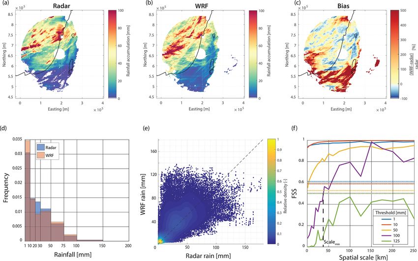
1230                                                     M. Armon et al.: Radar-based characterisation of heavy precipitation

Figure 1. Study region. (a) Climate zones in the eastern Mediterranean, three nested domains used in the weather model (D1-3; purple,
green, and blue) and the radar domain (red). (b) Mean annual rainfall isohyets, radar, and innermost model domains. Climatic classification
is from the Atlas of Israel (2011). Basemap source: U.S. National Park Service.

olution of convection, without the use of parameterisation              fined quantile (e.g. 95th or 99th) or a high but constant in-
(e.g. Prein et al., 2015). The two outer domains used the               tensity (e.g. 10, 20, or 50 mm d−1 ; see Drobinski et al., 2014;
WRF Tiedtke scheme for the parameterisation of convection               Nuissier et al., 2011; Westra et al., 2014; X. Zhang et al.,
(Tiedtke, 1989; C. Zhang et al., 2011). The model input data            2011). In contrast, hydrological definitions usually focus on
were 6-hourly ERA-Interim reanalyses, at approximately an               the resulting flood. In general, a good definition of a HPE
80 km horizontal resolution, and with 60 vertical levels, in-           should also include the areal dimension to enable hydrolog-
cluding sea surface temperature, along with basic meteoro-              ical and social impacts to be taken into account (Easterling
logical parameters (Dee et al., 2011). The model was used to            et al., 2000).
simulate the HPEs identified in the radar archive (Sect. 3.3;              Here we define HPEs by the exceedance of local, quantile-
Table S1 in the Supplement). Each simulation started 24 h               based thresholds over a sufficiently large area. The decision
prior to the beginning of the event, rounded down to the pre-           to set local thresholds was due to the sharp climatic gradi-
vious 6 h, and finished at the end of the HPE, rounded up to            ent characterising the study area. To decrease the computa-
the next 6 h. Therefore, the spin-up period of each simulation          tional effort and guarantee adequate temporal sampling, the
was at least 24 h. Additional model settings, presented in Ta-          HPE identification was based on a radar database compris-
ble 1, were selected because they are considered suitable for           ing hourly intervals for which at least 60 % of the expected
convection-permitting simulations (e.g. Romine et al., 2013;            radar scans were available (Marra et al., 2017). For a set of
Schwartz et al., 2015).                                                 durations between 1 and 72 h, we defined the threshold as
                                                                        the 99.5th quantile of the non-zero (i.e. more than 0.1 mm)
3.3    HPE identification                                               hourly amounts observed in each radar pixel. The range of
                                                                        examined durations was chosen to represent both short- and
HPEs have various definitions in different research fields and          long-lived HPEs. It should be noted that the same storm can
geographical regions. For example, climatologically, HPEs               be identified as a HPE for multiple durations. Depending on
are commonly associated with a specific time interval (i.e.             the duration and location, the amounts obtained are equiva-
sub-daily to a number of consecutive days) during which pre-            lent to annual return periods of roughly 2–10 years (Fig. 2).
cipitation depth surpasses a threshold representing a prede-            To account for the spatial scale, we classified all time inter-

Hydrol. Earth Syst. Sci., 24, 1227–1249, 2020                                          www.hydrol-earth-syst-sci.net/24/1227/2020/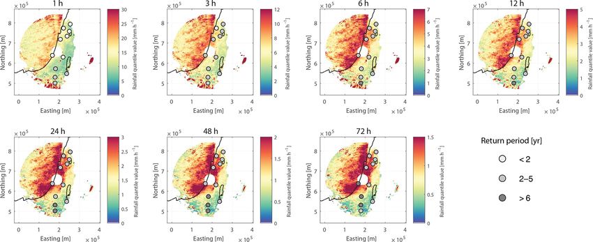
M. Armon et al.: Radar-based characterisation of heavy precipitation                                                                  1231

Table 1. WRF model settings and specifications.

                                                                 Outer nest    Middle nest    Inner nest
               Domains
               Spatial resolution (km)                           25 × 25       5×5            1×1
               Temporal resolution (s)                           ∼ 100         ∼ 20           4–8
               Domain size (pixels)                              100 × 100     221 × 221      551 × 551
               Number of vertical layers                         68            68             68
               Model top (hPa)                                   25            25             25
               Physics
               Cumulus scheme (outer and middle nests only)      Tiedtke (Tiedtke, 1989; C. Zhang et al., 2011)
               Microphysical scheme                              Thompson (Thompson et al., 2008)
               Radiative transfer scheme                         RRTMG short wave and long wave (Iacono et al., 2008)
               Planetary boundary layer scheme                   Mellor–Yamada–Janjić (Janjić, 1994)
               Surface layer scheme                              Eta similarity scheme (Janjić, 1994)
               Land surface model                                Unified Noah land surface (Tewari et al., 2004)

Figure 2. The 99.5 % rain intensity quantile of each radar pixel for durations of 1 h (top-left panel) to 72 h (bottom-right panel). Notice
the change in the colour scale between different durations. Also shown are annual return periods of the rain-intensity threshold averaged
over nine pixels around 11 locations (generalised extreme value fit of the rain gauge annual maxima series, using the method of probability-
weighted moments, with records of at least 44 years). These computed annual return periods range between 1.8 and 10.4 years. White areas
found mostly to the east of the radar were masked out according to the black line in Fig. 6c (Sect. 4.2).

vals during which at least 1000 pixels (i.e. 1000 km2 ) ex-             and Morin (2015), storms were separated by at least 24 h with
ceed their local threshold as HPEs. Jointly, these thresholds           less than 100 pixels displaying rainfall of more than 0.1 mm.
(99.5 % for each pixel, and an aggregation of 1000 pixels for           As the ERA-Interim data are available at a 6 h resolution,
an event) settle the trade-off between having too many (or              rainstorms that were too short (less than 12 h) were excluded
too few) events and accounting for HPEs that are too local              from the analysis. Storms longer than 144 h were excluded
(or only including the most widespread rainstorms). These               to avoid major changes in sea surface temperature during
selected thresholds enable the analysis of a reasonable num-            events. In addition, events were discarded manually when the
ber of diverse HPEs, with some being quite local and others             radar data were abundantly contaminated by ground clutter
more widespread.                                                        due to anomalous propagation or when other data-quality is-
   The selection procedure yielded 76–98 individual events              sues were observed. The final list of HPEs consisted of 41 in-
for each of the examined durations, summing to 120 when                 dependent events spanning 3.4±1.6 d on average (Table S1).
overlaps between durations were included. Similar to Marra

www.hydrol-earth-syst-sci.net/24/1227/2020/                                           Hydrol. Earth Syst. Sci., 24, 1227–1249, 2020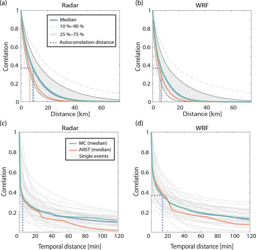
1232                                                    M. Armon et al.: Radar-based characterisation of heavy precipitation

   For each of these events, a filter was used to remove pix-        more suitable for high-resolution rainfall fields range from
els with residual ground clutter. Pixels in which the prob-          simple visual comparisons to more sophisticated, object-
ability of rain detection (POD, i.e. the fraction of time in         oriented or filtering methods capable of representing spa-
which the pixel exceeds 0.1 mm h−1 ) exceeds 10 % and is             tiotemporal properties of the fields (e.g. Davis et al., 2006;
larger than 1.9 times the average POD of the surrounding             Gilleland et al., 2009; Roberts and Lean, 2008). In this study,
area (25 km × 25 km) were removed. The extent of the ex-             we applied visual comparisons and several numerical mea-
plored area and of the ratio were chosen subjectively after          sures to compare the observed radar QPE with the WRF-
examining ranges between 1 and 3 (for the ratio) and 5 and           derived rain field.
50 km (for the areal extent). Additional areas known to be
persistently contaminated by ground echoes (from our expe-           3.5.1   Fractions skill score
rience and earlier studies) were masked out manually (e.g.
the circular area near the radar). Together, these procedures        To evaluate rainfall accumulation for different neighbour-
excluded approximately 0.5 % of the radar pixels.                    hood sizes (namely, spatial scales), we used the method sug-
                                                                     gested by Roberts and Lean (2008). The methodology in-
3.4    Synoptic classification                                       cludes a conversion of the continuous rain field to a binary
                                                                     field based on the exceedance of a given rain-depth thresh-
We classified the HPEs into two classes representing the             old. The fraction of model-output positive pixels (i.e. pixels
most common rainy synoptic circulation patterns prevailing           that have exceeded the threshold) within a certain neighbour-
in the region: MC and ARST. To do so, we relied on the               hood size is then compared with the matching fraction from
semi-objective synoptic classification by Alpert et al. (2004),      the radar QPE, via the fractions skill score (FSS) statistic
based on daily (at 12:00 UTC) meteorological fields at the           (Sect. S1 in the Supplement). When the forecast is perfect
1000 hPa pressure level from the NCEP/NCAR reanalysis                and unbiased, i.e. when an equal number of observed (in our
(2.5◦ spatial resolution). We classified a HPE as a MC if one        case, radar) and forecasted (WRF) pixels exceed the thresh-
of the following conditions occurred: (i) most of the days           old, the FSS is equal to 1. If there is a bias, the FSS will tend
comprising the HPE were considered, according to Alpert              asymptotically to a lower value. To quantitatively evaluate
et al. (2004), as days with either a MC or a high-pressure           the model’s ability to predict the observed rainfall above the
system following a MC; (ii) one of the days during the HPE           selected threshold, within a close-enough distance, the uni-
was a MC and none of them were an ARST. Similarly, we                form FSS (halfway between a random forecast and a perfect
classified a HPE as an ARST if (i) most of its days were clas-       skill forecast, yielding a hit rate of 0.5; Sect. S1) is also calcu-
sified as ARST according to Alpert et al. (2004) or (ii) one         lated. A FSS that is larger than the uniform FSS is considered
of its days was an ARST and none of them were a MC.                  skilful. It is important to note that if the FSS exceeds the uni-
The above-mentioned tropical plume synoptic pattern (Rubin           form FSS on too large a spatial scale, the forecast might still
et al., 2007; Tubi et al., 2017) is not part of our classification   be skilful, but it is not useful. We applied the FSS method
because of its low frequency and because it does not appear          to the cumulative rain field, comparing the radar QPEs and
in near-sea-level pressure meteorological fields. Specifically,      WRF rainfall output (Sect. 4.3).
one HPE (HPE 41; Table S1) was characterised, during its 5 d
span, first by the prevalence of a tropical plume (Armon et al.,     3.5.2   Structure–amplitude–location analysis
2018) and then by a MC; it was classified here as a MC. De-
spite the simplification, these two classes have recently been       To evaluate the characteristics of the WRF precipitation fore-
shown to exhibit distinct characteristics of rainfall intensity      cast errors, we used the object-oriented structure–amplitude–
distribution (Marra et al., 2019). Indeed, 85 % and 15 % of          location (SAL) analysis (Wernli et al., 2008) (Sect. S2 in the
HPEs were classified as MCs and ARSTs, respectively (Ta-             Supplement). As in the FSS analysis, it was applied to the cu-
ble S1), reasonably following the expected proportions of the        mulative rain field. The SAL analysis splits the rain field into
two synoptic circulation patterns (Goldreich et al., 2004; Saa-      three distinct components and yields a skill score for the fore-
roni et al., 2010).                                                  cast of each of them; in each of the components, a zero score
                                                                     indicates a perfect forecast. The amplitude component (A)
3.5    Evaluation of simulated rain fields                           expresses the model’s over- or underestimation of the total
                                                                     rainfall for a specific rainstorm (with A ∈ [−2, 2], and A = 1
Inaccurate initial conditions in the presence of non-linear          or A = −1 indicating over- and underestimation by a fac-
precipitation-generation processes, along with the presence          tor of 3, respectively). The location component (L ∈ [0, 2])
of atmospheric instabilities, may limit the atmospheric pre-         sums the differences between modelled and observed (i) cen-
dictability and, consequently, modelling skill (Anthes et al.,       tre of mass of precipitation and (ii) average distance between
1985). Moreover, increasing the model resolution may pose            the centre of mass and the location of precipitation objects
difficulties in a pixel-by-pixel evaluation of the forecasts (e.g.   that constitute the rain field (i.e. connected regions in which
Davis et al., 2006; Mass et al., 2002). Approaches that are          the cumulative rainfall exceeds 1/15 of the maximal cumu-

Hydrol. Earth Syst. Sci., 24, 1227–1249, 2020                                       www.hydrol-earth-syst-sci.net/24/1227/2020/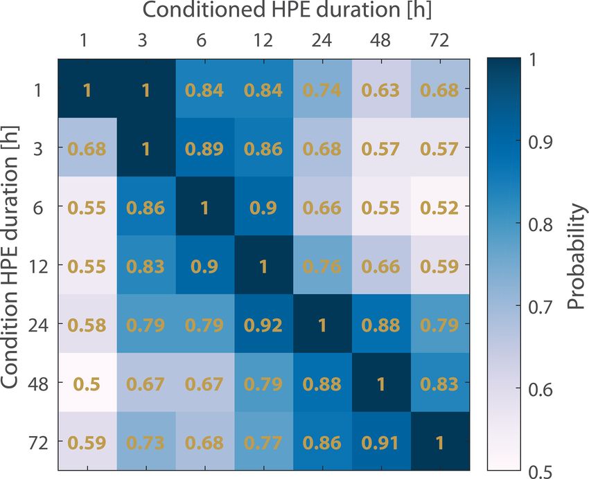
M. Armon et al.: Radar-based characterisation of heavy precipitation                                                            1233

lated value; Wernli et al., 2008). The structure component
(S ∈ [−2, 2]) quantifies the tendency of the forecasted pre-
cipitation objects to be either too smooth (positive values) or
too noisy (negative values) relative to the observations.

3.5.3   Depth–area–duration curves

Areal rainfall amounts are crucial drivers of the hydrolog-
ical response and are important for understanding rainfall
structure and triggering mechanisms (e.g. Armon et al., 2018;
Durrans et al., 2002; Kalma and Franks, 2003; Zepeda-Arce
et al., 2000). To quantify and compare observed and sim-
ulated areal rainfall amounts, we used depth–area–duration
                                                                   Figure 3. Monthly probability of occurrence of rainy days near the
(DAD) curves, which represent the areal extent for which
                                                                   radar location (green; Bet Dagan rain gauge; 32.0◦ N, 34.8◦ E), and
given rainfall depths over specific durations are exceeded
                                                                   of HPEs from the radar archive (orange). Hatching represents HPEs
(Zepeda-Arce et al., 2000).                                        classified as ARSTs.

3.5.4   Autocorrelation structure of rain fields
                                                                      The temporal autocorrelation is computed by converting
High-intensity, small-scale convective rain cells are among
                                                                   the 2-D spatial domain to a 1-D array and adopting time
the main factors generating flash floods in small, mountain-
                                                                   as the second dimension, as proposed by Marra and Morin
ous and desert catchments (e.g. Armon et al., 2018; Doswell
                                                                   (2018). It is worth noting that the computed temporal corre-
et al., 1996; Merz and Blöschl, 2003), and their fine spa-
                                                                   lation distance neglects advection (Eulerian perspective) and
tiotemporal structure directly affects the potential of rain
                                                                   is therefore shorter than the correlation distance obtained in
gauge monitoring (Marra and Morin, 2018). To analyse the
                                                                   a Lagrangian perspective.
convective rain structure, we computed the spatial autocorre-
lation structure of the maps containing convective elements
from both the observed radar QPE and the WRF output using
                                                                   4     Results
the methodology presented by Marra and Morin (2018) (an
example is given in Fig. S1). We interpolated the radar QPEs
                                                                   4.1    Quasi-climatology of HPEs
to 10 min intervals to match the model’s temporal resolution,
and defined all rain maps in which at least one convective rain
                                                                   Of the 41 identified HPEs, 35 occurred during MC synoptic
cell (defined as a connected region ≥ 3 km2 with rain inten-
                                                                   prevalence and the rest during ARST prevalence. Despite the
sity exceeding 10 mm h−1 and including at least one pixel ex-
                                                                   dependence of the identification on the quality and availabil-
ceeding 25 mm h−1 ) is observed as convective rainfall fields
                                                                   ity of the radar data, our analysis can be considered “quasi-
(Marra and Morin, 2018). We computed the 2-D spatial au-
                                                                   climatological”, as the selected HPEs do not exhibit obvi-
tocorrelation function of the convective fields following the
                                                                   ous biases with respect to the rain climatology in the region:
method in Nerini et al. (2017). A three-parameter exponential
                                                                   (i) their seasonality follows the seasonal pattern of EM rainy
function (Eq. 1) was fitted to the 2-D spatial autocorrelation
                                                                   days (Fig. 3), although HPEs occur more frequently at the
to quantify the correlation distance:
                                                                   beginning of the winter, presumably due to the high sea sur-
                 c
                 h
                                                                   face temperatures; (ii) HPEs are identified throughout the
            −    b
r(h) = ae              ,                                    (1)    radar archive (with zero to seven HPEs per year); (iii) the
                                                                   frequency of the prevailing synoptic circulation patterns dur-
where h is the lag distance, b is the correlation distance (the    ing HPEs (Table S1) resembles the frequency observed on
distance at which the correlation drops to r = e−1 ), and a        rainy days (Marra et al., 2019); and (iv) HPEs characterised
and c are the nugget and shape parameters of the curve, re-        by ARST prevalence are common only during the transition
spectively. Equation (1) results in an approximation of the        seasons (Fig. 3 in this paper; e.g. De Vries et al., 2013).
1-D autocorrelation function of convective rain fields. The           For most examined durations, rain amounts defining the
spatial heterogeneity of the autocorrelation field is quantified   HPEs are larger near the Mediterranean coast, extending a
by calculating the deviation of the 2-D autocorrelation field      few kilometres off- and onshore (Fig. 2). This resembles
from isotropy, following the approach in Marra and Morin           the observed pattern of high rain intensities near the coast,
(2018). To this end, we defined the ellipticity of the 2-D au-     rather than inland (Karklinsky and Morin, 2006; Peleg and
tocorrelation as the ratio of the minor to major axis of the       Morin, 2012; Sharon and Kutiel, 1986), which has also been
(approximated) ellipse encompassing the r = e−1 region of          reported for extreme precipitation quantiles observed from
the spatial autocorrelation field (Fig. S1).                       both weather radar and satellite sensors (Marra et al., 2017).

www.hydrol-earth-syst-sci.net/24/1227/2020/                                        Hydrol. Earth Syst. Sci., 24, 1227–1249, 2020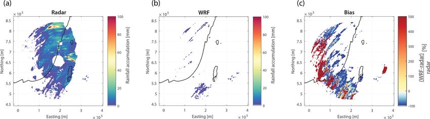
1234                                                   M. Armon et al.: Radar-based characterisation of heavy precipitation

In contrast, short durations (less than 12 h) exhibit the highest   4.2   Bias
rain intensities in the arid areas of the region. The frequency
of rain in the arid areas is lower than in the rest of the re-      Figure 6 shows the rainfall accumulated during all HPEs as
gion (Goldreich, 2012); thus, the 99.5 % quantiles are based        estimated by the weather radar, modelled by the WRF, and
on fewer data. Nevertheless, the reported higher extreme rain       measured by rain gauges (Fig. 6a, b, and d, respectively).
amounts for shorter durations are in agreement with previ-          Bias, defined herein as the normalised
                                                                                                                difference
                                                                                                                            between
ous studies, which showed that highly localised convective                                              WRF−radar
                                                                    WRF rainfall and radar QPE             radar      , in percent, is
rainfall is more common during HPEs in the desert than in           shown in Fig. 6c. In 69 % of the studied region, the bias lies
other climatic environments in the EM (Marra et al., 2017;          between +200 % and −67 %, although some areas show a
Marra and Morin, 2015; Sharon, 1972). In the mountains,             strong positive bias (Fig. 6c). The three stations highlighted
the opposite case is seen: rainfall is produced more signifi-       in the figure (the values shown for radar and WRF represent
cantly through stratiform (or shallow convection) processes,        the average of the nine pixels surrounding the gauge loca-
and rain amounts for short durations are therefore relatively       tions) show how this large bias is mostly caused by radar
lower (Sharon and Kutiel, 1986). For the longer durations,          underestimation. In fact, these areas are generally located far
rain intensities in the mountains are comparable to the in-         from the radar or in the eastern portion of the radar coverage,
tensities near the coast, probably resulting from the tendency      where radar QPE suffers from range degradation and beam
of rain to persist in orography-affected regions (e.g. Panziera     overshoot due to the presence of mountains. In some other
et al., 2015; Tarolli et al., 2012).                                areas, the bias seems related to residual beam blockages. Un-
   Affected by higher rain intensities, the centre of mass of       derestimation (a bias less than zero) is also apparent in re-
the precipitation field for each of the HPEs is located near the    gions with ground clutter, and some spatial inconsistencies
EM coastline (Fig. 4). Nevertheless, a seasonal pattern ap-         related to the interpolation of a few fully blocked beams can
pears, with a general landward shift of the centre of mass dur-     also be noticed. To avoid interference of these radar estima-
ing the rainy season (Fig. 4). This is caused by land–sea dif-      tion inaccuracies with our results, we focus only on the areas
ferential heating and heat capacities and resembles the sea-        in which the bias lies between +200 % and −67 % (Fig. 6c).
sonal pattern of rain intensities in the EM (Goldreich, 1994;       Still, a portion of the area close to the radar is characterised
Sharon and Kutiel, 1986). In fact, this points out the ob-          by negative bias, which could be attributed to simulated rain
served preference of convective clouds to form above high-          intensities that are too low. A similar pattern was also shown
temperature surfaces, i.e. the sea surface or nearby coastal        in Rostkier-Edelstein et al. (2014) where it was attributed to
plains in autumn or early winter as well as farther inland in       intensities that were too low during deep MCs.
the spring. In terms of seasonality, the WRF-simulated cen-
tres of mass exhibit a similar, even if slightly less obvious,      4.3   Visual, neighbourhood and object-based evaluation
landward pattern. It must be noted that ARST-type events                  of WRF model simulations
in the WRF results are biased eastwards compared with the
radar results, which could be related to the WRF’s worse per-       Visual comparison of observed (radar) and simulated (WRF)
formance with respect to such events (e.g. Sect. 4.3). More-        rainfall fields yielded mostly (subjectively) good results in
over, the exact location of the radar-observed centre of mass       terms of the spatial rainfall patterns, such as widespread ver-
can suffer from range degradation, which may cause these            sus localised rainfall. As an example, Fig. 7 presents a well-
centres to be biased towards the radar location.                    simulated HPE case (HPE 1, Table S1). In addition, the dis-
   According to the definition applied in this study, a given       tributions of rainfall among pixels were generally well repre-
event can be considered a HPE for more than one dura-               sented (Fig. 7d). At the same time, pixel-based comparisons
tion. This can happen when the thresholds associated with           were deemed inappropriate for such an analysis, as shown
the examined durations (Sect. 3.3) are exceeded either at the       in the scatter plot (Fig. 7e). Most of the examined HPEs led
same location or in different regions. The durations associ-        to similar observations, with the exception of two HPEs in
ated with each HPE are listed in Table S1. The co-occurrence        which the WRF model clearly failed to represent the rain-
of each HPE duration with the rest of the examined durations        fall patterns. An example of such a poor simulation is given
is shown in Fig. 5; these co-occurrence values are similar to       in Fig. 8 (HPE 5, Table S1). Both of these poorly simu-
values determined in the Alps by Panziera et al. (2018). For        lated HPEs were characterised by relatively short total storm
example, 79 % of the HPEs at a 24 h duration are also HPEs          spans (1.7 and 2 d), just exceeding the durations that defined
at a 72 h duration. Figure 5 indicates a high dependence (i.e.      them as HPEs (6 and 3–24 h, respectively). Synoptically, they
co-occurrence) of the short-duration HPEs (3–12 h). Simi-           were classified as ARSTs, a system generally characterised
larly, there is a high dependence within the long-duration          by local, short-lived convection associated with a localised
HPEs (24–72 h). Nevertheless, even the shortest (duration)          rainfall-triggering mechanism (Armon et al., 2018). The skill
HPEs examined here show a rather high co-occurrence with            of mesoscale models (e.g. WRF) is poorer in simulating these
the longest (duration) HPEs (probabilities in all cases greater     types of events, mainly due to their short predictability and
than or equal to 0.5).                                              stochastic nature (see e.g. Yano et al., 2018). Although a

Hydrol. Earth Syst. Sci., 24, 1227–1249, 2020                                     www.hydrol-earth-syst-sci.net/24/1227/2020/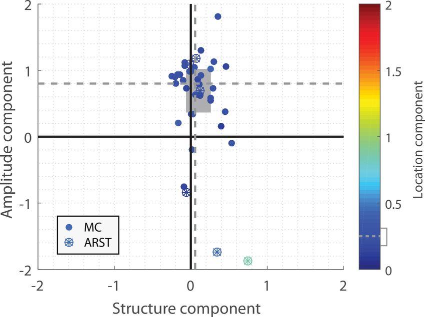
M. Armon et al.: Radar-based characterisation of heavy precipitation                                                            1235

Figure 4. Centres of mass of cumulative rainfall of each of the HPEs derived from (a) the radar QPE and (b) WRF. Colours represent the
month of occurrence. Synoptic classification according to Sect. 3.4.

                                                                     HPE, that the model forecast is unskilled at all spatial scales,
                                                                     i.e. the uniform FSS outperforms the WRF forecast FSS (yet,
                                                                     these results are also based on a limited number of data).
                                                                        During EM rainstorms, cumulative rainfall values are dis-
                                                                     tributed unevenly in space, and extremely high rainfall depths
                                                                     are embedded within the larger aerial coverage of lower rain-
                                                                     fall depths (e.g. Armon et al., 2018; Dayan and Morin, 2006;
                                                                     Morin et al., 2007). Thus, forecasting the spatial distribution
                                                                     (location and spatial frequency) of low cumulative rainfall
                                                                     is easier than forecasting the distribution of the high end of
                                                                     cumulative rainfall, even when averaging is conducted over
                                                                     large scales. The minimal scale (Roberts and Lean, 2008) at
                                                                     which the FSS of the model’s forecast is higher than the uni-
                                                                     form FSS was calculated for the occurrence of a range (1–
                                                                     200 mm) of cumulative rainfall depths for all of the identi-
Figure 5. Probability of a HPE with a given examined duration
listed on the x axis conditioned on being a HPE with a duration
                                                                     fied HPEs (Fig. 9). This allows for the estimation of the min-
listed on the y axis.                                                imal scales for skilful rainfall detection for rain depths that
                                                                     are equal to or greater than an arbitrary cumulative rain depth
                                                                     threshold. For example, the original model resolution yielded
                                                                     a skilful forecast for the occurrence of cumulative rainfall
deeper understanding of these aspects can be beneficial for          depths of less than 25 mm in 50 % of the HPEs (Fig. 9). The
improving future simulations, it falls outside the scope of this     figure also shows that the occurrence of cumulative rainfall
study and requires future dedicated research efforts.                exceeding 45 mm, in most cases, is only skilfully forecasted
   The FSS of the first HPE (Fig. 7f) further manifests the          on a relatively large spatial scale (tens of kilometres). Dur-
accuracy of the simulated rainfall fields. The forecast has a        ing ARSTs, the minimal scale was much higher than during
larger FSS than the uniform FSS for all of the examined cu-          MCs (not shown); however, it is important to remember that
mulative rainfall amounts less than or equal to 50 mm, even          two of these HPEs were poorly simulated.
at the model resolution (1 km). For larger cumulative rainfall,         The SAL analysis (Fig. 10) showed good performance of
the FSS is unstable due to the limited number of observations        the model, except for a substantial positive amplitude bias
of such cases; thus, no conclusions about the suitability of the     (inter-event amplitude component median of 0.80, i.e. a bias
results can be made for the occurrence of such high cumula-          of 130 %, as defined in Sect. 4.2, and interquartile range
tive rainfall. It is only for the higher rainfall amounts, e.g.      of 0.37–1.02). Two events stood out with a bias smaller
125 mm, corresponding to less than 1 % of the pixels in this         than zero; these were the above-mentioned poorly simulated

www.hydrol-earth-syst-sci.net/24/1227/2020/                                        Hydrol. Earth Syst. Sci., 24, 1227–1249, 2020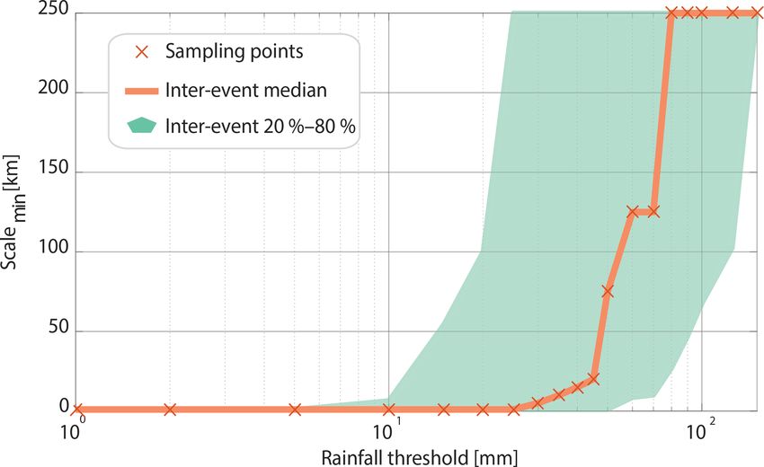
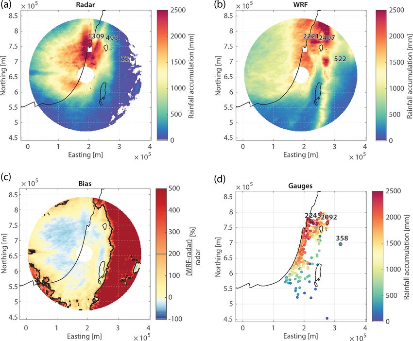
1236                                                    M. Armon et al.: Radar-based characterisation of heavy precipitation

Figure 6. Total cumulative rainfall for all 41 HPEs from (a) radar-derived QPE, (b) WRF-derived rainfall, and (d) daily rain gauges.
(c) WRF-to-radar rainfall accumulation bias (normalised difference; Sect. 4.2). The 200 % and −67 % bias region is marked in black. Total
accumulations (mm) measured at three rain gauges from regions where radar QPE is considered to be inferior are highlighted in panel (d);
corresponding radar and WRF nine-pixel averaged values (mm) centred over the same locations are shown in panels (a) and (b), respectively.

HPEs. In general, MC-type HPEs exhibited much greater                  or when intense rainfall is embedded within larger-scale low-
bias than ARSTs (inter-event amplitude component median                intensity precipitation (Wernli et al., 2009). The slight posi-
of 0.85 versus −0.07). However, it must be noted that the me-          tive tendency of the structure component could either indi-
dian of ARST-type HPEs includes the two poor simulations               cate that the model creates rain fields that are too smooth
and is therefore predicted to be more negative. Surprisingly,          (lower intensity rain and objects that are too large), that radar
where visual comparisons seemed better, and the structure              data are too noisy, or, most probably, a combination of both
component was closer to zero, the amplitude component ac-              error sources.
tually suffered from more positive biases; for example, the               Relatively low values of the location component (0.25 and
structure component of HPE 1 (Fig. 7, Table S1) is 0.04,               0.18 to 0.31 for the median and interquartile range, respec-
while its amplitude component is 1.03. Furthermore, the me-            tively; 0.26 and 0.22 are the medians for MC- and ARST-type
dian amplitude of events characterised by a structure compo-           events, respectively) demonstrate the model’s high capability
nent larger than the median structure is 27 % higher than the          to spatially distribute precipitation objects. Medially, 34 %
amplitude of events with a structure smaller than the median           of this component is composed of the error in the centre of
value.                                                                 mass location (namely L1 ; i.e. a median error of 30 km in
   The structure component was well modelled in most cases,            the location of the centre of mass), and the rest is from the
showing the ability of the WRF to accurately generate pre-             average location of each precipitation object (L2 ). Namely,
cipitation objects (0.06 and −0.06 to +0.26 for the median             the model prediction of the centre of mass of the rain field
and interquartile range, respectively; 0.05 and 0.09 are the           is quite satisfying, but the prediction of individual precipi-
medians for MC- and ARST-type events, respectively). This              tation objects is a bit poorer. The contribution from the L2
is particularly important in regions and for events where rain-        component to the location component (Sect. S2 in the Sup-
fall is generated via both convective and stratiform processes,        plement) indicates that modelled precipitation objects are not

Hydrol. Earth Syst. Sci., 24, 1227–1249, 2020                                         www.hydrol-earth-syst-sci.net/24/1227/2020/
M. Armon et al.: Radar-based characterisation of heavy precipitation                                                                          1237

Figure 7. HPE 1 (09:00 LT, 2 November 1991 to 09:00 LT, 5 November 1991; all times in the figure are given in local winter time; see
Table S1). Cumulative rainfall from (a) radar-derived QPE, (b) WRF-derived rainfall, and their ratio (c). A pixel-based comparison between
rainfall accumulations using a histogram (d; zero rainfall is omitted) and scatter plot (e). Notice that although the rainfall distribution is quite
well represented (d), results of a single pixel might deviate substantially from the 1 : 1 line (e; dashed). The fractions skill score (FSS) for the
same event for various cumulative rainfall thresholds is presented in panel (f). Dashed lines are uniform FSSs for the same rainfall thresholds.
The minimal scale for a valuable prediction for a 100 mm rain depth (at the crossing of the FSS and the uniform FSS; see Sect. S1 in the
Supplement for details) is also shown (dashed black line).

Figure 8. Same as Fig. 7a–c but for HPE 5 (09:00 LT, 31 March 1993 to 02:00 LT, 2 April 1993; Table S1).

distributed the same as the observed ones. This is probably                 values are rather small, exhibiting good spatial distribution of
due to a mismatch in the positioning of the simulated cells.                precipitation objects. Nonetheless, the same two challenging
Given the good ability of the radar to represent the location of            ARST-type HPEs for which the model was unable to simu-
rain cells, attenuation and range-degradation of the radar data             late the rainfall in a satisfying manner stand out with high
should only have minor effects on L2 . In either case, location

www.hydrol-earth-syst-sci.net/24/1227/2020/                                                Hydrol. Earth Syst. Sci., 24, 1227–1249, 2020
1238 M. Armon et al.: Radar-based characterisation of heavy precipitation
represent actual processes and rainfall characteristics (Wernli
et al., 2009).
4.4 Characterisation of rainfall patterns
4.4.1 Areal rainfall
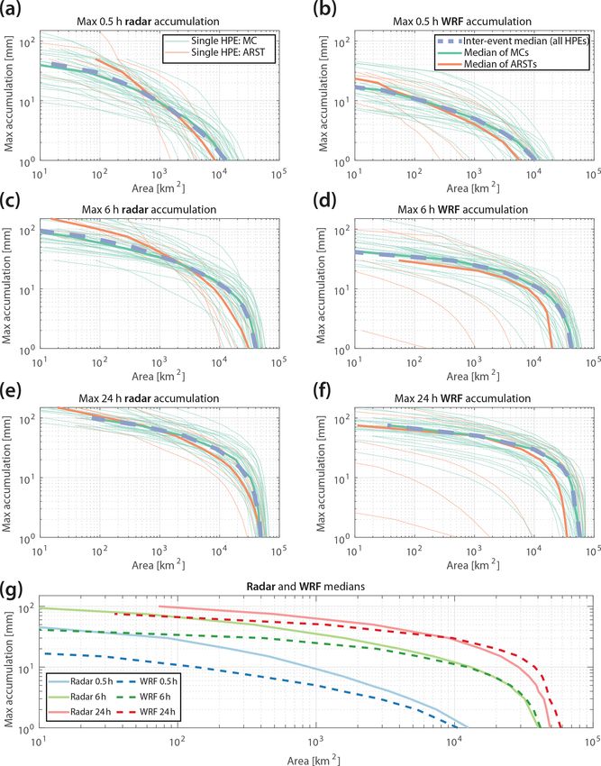
Figure 11 shows the depth–area–duration (DAD) curves ob-
tained from all 41 HPEs for durations of 30 min, 6 h, and 24 h
from radar QPEs (Fig. 11a, c, and e, respectively) and WRF
(Fig. 11b, d, and f, respectively). When referring to DAD
analysis, the term “duration” represents the time period, over
the course of each HPE, where maximum rainfall depths
Figure 9. Minimal scale (see Fig. 7f and Sect. S1 in the Supple- were observed. A major increase in cumulative rainfall with
ment) derived for all 41 events for various rainfall thresholds. increased duration is observed for both the radar and WRF
curves (Fig. 11g): for example, based on the radar, an area of
103 km2 is medially covered by 9 mm for a duration of 0.5 h,
which increases to 35 and 60 mm for 6 and 24 h, respectively
(corresponding values from the WRF-derived rainfall are 4,
25, and 50 mm). This increase could be explained by either
continuous rainfall or the frequent arrival of rain cells into
the region. The latter increases the wet area and the cumu-
lative rainfall in areas that have already experienced rainfall
and is a major characteristic of HPEs in the EM (e.g. Armon
et al., 2018, 2019; Sharon, 1972). Furthermore, over longer
durations, this causes DAD curves for different events to be
more similar to one another (e.g. Fig. 11e, f).
The inter-event spread and the difference in the DAD
curves for MC and ARST (Fig. 11a–f) illustrate the various
types of HPEs identified here. These types range between
rainstorms exhibiting only a minimal increase in rainfall area
Figure 10. Structure–amplitude–location (SAL) analysis (Wernli with time, i.e. almost all of the rainfall precipitates during a
et al., 2008). Each dot represents one event (classified according
short period; rainstorms composed of many rain cells passing
to Sect. 3.4). Dashed lines are median component values, and the
grey rectangle represents the 25th–75th percentile range. The loca-
through the same area; or long-lasting rainstorms. These re-
tion component median value is 0.25, and its 25th–75th range is sults confirm previous findings by Armon et al. (2018) based
0.18–0.31. More details are given in Sect. S2 in the Supplement. on a more limited number of events: HPEs classified as AR-
STs (Table S1) tend to have higher rain intensities for smaller
regions and shorter periods than HPEs classified as MCs.
MCs only exhibit higher rain intensities over larger regions
location values (0.46 and 0.85), yielding large spatial incon- and for longer durations.
sistency with respect to observations (see above, e.g. Fig. 8). It is important to note the difference between radar QPE-
The overall positive bias seen in the amplitude compo- and WRF-derived rainfall DAD curves. Higher rain values
nent (Fig. 10) could result from an underestimation of the in the radar QPE over the range of smaller areas is the most
radar QPE or an overestimation of the WRF simulation. Pos- obvious difference (Fig. 11g). Although these higher values
sible reasons leading to radar underestimation have been dis- may, at first glance, indicate that the WRF is unable to re-
cussed above and may contribute to this bias even after the produce the high-intensity rainfall of the HPEs in the EM,
most severely biased regions have been masked. However, it should be remembered that high-intensity radar QPEs can
this positive bias still needs to be considered when address- be of lower accuracy due to contamination from residual
ing the actual cumulative rainfall amounts predicted by the ground clutter or hail for short durations. This may affect
model. In contrast with the overall bias (Sect. 4.2) almost no the QPEs of the smaller areas more selectively. For instance,
event showed a negative bias. Rostkier-Edelstein et al. (2014) for one of the HPEs, an area of more than 100 km2 received
mainly attributed positive biases to deep lows over complex- a rain amount of greater than or equal to 100 mm in 0.5 h
terrain regions. (Fig. 11a) – a value that exceeds the 200-year return period
The overall good representation of precipitation objects for the area (Morin et al., 2009). Other notable differences are
implies that precipitation processes generated by the model some ARST-classified HPEs with WRF-derived DAD curves
Hydrol. Earth Syst. Sci., 24, 1227–1249, 2020 www.hydrol-earth-syst-sci.net/24/1227/2020/M. Armon et al.: Radar-based characterisation of heavy precipitation 1239
Figure 11. Depth–area–duration (DAD) curves showing the maximal amount of rainfall as a function of area, derived from the radar
QPE (a, c, e) and from the WRF model (b, d, f) for 0.5 h (a, b), 6 h (c, d), and 24 h (e, f). Green and orange lines represent HPEs clas-
sified as MCs and ARSTs, respectively. Thick lines represent the inter-event median. This median is compared between radar-QPE and WRF
rainfall in panel (g).
(Fig. 11b, d, f) consisting of the two WRF-unresolved HPEs 4.4.2 Autocorrelation structure of convective rainfall
mentioned above, and yielding a median ARST curve that is
much lower than the radar-derived curve. HPEs in the EM are commonly composed of highly localised
The reported differences between WRF- and radar-derived convective rain cells. This is well reflected in the sharp de-
curves result in an overall greater area-over-threshold radar crease of the 1-D autocorrelation describing the convective
curves for the high-rainfall thresholds, especially for the rain fields (Fig. 12a, b) obtained using all of the convective
short durations. For long durations and low rainfall thresh- rain fields throughout the 41 HPEs (n = 11 731 snapshots
olds, the WRF area is larger (Fig. 11), reflecting the positive for radar and n = 14 323 for WRF). The median decorrela-
bias mentioned above. tion distance (defined as the distance in which the correlation
drops to r = e−1 , i.e. parameter b of the 1-D exponential fit,
Eq. 1) of all convective rain snapshots from the radar data
is 9 km (7 km using the WRF-derived rainfall) and ranges
www.hydrol-earth-syst-sci.net/24/1227/2020/ Hydrol. Earth Syst. Sci., 24, 1227–1249, 20201240 M. Armon et al.: Radar-based characterisation of heavy precipitation
rainfall is expected, because radar QPE suffers from temporal
inconsistencies (e.g. when a convective cell passes through
a region with beam blockages). Nevertheless, such a short
temporal decorrelation confirms the local and spotty nature
of rainfall characterising HPEs in the region.
The declining pattern of the 1-D autocorrelation overlooks
the 2-D spatial heterogeneity of the autocorrelation field.
The ellipticity of the 2-D autocorrelation yielded a median
across all convective rain fields value of 0.56 (0.62 and 0.54
in ARST- and MC-type events, respectively), with a range
of 0.33–0.80 (10 %–90 % quantiles). WRF-derived ellipticity
values were almost the same: 0.58 (0.68 and 0.68 in ARST-
and MC-type events, respectively), with a range of 0.33–
0.79. These autocorrelation ellipses in the radar data were
oriented 13◦ anticlockwise from the east–west axis (median
value; 7 and 14◦ for ARST- and MC-types, respectively) and
22◦ for the WRF ellipses (10 and 24◦ for ARST- and MC-
types, respectively). These values are similar to the orien-
tation of radar rain cells in the eastern part of the region
(Belachsen et al., 2017), but they are somewhat different
from the orientation of autocorrelation fields from the south-
Figure 12. A 1-D exponential fitting of the rain field spatial (a, b) eastern part of the region (Marra and Morin, 2018). Orienta-
and temporal (c, d) autocorrelation values from radar-derived
tions found in the present analysis cover the entire evolution
QPE (a, c) and from the WRF model (b, d). These were computed
using 10 min snapshots of rain and only for periods where convec-
of HPEs and, thus, include both south-west (mainly at the
tive rainfall is present. Quantiles in spatial autocorrelation (a, b) beginning of the storm) and north-west (mainly at the end
represent 11 731 snapshots of radar 10 min data (10 095 of which of the storm) alignments of rain cells. Therefore, they are
come from MC-type events) and 14 323 WRF rainfall snapshots oriented more anticlockwise than the autocorrelation fields
(12 220 of which come from MC-type events). Temporal autocor- from the south-eastern part of the region (Marra and Morin,
relation plots (c, d) are composed of the 41 examined HPEs (grey) 2018), which commonly represents rainfall at the end of a
as well as their median values for all events (purple), for MC-type rainstorm (Armon et al., 2019). Moreover, Marra and Morin
only (green) and for ARST-type only (orange). (2018) examined 1 min snapshots, whereas here advection
can play a role in the examined 10 min time interval. Finally,
Marra and Morin (2018) only analysed 11 events; thus, inter-
between 3 and 23 km (for the 10 % and 90 % quantiles, re- event variance may still play a large role in their results. The
spectively; 2 and 20 km using WRF). The median decorrela- high agreement between modelled and observed rain field el-
tion distance during ARSTs is shorter than during MCs, as lipticity and orientation also demonstrates the high skill of
obtained from both the radar (7 and 10 km, respectively for the WRF simulations in accurately representing convection
ARSTs and MCs) and the WRF (5 and 7 km, respectively). in the region and, thus, reproducing rain cell properties.
These values are comparable to previously reported obser-
vations (e.g. Ciach and Krajewski, 2006; Morin et al., 2003; 4.5 Summary of results
Peleg and Morin, 2012; Villarini et al., 2008) and are some-
what larger than the reported values for the south-eastern part This work characterises rainfall patterns during 41 HPEs in
of the area by Marra and Morin (2018). However, it should be the EM and evaluates the ability of a high-resolution WRF
noted that Marra and Morin (2018) examined 1 min rainfall model to properly simulate their cumulative rain field and
fields versus the 10 min fields examined here. spatiotemporal behaviour, with a specific emphasis on their
The median of the temporal decorrelation distance convective component and the prevailing synoptic system. A
(Fig. 12c, d) was roughly 4 min (approximately 14 min for successful outcome will pave the way for downscaling global
the WRF), and it ranged between less than 1 and 19 min climate projections to induced changes in rainfall patterns on
(10 % and 90 % quantiles, respectively; 3 and 29 min using a regional scale during HPEs, with an understanding of the
WRF). Despite agreeing with the results of Marra and Morin strengths and weaknesses of the regional results. However, it
(2018), the exact temporal decorrelation distance is some- is important to note that the identification of HPEs in global
what dubious, as it is shorter than the time step used for its climate models constitutes yet another challenge (see discus-
calculation (10 min). For this reason, we do not report the sions e.g. in Chan et al., 2018; Gómez-Navarro et al., 2019;
small differences that exist between the two synoptic sys- Meredith et al., 2018).
tems. The larger temporal correlation in the WRF-derived
Hydrol. Earth Syst. Sci., 24, 1227–1249, 2020 www.hydrol-earth-syst-sci.net/24/1227/2020/You can also read