Quantifying the potential future contribution to global mean sea level from the Filchner-Ronne basin, Antarctica
←
→
Page content transcription
If your browser does not render page correctly, please read the page content below
The Cryosphere, 15, 4675–4702, 2021
https://doi.org/10.5194/tc-15-4675-2021
© Author(s) 2021. This work is distributed under
the Creative Commons Attribution 4.0 License.

Quantifying the potential future contribution to global mean
sea level from the Filchner–Ronne basin, Antarctica
Emily A. Hill1,2 , Sebastian H. R. Rosier2 , G. Hilmar Gudmundsson2 , and Matthew Collins1
1 College   of Engineering, Mathematics and Physical Sciences, University of Exeter, Exeter, UK
2 Department    of Geography and Environmental Sciences, University of Northumbria, Newcastle upon Tyne, UK

Correspondence: Emily A. Hill (emily.hill@northumbria.ac.uk)

Received: 14 April 2021 – Discussion started: 23 April 2021
Revised: 2 September 2021 – Accepted: 5 September 2021 – Published: 6 October 2021

Abstract. The future of the Antarctic Ice Sheet in response       tion to GMSL (up to approx. 300 mm), but we consider such
to climate warming is one of the largest sources of uncer-        a scenario to be very unlikely. Adopting uncertainty quantifi-
tainty in estimates of future changes in global mean sea level    cation techniques in future studies will help to provide robust
(1GMSL). Mass loss is currently concentrated in regions           estimates of potential sea level rise and further identify target
of warm circumpolar deep water, but it is unclear how ice         areas for constraining projections.
shelves currently surrounded by relatively cold ocean waters
will respond to climatic changes in the future. Studies sug-
gest that warm water could flush the Filchner–Ronne (FR)
ice shelf cavity during the 21st century, but the inland ice      1   Introduction
sheet response to a drastic increase in ice shelf melt rates is
poorly known. Here, we use an ice flow model and uncer-           Ice loss from the Antarctic Ice Sheet has accelerated in recent
tainty quantification approach to project the GMSL contri-        decades (Rignot et al., 2019; Shepherd et al., 2018), and the
bution of the FR basin under RCP emissions scenarios, and         evolution of the ice sheet in response to future climate warm-
we assess the forward propagation and proportional contri-        ing is one of the largest sources of uncertainty for global
bution of uncertainties in model parameters (related to ice       mean sea level rise. Current projections suggest that the ice
dynamics and atmospheric/oceanic forcing) on these projec-        sheet may contribute anywhere between −7.8 and 30 cm to
tions. Our probabilistic projections, derived from an exten-      sea level rise by 2100 under Representative Concentration
sive sample of the parameter space using a surrogate model,       Pathway (RCP) 8.5 scenario forcing (Seroussi et al., 2020).
reveal that the FR basin is unlikely to contribute positively     This large spread of potential sea level rise is primarily due to
to sea level rise by the 23rd century. This is primarily due to   uncertainties in ocean-driven thinning of ice shelves, which
the mitigating effect of increased accumulation with warm-        could initiate a positive feedback of rapid, unstable retreat
ing, which is capable of suppressing ice loss associated with     and ultimate collapse of the West Antarctic Ice Sheet (Feld-
ocean-driven increases in sub-shelf melt. Mass gain (nega-        mann and Levermann, 2015).
tive 1GMSL) from the FR basin increases with warming,                The Filchner–Ronne (FR) basin is a region of Antarctica
but uncertainties in these projections also become larger. In     that has undergone little change in recent decades and hence
the highest emission scenario RCP8.5, 1GMSL is likely to          has not been the focus of substantial research compared to
range from −103 to 26 mm, and this large spread can be ap-        regions of Antarctica that have already begun to contribute
portioned predominantly to uncertainties in parameters driv-      more dramatically to sea level rise. However, the future of
ing increases in precipitation (30 %) and sub-shelf melting       this region in response to climate and ocean changes re-
(44 %). There is potential, within the bounds of our input pa-    mains highly uncertain. The Filchner–Ronne ice shelf (here-
rameter space, for major collapse and retreat of ice streams      after FRIS) is the second largest floating ice shelf in Antarc-
feeding the FR ice shelf, and a substantial positive contribu-    tica, spanning approximately 400 × 103 km2 and terminat-
                                                                  ing in the Weddell Sea (Fig. 1). Currently the ice shelf dis-

Published by Copernicus Publications on behalf of the European Geosciences Union.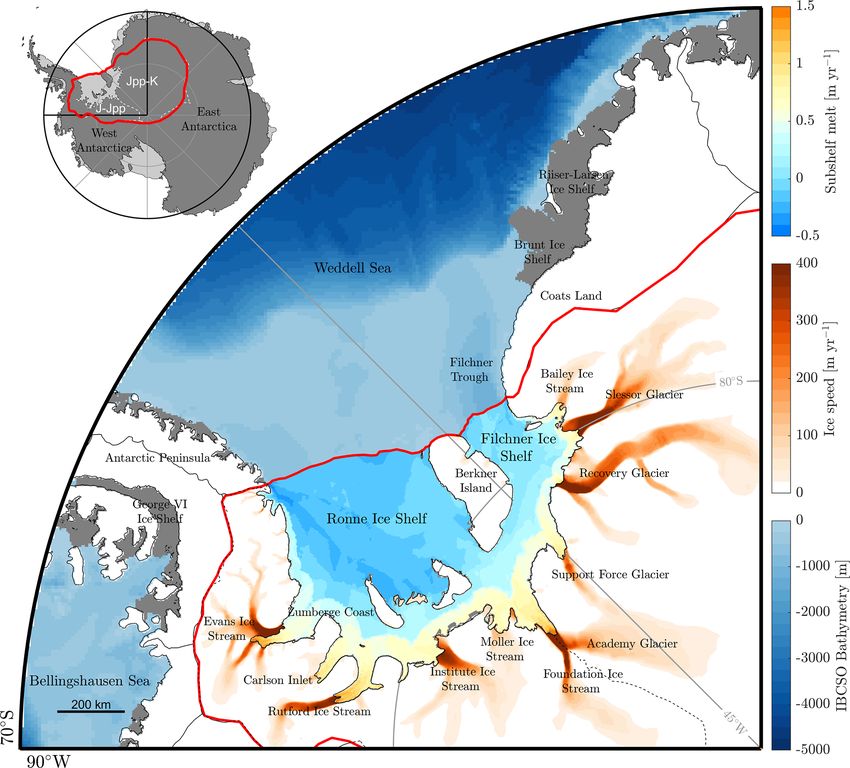
4676                                                                              E. A. Hill et al.: Filchner–Ronne sea level change

Figure 1. Map of Filchner–Ronne region. Our model domain is outlined in red. Orange to red shows model-calculated ice speeds [m yr−1 ]
initialized to observations using a model inversion with m = 3 and n = 3, over the grounded portion of the catchment. Blue to yellow shading
shows sub-shelf melt rates across the Filchner and Ronne ice shelves, using the ocean box melt parameterization with sample point estimates
for parameters from their probability distributions (see Appendix B). Light to dark blue shading shows sea floor depth from the IBCSO
dataset (Arndt et al., 2013). The inset map shows the full extent of our model domain (red) as well as the drainage basins (Jpp-K, J-Jpp) as
defined by Rignot et al. (2019) in white.

charges approximately 200 Gt yr−1 (Gardner et al., 2018) of             bayment (ASE): Jacobs et al., 2011; Jenkins et al., 2010;
sea-level-relevant ice mass into the surrounding ocean. Ice             Schmidtko et al., 2014). Warm water in the ASE has been
from the interior of the Antarctic Ice Sheet flows into the             linked to recent ice shelf thinning (Pritchard et al., 2012;
FRIS primarily via 11 fast-flowing ice streams (Fig. 1). These          Paolo et al., 2015), grounding line retreat (Rignot et al.,
ice streams are marine-based; i.e. their bed topography rests           2014), and increased ice discharge (Mouginot et al., 2014;
substantially below sea level, which has implications for ma-           Shepherd et al., 2018; Rignot et al., 2019). In contrast, wa-
rine ice sheet instability (Ross et al., 2012). Throughout this         ter entering the FRIS cavity is relatively cold (< 0 ◦ C), high-
paper we refer to the FR basin as the combined area of the              salinity shelf water, and as a result, sub-shelf melt rates are
two major drainage basins (Jpp-K, J-Jpp) as defined by Rig-             an order of magnitude lower than those in the ASE. The FR
not et al. (2019) that encompass a number of smaller ice                basin is also a region of Antarctica that has not undergone
stream catchments that drain into the FRIS.                             significant change during the modern observational period.
   Current mass loss from the Antarctic Ice Sheet is con-               Over the past 4 decades (1979–2017), the FR basin has re-
centrated in regions where warm circumpolar deep water                  mained relatively stable (accumulation is balanced by dis-
propagates on the continental shelf (e.g. Amundsen Sea Em-              charge) (Rignot et al., 2019), alongside a negligible change

The Cryosphere, 15, 4675–4702, 2021                                                          https://doi.org/10.5194/tc-15-4675-2021
E. A. Hill et al.: Filchner–Ronne sea level change                                                                            4677

(1–3 cm yr−1 ) in surface elevation (Shepherd et al., 2019) and     2   Uncertainty quantification
no significant long-term speed-up of the major ice streams
(Gudmundsson and Jenkins, 2009; Gardner et al., 2018).              Uncertainty quantification can be broadly defined as the sci-
   Recent work suggests that melt rates beneath the FRIS            ence of identifying sources of uncertainty and determining
could greatly increase in response to a tipping point in the        their propagation through a model or real-world experiment
neighbouring Weddell Sea. Studies have now shown that 21st          with the ultimate goal of quantifying, in probabilistic terms,
century changes in atmospheric conditions and sea ice con-          how likely an outcome or quantity of interest may be.
centration could redirect relatively warm deep water beneath           Early estimates of uncertainties in projections of future sea
the FRIS via the Filchner trough (Fig. 1: Hellmer et al.,           level change from the Antarctic Ice Sheet were derived from
2012, 2017; Hazel and Stewart, 2020). This would cause the          sensitivity studies that evaluated a small sample of a param-
FR cavity to switch from what is widely referred to as a            eter space directly in individual ice sheet models (e.g. De-
“cold state” to a “warm state”, similar to the ice shelf cav-       Conto and Pollard, 2016; Winkelmann et al., 2012; Golledge
ities (e.g. Pine Island and Thwaites) in the ASE. Ultimately,       et al., 2015; Ritz et al., 2015). Model intercomparison ex-
this warm water could be directed towards highly buttressed         periments have since been used to quantify uncertainties as-
regions of the ice shelf close to the grounding line (Reese         sociated with differences in the implementation of physical
et al., 2018a) via deep cavity bathymetry (e.g. Foundation Ice      processes between models, beginning with idealized set-ups
Stream: Rosier et al., 2018) and dramatically increase melt         (e.g. MISMIP and MISMIP+; Pattyn et al., 2012; Cornford
rates under the FRIS. A loss of resistive stress at the ground-     et al., 2015), and more recently on an ice sheet scale as
ing line as a result of ocean-induced melt could force dy-          part of the ISMIP6 project (Seroussi et al., 2020). Recently,
namic imbalance and grounding line retreat of the ice streams       the use of uncertainty quantification techniques has become
feeding the FRIS.                                                   more common for estimating uncertainties in projections of,
   Most previous studies have only assessed uncertainties in        for example, sea level rise, based on the current knowledge
sea level contribution, on an ice-sheet-wide scale, rather than     of uncertainties associated with model parameters or forc-
individual drainage basins (with the exception of Schlegel          ing functions (parametric uncertainty) (Edwards et al., 2019;
et al., 2018). These Antarctic-wide ensemble simulations            Schlegel et al., 2018, 2015; Bulthuis et al., 2019; Aschwan-
also rely on coarse grid resolution to be computationally fea-      den et al., 2019; Nias et al., 2019; Wernecke et al., 2020).
sible, and as a result they may not capture small-scale pro-        This includes techniques that weight model parameters and
cesses or accurate grounding line migration relevant on re-         outputs according to some performance measures, to provide
gional scales. Some studies have performed sensitivity ex-          a probabilistic assessment of sea level change (Pollard et al.,
periments on climate–ocean forcing on the FR basin (Corn-           2016; Ritz et al., 2015). Some of these studies have also
ford et al., 2015; Wright et al., 2014), but we do not know of      drawn upon statistical surrogate modelling techniques such
an uncertainty quantification assessment of the FR region’s         as Gaussian process emulators (Edwards et al., 2019; Pollard
potential contribution to sea level rise. A comprehensive un-       et al., 2016; Wernecke et al., 2020) or polynomial chaos ex-
certainty analysis is needed to fully understand the future of      pansions (Bulthuis et al., 2019) to mimic the behaviour of an
this region of Antarctica should it undergo an increase in sub-     ice sheet model and sample a much larger parameter space to
shelf melting.                                                      make predictions of Antarctic contribution to sea level rise.
   In this paper, we use an uncertainty quantification ap-             In this study, we are using a probabilistic approach, in
proach to assess the future of the FR basin to achieve three        which we are primarily interested in quantifying uncertain-
aims: (1) estimate potential mass change from the FR basin          ties in the forward propagation of input uncertainties that re-
through to the year 2300, (2) quantify the uncertainty asso-        late to parameters in the model or in the functions used to
ciated with mass change projections, and (3) identify param-        force climate warming, on a quantity of interest. We make
eters in our model or forcing functions that account for the        use of the MATLAB-based toolbox, UQLab, and the uncer-
majority of our projection uncertainty and should be prior-         tainty quantification framework of Sudret (2007), on which
ity areas for further research to constrain the spread of fu-       the MATLAB-based toolbox is based (Marelli and Sudret,
ture projections. To do this, we integrate an existing suite        2014). UQLab includes an extensive suite of tools encom-
of uncertainty quantification tools (UQLAB: Marelli and Su-         passing all necessary aspects of uncertainty quantification.
dret, 2014) for use with the state-of-the-art ice flow model        Here, we summarize the approach and tools used in this
Úa (Gudmundsson, 2020). See Fig. 2 for a summary of the             study (Fig. 2), and we refer the reader to the UQLAB docu-
method used in this paper. The paper is structured as fol-          mentation (https://www.uqlab.com/, last access: 29 Septem-
lows: in the following (Sect. 2) we introduce the uncer-            ber 2021, Marelli and Sudret, 2014) for further details.
tainty methodology used in this paper. In Sect. 3 we explain
the model set-up and input parameters that are propagated
through our forward model. Section 4 presents our proba-
bilistic projections and the results of our sensitivity analysis,
which are then discussed in Sect. 5.

https://doi.org/10.5194/tc-15-4675-2021                                                  The Cryosphere, 15, 4675–4702, 2021
4678 E. A. Hill et al.: Filchner–Ronne sea level change
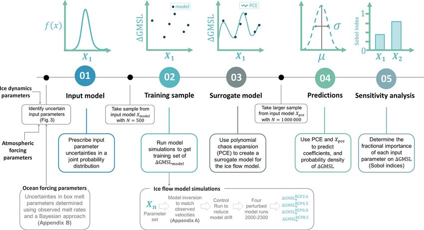
Figure 2. Workflow diagram summarizing the uncertainty quantification approach used in this study. We first identify uncertain input pa-
rameters and represent them in probabilistic framework. A training sample of 500 points is taken from this input parameter space and used
as input to an ensemble of simulations in our ice flow model, which we hereafter refer to as our “training ensemble”. Using this training
sample and the surrogate modelling capabilities in UQLAB we create a polynomial chaos expansion (PCE) that mimics the behaviour of our
ice flow model. This allows us to evaluate a much larger sample from our parameter space, and these surrogate models are used to derive
predictions and probability density functions for changes in global mean sea level (1GMSL). Finally, we use sensitivity analysis to identify
the proportional contribution of each input parameter on projection uncertainty.
We can think of a physical model (M) as a map from an values of some input parameters are changed, the relationship
input parameter space to an output quantity of interest, as between model inputs and model outputs may be approxi-
mated using a much simpler and computationally faster sur-
Y = M(X), (1)
rogate model. The uncertainty estimation can then be done in
where our uncertain input parameters are specified as a prob- a much more computationally efficient way using the surro-
abilistic input model (X) with a joint probability distribution gate model.
function X ∼ fX (x), and Y is a list of model responses. Us- Polynomial chaos expansion (PCE) is a surrogate mod-
ing this approach we are able to propagate the uncertainties elling technique that approximates the relationship between
in the inputs X to the outputs Y . We can think of our ice flow input parameters and output response in an orthogonal poly-
model in the same way, 1GMSL = Úa(X), where 1GMSL nomial basis. Aside from the work of Bulthuis et al. (2019),
is our model response or quantity of interest. In the following PCE surrogate modelling has not yet been used extensively
sections we outline eight uncertain input parameters that are by the glaciological community as a computationally effi-
represented in X. These relate to basal sliding and ice rhe- cient substitute for ice sheet models. The truncated PCE,
ology (Sect. 3.2), surface accumulation (Sect. 3.3), and sub- MPC (X), used to approximate the behaviour of our ice sheet
shelf melting (Sect. 3.4). Uncertainties in these input param- model M(X), takes the form
eters are defined in a probabilistic way based on the available X
information (Fig. 3). For parameters used to force sub-shelf M(X) ≈ MPC (X) = yα 9α (X), (2)
α∈A
melt rates, we conducted a separate Bayesian analysis to de-
termine their input parameter probability distributions (see where 9α (X) represents multivariate polynomials that are
Appendix B). orthonormal with respect to the joint input probability den-
Quantifying the uncertainty in model outputs due to uncer- sity function fX , A ⊂ NM is a set of multi-indices of the
tainty in input parameters or forcings may require a computa- multivariate polynomials 9α , and yα represents the coeffi-
tionally unfeasibly large number of model evaluations. How- cients. Here, our PCEs are calculated using the least angle
ever if, for example, the model response varies slowly as the regression (LAR) algorithm in UQLab (Blatman and Sudret,
The Cryosphere, 15, 4675–4702, 2021 https://doi.org/10.5194/tc-15-4675-2021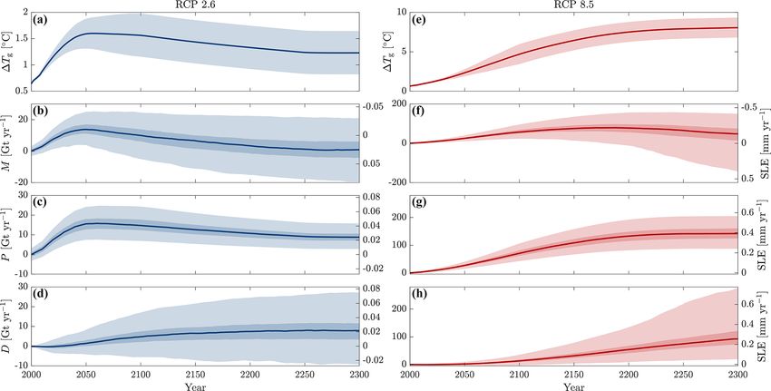
E. A. Hill et al.: Filchner–Ronne sea level change 4679
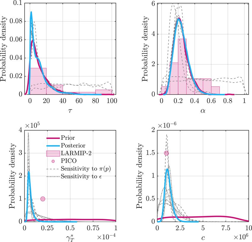
Figure 3. Probability distributions for uncertain parameters included in our analysis, grouped by ice dynamics (blue rectangle), atmospheric
forcing (green rectangle), and ocean forcing (orange rectangle). For each parameter, x axes show the parameter bounds, and red lines show
the probability distribution functions. Yellow circles show the sample point estimates for each of our parameters. The distributions of the
four ocean forcing parameters are outputs from our Bayesian analysis (Appendix B) in which we optimized the parameter distributions using
observations of melt rates beneath the Filchner–Ronne ice shelf.
2011; Marelli and Sudret, 2019) that solves a least-square improved understanding is needed to constrain future projec-
minimization problem. This algorithm iteratively moves re- tions. Here, we are using Sobol indices which are a variance-
gressors from a candidate set to an active set, and at each based method where the model can be expanded into sum-
iteration a leave-one-out (LOO) cross-validation error is cal- mands of increasing dimension, and total variance in model
culated. After all iterations are complete, the best sparse can- output can be described as the sum of the variances of these
didate basis is that with the lowest leave-one-out error. This is summands.
designed to reduce the potential for over-fitting and reduced First-order indices (Si ), often also referred to as “main ef-
accuracy when making predictions outside of the training set. fects”, are the individual effect of each input parameter (Xi )
This sparse PCE calculation in UQLab also uses the LOO on the variability in the model response (Y ), defined as
error for (1) adaptive calculation of the best polynomial de-
Var[E(Y |Xi )]
gree based on the experimental design and (2) adaptive q- Si = . (5)
norm setup for the truncation scheme. For further details on Var(Y )
the PCE algorithm see Marelli and Sudret (2019). We also Total Sobol indices (SiT ) are then the sum of all Sobol in-
outline details on how input uncertainties were propagated dices for each input parameter and encompass the effects of
through our model to create our PCE in Sect. 3.5. parameter interactions. Values for Sobol indices are between
Once the surrogate model has been created, the moments 0 and 1, where large values of Si indicate parameters that
of the PCE are encoded in its coefficients where the mean strongly influence the projections of global mean sea level.
(µPC ) and variance (σ PC )2 are as follows If Si ≈ SiT , then it can be assumed that the effect of parame-
ter interactions is negligible.
µPC = E[MPC (X)] = y0 , (3)
X These Sobol indices can be calculated analytically from
PC 2 PC PC 2
(σ ) = E[(M (X) − µ ) ] = yα2 . (4) our existing PCEs, by expanding portions of the polyno-
α∈A mial that depend on each input variable to directly calculate
α6=0
parameter variance using the PCE coefficients. Each of the
Our existing PCE surrogate models can additionally be summands of the PCE can be expressed as
used in a sensitivity analysis to quantify the proportional X
fv (xv ) = yα 9α (X). (6)
contribution of parametric uncertainty on projections of
α∈Av
1GMSL. This allows us to identify input parameters where
https://doi.org/10.5194/tc-15-4675-2021 The Cryosphere, 15, 4675–4702, 2021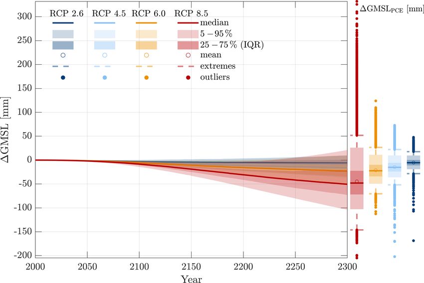
4680                                                                          E. A. Hill et al.: Filchner–Ronne sea level change

   Due to the orthonormality of the basis, the variance of our      We also impose a minimum thickness constraint of 30 m us-
truncated PCE reads as                                              ing the active-set method to ensure that ice thicknesses re-
                  X                                                 main positive. Throughout all simulations our calving front
Var[MPC (X)] =       yα2 ,                                 (7)      remains fixed in its originally prescribed position. At the end
                    α∈A                                             of each forward simulation we calculate the final change in
                    α6=0
                  X                                                 global mean sea level (1GMSL) as the ice volume above
Var[fv (xv )] =           yα2 .                              (8)
                                                                    flotation that will contribute to sea level change based on the
                  α∈Av
                   α6=0                                             area of the ocean (Goelzer et al., 2020).

   The first-order Sobol indices in Eq. (5) are then calculated     3.2   Basal sliding and ice rheology
as the ratio between the two terms above.
                                                                    There are two components of surface glacier velocities: inter-
                                                                    nal deformation and basal sliding. Úa uses inverse methods
3     Methods                                                       to optimize these velocity components based on observations
                                                                    by estimating the ice rate factor (A) in Glen’s flow law and
3.1    Ice flow model
                                                                    basal slipperiness parameter (C) in the sliding law. This sec-
Here we use the vertically integrated ice flow model Úa             tion introduces uncertainties related to the exponents of the
(Gudmundsson, 2020) to solve the ice dynamics equations             flow law and basal sliding law, whereas details of the inverse
using the shallow-ice stream approximation (SSTREAM),               methodology are included in Appendix A.
also commonly referred to as the shallow-shelf approx-                 Glen’s flow law (Glen, 1955) is used to relate strain rates
imation (SSA) and the “shelfy-stream” approximation.                and stresses as a simple power relation
(MacAyeal, 1989). Úa has been used in previous studies on           ˙ij = Aτen−1 τij ,                                         (9)
grounding line migration and ice shelf buttressing and col-
lapse (De Rydt et al., 2015; Reese et al., 2018b; Gudmunds-         where ˙ij are the elements of the strain rate tensor, τe is ef-
son et al., 2012; Gudmundsson, 2013; Hill et al., 2018), and        fective stress (second invariant of the deviatoric stress ten-
model results have been submitted to a number of intercom-          sor), τij are the elements of the deviatoric stress tensor, A
parison experiments (Pattyn et al., 2008, 2012; Levermann           is the temperature-dependent rate factor, and n is the stress
et al., 2020; Cornford et al., 2020).                               exponent.
   Our model domain extends across the two major drainage              This stress exponent (n) controls the degree of non-
basins that feed into the FRIS (Fig. 1). Within this domain,        linearity of the flow law, and most ice flow modelling stud-
we generated a finite-element mesh (Fig. S1 in the Supple-          ies adopt n = 3, as it is considered applicable to a num-
ment) with ∼ 92 000 nodes and ∼ 185 000 linear elements             ber of regimes (see review in Cuffey and Paterson, 2010).
using the Mesh2D Delaunay-based unstructured mesh gen-              However, experiments reaching high stresses (Kirby et al.,
erator (Engwirda, 2015). Element sizes were refined based           1987; Goldsby and Kohlstedt, 2001; Treverrow et al., 2012),
on effective strain rates and distance of the grounding line        or analysing borehole measurements and ice velocities (e.g.
and have a maximum size of 27 km, a median size of 2 km,            Gillet-Chaulet et al., 2011; Cuffey and Kavanaugh, 2011;
and a minimum size of 660 m. Within a 10 km distance of             Bons et al., 2018), have suggested that n > 3. It is also possi-
the grounding line elements are 3 km and refined further to         ble that at low stresses, the creep regime may become more
900 m within a distance of 1.5 km. Outside of our uncer-            linear n < 3 (Jacka, 1984; Pettit and Waddington, 2003; Pet-
tainty analysis, we tested the sensitivity of our results to mesh   tit et al., 2011), which is supported by ice shelf spreading
resolution by repeating our median and maximum 1GMSL                rates n = 2–3 (Jezek et al., 1985; Thomas, 1973). While it
simulations under RCP8.5 forcing and dividing or multiply-          can be considered that n = 3 is appropriate in most dynam-
ing the aforementioned element sizes by 2. Our results are          ical studies, the exact numerical value is not known and it
largely insensitive to the mesh resolution, with a percentage       appears plausible that it can range between 2 and 4. To cap-
deviation in 1GMSL of only 3 % by 2300. Finally, we lin-            ture the uncertainty in the stress exponent, we take n ∈ [2, 4]
early interpolated ice surface, thickness, and bed topography       and sample continuously from a uniform distribution within
from BedMachine Antarctica v1 (Morlighem et al., 2020)              this range (Fig. 3).
onto our model mesh. We initialize our model to match ob-              Basal sliding is considered the dominant component of
served velocities using an inverse approach (see Sect. 3.2 and      surface velocities in fast-flowing ice streams. The Weertman
Appendix A).                                                        sliding law is defined as
   During forward transient simulations, Úa allows for fully        τb = C −1/m kvb k1/m−1 vb ,                                (10)
implicit time integration, and the non-linear system is solved
using the Newton–Raphson method. Úa includes automated              where C is a basal slipperiness coefficient and vb the basal
time-dependent mesh refinement, allowing for high mesh              sliding velocity. The Weertman sliding law typically cap-
resolution around the grounding line as it migrates inland.         tures hard-bed sliding, in which case m = n and is normally

The Cryosphere, 15, 4675–4702, 2021                                                       https://doi.org/10.5194/tc-15-4675-2021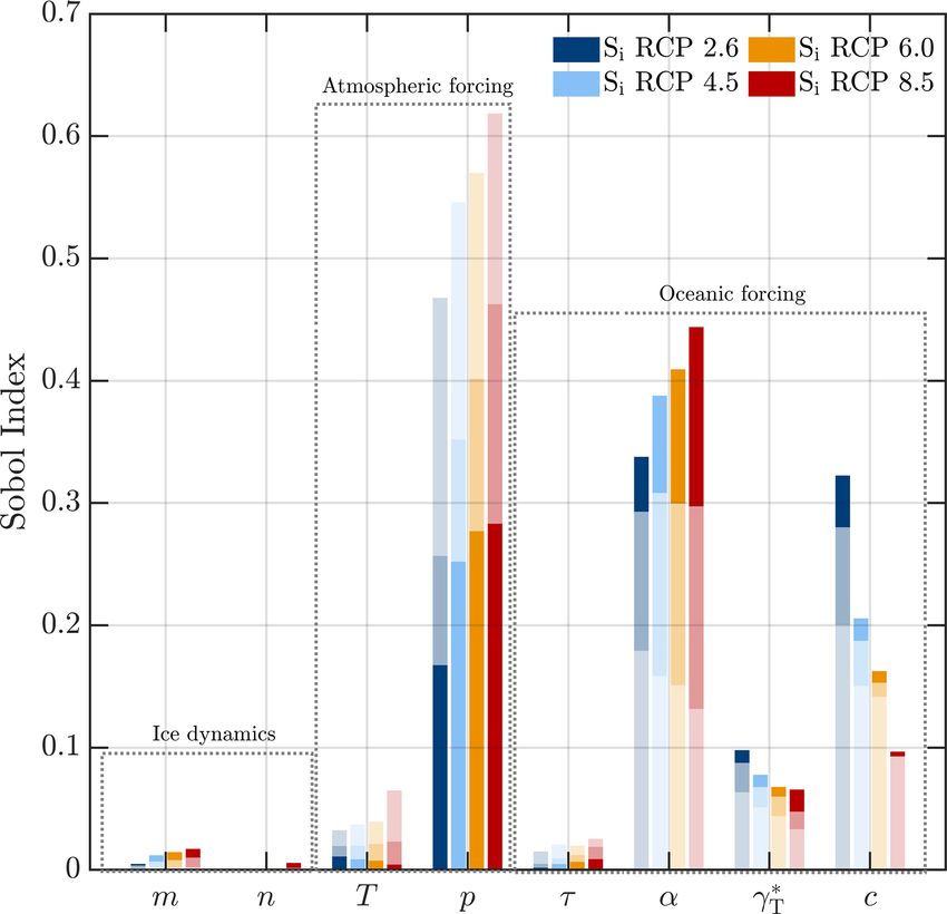
E. A. Hill et al.: Filchner–Ronne sea level change                                                                               4681

set equal to 3 (Cuffey and Paterson, 2010). However, using
different values for m alters the non-linearity of the sliding
law and can thus be used to capture different sliding pro-
cesses, i.e. viscous flow for m = 1 and plastic deformation
for m = ∞. There are limited in situ observations of basal
conditions, and the value of m relies on numerical estimates
of basal sliding based on model fitting to observations.
    A number of studies have tested different values of m to
fit observations of grounding line retreat or speed-up at Pine
Island Glacier (Gillet-Chaulet et al., 2016; Joughin et al.,
2010; De Rydt et al., 2021). These studies show that m = 3
can underestimate observations, and more plastic-like sliding
(m > 3) is needed in at least some parts of the catchment to
replicate observations (Joughin et al., 2010; De Rydt et al.,
2021). This uncertainty in the value of m can ultimately af-       Figure 4. Changes in global mean temperatures (1Tg [◦ C]) relative
fect projections of sea level rise (Ritz et al., 2015; Bulthuis    to pre-industrial levels for four Representative Concentration Path-
et al., 2019; Alevropoulos-Borrill et al., 2020) by altering the   ways (RCPs) 2.6 (blue), 4.5 (green), 6.0 (yellow), and 8.5 (pink).
length and time taken for perturbations (e.g. ice shelf thin-      Shading shows uncertainty regions between the 25th and 75th per-
ning or grounding line retreat) to propagate inland.               centiles.
    While additional sliding laws have been proposed and are
now implemented within a number of existing ice flow mod-          the atmosphere–ocean general circulation model emulator
els, in this study we use the Weertman sliding law, as it re-      MAGICC6.0 (http://live.magicc.org, last access: 29 Septem-
mains the most common. This narrows the parameter space,           ber 2021: Meinshausen et al. (2011)). For each RCP scenario
allowing us to fully integrate the influence of m on projec-       we obtain 600 (historically constrained) model simulations
tions of future sea level rise into our uncertainty assessment     between 2000 and 2100 (see Meinshausen et al. (2009) for
(by performing an inverse model run prior to each perturbed        details on the probabilistic set-up). We then use the ensem-
run; see Sect. 3.5). This is an advancement over previous          ble median and uncertainty bounds within a “very likely”
Antarctic-wide studies, which given domain size have no            range between the 25th and 75th percentiles. To extend the
choice but to invert the model for a handful of different m        record to 2300, we use a single model realization, using the
values prior to uncertainty propagation (e.g. Bulthuis et al.,     default climate parameter settings used to produce the RCP
2019; Ritz et al., 2015). To capture uncertainty in m and          greenhouse gas concentrations for each RCP scenario (Mein-
to sample from a range of possible methods of basal slip,          shausen et al., 2009) and keep the upper and lower bounds
we take m ∈ [2, 9] and sample from a uniform distribution          constant from 2100 to 2300 (Fig. 4). Uncertainty in projec-
(Fig. 3).                                                          tions from 2100 to 2300 may well be larger, but we choose
                                                                   not to make an assumption on how errors will propagate up
3.3   Surface accumulation                                         to 2300. Global temperatures from MAGICC 6.0 were also
                                                                   used in the Antarctic linear response model inter-comparison
To capture uncertainties in future climate forcing, we use         (LARMIP-2) experiment (Levermann et al., 2020) and are
projections from four Representative Concentration Path-           consistent with projections used in other Antarctic-wide sim-
ways (RCPs) presented in the Fifth Assessment Report of the        ulations (Bulthuis et al., 2019; Golledge et al., 2015).
Intergovernmental Panel on Climate Change (IPCC). These               Following the work of a number of previous studies
pathways capture plausible changes in anthropogenic green-         (e.g. Pattyn, 2017; Bulthuis et al., 2019; DeConto and Pol-
house gas emissions for the 21st and 22nd centuries. RCP2.6        lard, 2016; Garbe et al., 2020), global temperature changes
is a strongly mitigated scenario, and multi-model mean es-         (1Tg ) are used to force annual changes in surface mass bal-
timates from the IPCC report (IPCC, 2014) project a global         ance through our forward-in-time simulations, by prescribing
temperature increase of less than 2 ◦ C above pre-industrial       changes in surface temperature (Tair ) and precipitation (P ) as
levels by 2100 and is the goal of the 2016 Paris Agree-            follows:
ment. Two intermediate scenarios (RCP4.5 and RCP6.0) rep-
                                                                            air
resent global temperature increases of ∼ 2.5 and ∼ 3 ◦ C with      Tair = Tobs  − γ (s − sobs ) + 1Tg ,                           (11)
reductions in emissions after 2040 and 2080, respectively          P                              air
                                                                       = Aobs × exp(p · (Tair − Tobs  )),                         (12)
(IPCC, 2014). Finally, RCP8.5 projects a global temperature
increase of ∼ 4.5 ◦ C by 2100 and is now often referred to as               air and A
                                                                   where Tobs        obs are surface temperatures and accumula-
an “extreme” or “worst-case” climate change scenario.              tion rates from RACMO2.3, respectively (Van Wessem et al.,
   Global mean temperature changes (1Tg ) from 1900 to             2014). Temperature changes through time are corrected for
2300 relative to pre-industrial levels were obtained from          changes in surface elevation (s) from initial observations

https://doi.org/10.5194/tc-15-4675-2021                                                   The Cryosphere, 15, 4675–4702, 2021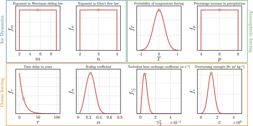
4682                                                                       E. A. Hill et al.: Filchner–Ronne sea level change

(sobs ), using a lapse rate of γ = 0.008 ◦ C m−1 (Pattyn, 2017;    a uniform distribution (Fig. 3). While the lower bound of
DeConto and Pollard, 2016), and subsequently used to force         this range sits below what is expected from the Clausius–
changes in precipitation using an expected percentage in-          Clapeyron relationship, it is able to capture low rates of sur-
crease in precipitation (p) per degree of warming (Aschwan-        face mass balance that could occur with some (albeit limited)
den et al., 2019). This captures the rise in snowfall expected     increases in surface runoff and melt under RCP8.5 forcing.
with the increased moisture content of warmer air, suggested
by climate models (e.g. Palerme et al., 2017; Frieler et al.,      3.4   Sub-shelf melt
2015). Here, we do not implement a positive-degree-day sur-
face melt model. While it is possible that RCP8.5 forcing          Ice shelf thinning due to ocean-induced melt can reduce
in particular could cause enhanced surface melting in some         buttressing forces on grounded ice and accelerate ice dis-
regions of Antarctica, due to the southern location of the         charge. Such feedbacks may already be taking place in parts
Filchner–Ronne ice shelf, surface melt and runoff are un-          of West Antarctica. However, future changes in ocean con-
likely to outweigh increases in snowfall in the high-warming       ditions remain uncertain, owing to poor understanding and
scenario (Kittel et al., 2021).                                    the challenges of modelling interactions between global at-
   To capture further uncertainties associated with atmo-          mospheric warming and ocean circulation and temperature
spheric forcing, we introduce two uncertain parameters into        changes (Nakayama et al., 2019; Thoma et al., 2008). In par-
our analysis: (1) a scaling factor to select a temperature re-     ticular, the likelihood that the Filchner–Ronne ice shelf cav-
alization between the 25th and 75th percentiles of the en-         ity will be flushed with modified warm deep water in the fu-
semble median temperature for each RCP scenario (Fig. 4)           ture is unclear (Hellmer et al., 2012).
and (2) uncertainty in the expected changes in precipitation          To parameterize basal melting beneath the ice shelf, we
across the Antarctic Ice Sheet with increased air tempera-         use an implementation of the PICO ocean box model (Reese
tures.                                                             et al., 2018a) for use in Úa, which we hereafter refer to
   First, instead of only using the ensemble median change         as the ocean box model. This provides a computationally
in temperature for each RCP scenario, we capture the spread        feasible alternative to fully coupled ice–ocean simulations
within each forcing scenario by incorporating a temperature        for large ensemble analysis, which is more physically based
scaling parameter (T ) as follows: 1Tg (n) = 1Tgmedian + T ·       than simple depth-dependent parameterizations (e.g. Favier
                                                                   et al., 2014) and has been shown to provide similar results
Tgerr , where for each RCP scenario 1Tgmedian is the median,
                                                                   to coupled simulations under future climate forcing scenar-
1Tgerr is the distance either side of the median within the 25th
                                                                   ios (Favier et al., 2019). The basic overturning circulation in
and 75th percentiles, and 1Tg (n) is the resultant temperature
                                                                   ice shelf cavities is captured using a series of ocean boxes,
realization used to force both surface accumulation (P ) and
                                                                   calculated based on their distance from the grounding line.
ocean temperature (see Sect. 3.4). We assume that there is de-
                                                                   The overturning flux q is then calculated as the density dif-
creasing likelihood of temperature profiles further away from
                                                                   ference between the far-field (p0 ) and grounding line (p1 )
the median, and so we prescribe a Gaussian distribution for
                                                                   water masses using a constant overturning strength param-
T between −1 (25th percentile) and 1 (75th percentile) and
                                                                   eter (c). The melt parameterization also includes a turbu-
centred around 0 (median: Fig. 3).
                                                                   lent heat exchange coefficient γT∗ that controls the strength
   Secondly, we capture uncertainty associated with precip-
                                                                   of melt rates by varying the heat flux across the ice–ocean
itation by varying the amount by which precipitation in-
                                                                   boundary. For a detailed description of the physics of the
creases per degree of warming (p). While it is generally ac-
                                                                   PICO box model, see Reese et al. (2018a). To calculate sub-
cepted that accumulation will increase with future warming,
                                                                   shelf melt rates, the box model requires inputs of sea-floor
the value of p remains uncertain. Snow accumulation could
                                                                   temperature (Tocean ) and salinity (S) on the continental shelf
prevent runaway ice discharge from the Antarctic Ice Sheet,
                                                                   to drive the ocean cavity circulation. We use S = 34.65 psu
which means that parameterizations of precipitation increase
                                                                   and the initial observed ocean temperature for the Weddell
with warming have implications for accurate projections of                ocean = −1.76 ◦ C from Schmidtko et al. (2014), which
                                                                   Sea Tobs
mass change across the ice sheet. Previous studies using ice
                                                                   was proposed for use in PICO (Reese et al., 2018a). For
core records, historical global climate model (GCM) simu-
                                                                   the FR basin we use five ocean boxes and only apply sub-
lations, and future GCM simulations as part of the CMIP5
                                                                   shelf melting to nodes that are fully afloat (no connecting
ensemble have estimated anywhere between 3.7 %–9 % in-
                                                                   grounded nodes) to avoid overestimating grounding line re-
crease in Antarctic accumulation per degree of warming
                                                                   treat (Seroussi and Morlighem, 2018).
(Krinner et al., 2007, 2014; Gregory and Huybrechts, 2006;
                                                                      To force changes in sub-shelf melt rates using RCP
Bengtsson et al., 2011; Ligtenberg et al., 2013; Frieler et al.,
                                                                   forcing, we update the far-field ocean temperature (Tocean )
2015; Palerme et al., 2017; Monaghan et al., 2008). To cap-
                                                                   through time with an ocean temperature anomaly:
ture this range of possible values for (p), we sample from
p ∈ [4, 8] and make no assumption of the distribution (like-                 ocean
                                                                   Tocean = Tobs   + 1To .                                   (13)
lihood) of the value of p within this range by sampling from

The Cryosphere, 15, 4675–4702, 2021                                                   https://doi.org/10.5194/tc-15-4675-2021
E. A. Hill et al.: Filchner–Ronne sea level change 4683
It is often assumed that atmospheric temperature changes sign (training set) for the surrogate model. An input param-
1Tg can be translated to ocean temperature changes 1To eter sample of 500 points was extracted from the parameter
using some scaling factor (α) (Maris et al., 2014; Golledge space using Latin hypercube sampling. This sample was de-
et al., 2015; Levermann et al., 2014, 2020). Here, we use the termined to be sufficient in size such that the mean 1GMSL
linear scaling proposed in Levermann et al. (2020), which had converged for each RCP surrogate model (see Fig. S3).
additionally includes a time delay τ to capture the assumed Using each training sample, we then evaluate the ice flow
time lag between atmospheric and subsurface ocean warm- model to generate model responses. For each sample point
ing. we perform six model runs. First, we perform a model in-
version following the procedure outlined in Appendix A us-
1To = α · 1Tg (t − τ ) (14) ing the selected values for m and n. The resulting optimized
To obtain suitable values for α and τ , Levermann et al. fields of C and A are then input into five forward-in-time
(2020) used 600 atmospheric temperature realizations (also simulations, four based on different RCP scenarios and one
from MAGICC6.0 simulations) and ocean temperatures from control run, all of which run from 2000 (nominal start year)
19 CMIP5 models (Taylor et al., 2012) to derive the relation to 2300.
between global surface temperatures and subsurface ocean Experience has shown that our model (similar to others,
warming by computing the correlation coefficient (α) and e.g. Bulthuis et al., 2019; Schlegel et al., 2018) undergoes
time delay between the signals (τ ). The values proposed are a period of model drift at the start of the simulation, char-
consistent with α ≈ 0.25 used in a number of other Antarctic- acterized by a slowdown and thickening of many of the ice
wide simulations (Bulthuis et al., 2019; Golledge et al., 2015; streams in our domain, amounting to between 80 and 100 mm
Maris et al., 2014). However, given the spread of values de- of negative contribution to 1GMSL. We found model drift to
pending on the choice of CMIP5 model, no single value for be similar between parameter sets, but it was affected by the
either α or τ can be chosen with confidence, and it is instead basal boundary conditions from our inversion. Hence, rather
appropriate to sample from parameter probability distribu- than specify a single baseline for the entire experimental de-
tions. sign, we perform a control simulation for each set of basal
We identify a further two uncertain parameters in the boundary conditions. This control run uses selected values
ocean box model that additionally control the strength of sub- of m and n and inverted fields of C and A but holds all
shelf melt. These are the turbulent heat exchange coefficient other input parameters fixed to their sample point estimates,
γT∗ and the strength of the overturning circulation c. Values as well as using a constant temperature forcing. Each control
for these parameters presented in Reese et al. (2018a) have run is followed by four forward runs, one for each RCP forc-
been optimized to present-day ocean temperatures and ob- ing scenario, in which surface accumulation and sub-shelf
servations of melt rates for a circum-Antarctic set-up. While melt rates are updated at annual intervals based on global
upper and lower bounds for these parameters have also been temperature changes (Fig. 4). The final calculated change in
proposed (Reese et al., 2018a; Olbers and Hellmer, 2010), global mean sea level for each RCP scenario is with respect
little information exists on the likelihood of parameter val- to the preceding control run (1GMSLrcp − 1GMSLctrl ). For
ues within these ranges, particularly for different regions of our 500-member training ensemble, we perform 500 model
Antarctica, with varying ocean conditions. inversions and 2500 forward simulations.
For the four parameters that control the sub-shelf melt Model responses (1GMSL) and input parameter samples
rates (α, τ , γT∗ , and c), we decided to constrain their uncer- X = xi , . . ., xN are used to train four surrogate models (one
tainty (probability distributions) using a Bayesian approach. for each RCP scenario). This is done using the Polynomial
Using the a priori information on the distributions for α and Chaos module in UQLab (Marelli and Sudret, 2019) using
τ (Levermann et al., 2020) and possible upper and lower the LAR algorithm previously described in Sect. 2. We allow
bounds for γT∗ and c from Reese et al. (2018a) and Olbers the LAR algorithm to choose a PCE with a degree anywhere
and Hellmer (2010), alongside observed sub-shelf melt rates between 3 and 15 and q-norm between 0.1 and 1. Predic-
from Moholdt et al. (2014), we derive optimized posterior tions (mean and variance) of 1GMSL are then directly ex-
probability distributions for use as input to our uncertainty tracted from each surrogate model. To estimate the accuracy
propagation. The details of this are outlined in Appendix B, of our PCE predictions and and to calculate the quantiles of
and the resultant probability distribution functions for these our projections, we use bootstrap replications. We use 1000
parameters are shown in Fig. 3. replications (B) each with the same number of sample points
as the original experimental design (500) to create an addi-
3.5 Propagating uncertainty tional set of B PCEs and associated responses. Quantiles (5th
and 95th) were extracted from the bootstrap evaluations (see
In this section we explain how uncertainties in the input pa- Fig. S2). To assess the performance of our surrogate model,
rameters introduced in the previous sections are propagated we generated an additional and independent validation sam-
through our model to obtain projections of global mean sea ple of 20 sample points in the parameter space, evaluated for
level (Fig. 2). We began by generating an experimental de- each RCP scenario (total of 80 perturbed simulations). We
https://doi.org/10.5194/tc-15-4675-2021 The Cryosphere, 15, 4675–4702, 20214684 E. A. Hill et al.: Filchner–Ronne sea level change
responses, and calculated probability distributions using ker-
nel density (Fig. 5).
Our projections indicate it is most likely that the FR
basin will undergo limited change or contribute negatively
to global mean sea level by the year 2300. Under the
lowest-warming scenario (RCP2.6: 0.77–1.7 ◦ C), 1GMSL
is limited, ranging between −19.1 mm (5th percentile) and
9.57 mm (95th percentile: Table 1). The probability distri-
bution (Fig. 5) takes a near-to-normal shape, with a median
projection close to zero (−5.49 mm), but it has a weak pos-
itive skew of 0.16 (calculated using the moment coefficient
of skewness), with a tail extending towards a maximum sea
level contribution of ∼ 50 mm. Projections of 1GMSL under
the medium-warming scenarios RCP4.5 and 6.0 range from
−36.1 to 9.7 and −49.6 to 11.1 mm, respectively (Table 1).
These distributions are more positively skewed than RCP2.6
(skewness coefficients of 0.29 and 0.39, respectively), with
tails extending towards ∼ 100 mm of global sea level rise
(Fig. 5). Extreme warming leads to the greatest uncertainty in
projections, which range from −103 to 26 mm under RCP8.5
(Table 1). The median projection indicates a greater negative
contribution to sea level rise under higher warming. How-
ever, the probability distribution is asymmetric, with a long
tail (high positive skew = 0.77) that decreases exponentially
away from the median and reaches a maximum 1GMSL of
332 mm (Fig. 5). This long tail represents the potential for
low-probability but high-magnitude contributions to sea level
rise.
Figure 5. Probability density (a) and cumulative probability den- As our surrogate modelling is based around a single quan-
sity (b) for projections of change in global mean sea level tity of interest (1GMSL at the year 2300) it does not al-
(1GMSL) in millimetres by the year 2300 under four RCP emis- low us to evaluate temporal changes in ice loss directly. Fig-
sions scenarios. Dashed lines show the 5th, 50th, and 95th per- ure 6 instead presents projections through time from our 500-
centiles for the highest emission scenario RCP8.5. member training ensemble alongside the final 1GMSL from
each surrogate model (PCE). We also generate two additional
surrogate models for each RCP scenario at the years 2100
then calculate the root mean square error (RMSE) between and 2200 (Table 1) to evaluate projections at these time inter-
validation responses Yval to those calculated by each surro- vals, and we identify the temporal importance of parameters
gate model (YPCE ) using the same validation input parame- on projection uncertainty (see Sect. 4.2 and Fig. 7).
ter sample Xval . Predictions made by the surrogate models Both Table 1 and Fig. 6 show that the contribution to
are close to the responses by our ice flow model and have a 1GMSL and associated uncertainties increase through time.
maximum RMSE of 2.3 mm for our RCP8.5 surrogate model Within the next 100 years (up to 2100) we project little
(Fig. S2). change in ice mass from the FR basin. This constitutes a
small negative contribution to sea level rise of < 10 mm in
4 Results all warming scenarios (Table 1), with a maximum range of
−14.1 to 0.11 mm. By 2200 the spread of 1GMSL has di-
4.1 Projections of sea level rise from FR basin verged based on warming scenario, with little change un-
der limited forcing (RCP 2.6 = −5.05) and a greater nega-
We begin by presenting probabilistic projections of global tive contribution under higher warming (−30.2 in RCP8.5).
mean sea level change from the Filchner–Ronne basin for Between 2200 and 2300 uncertainties increase dramatically
four RCP scenarios. These projections were derived from in all warming scenarios, particularly in RCP8.5. Box plots
surrogate models that were trained with our 500 member in Fig. 6 show the projections generated from our surrogate
training ensemble of forward-in-time ice flow model sim- model in 2300 alongside our ice flow model training ensem-
ulations. We then evaluated these surrogate models with a ble. This shows that the probability distributions in the most
1 000 000 point sample (generated using Latin hypercube likely range between 5 %–95 % generated from our surrogate
sampling) from our input parameter space to derive model models are largely similar to those found from our training
The Cryosphere, 15, 4675–4702, 2021 https://doi.org/10.5194/tc-15-4675-2021E. A. Hill et al.: Filchner–Ronne sea level change 4685
Table 1. Contribution to global mean sea level (mm) at the years 2100, 2200, and 2300. The first number is the median projection, and values
in brackets are 5 %–95 % confidence intervals
2100 2200 2300
RCP2.6 −3.2(−6.4, 0.113) −5.05(−13.2, 3.86) −5.49(−19.1, 9.57)
RCP4.5 −4.99(−8.96, −0.975) −11(−22.7, 1.87) −15.1(−36.1, 9.7)
RCP6.0 −5.41(−9.51, −1.3) −15.4(−29.7, 0.204) −22.3(−49.6, 11.1)
RCP8.5 −8.39(−14.1, −2.99) −30.2(−55.2, −3.42) −48(−103, 26)
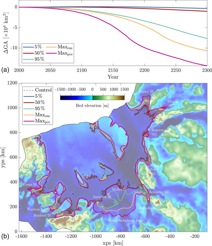
Figure 6. Projections of changes in global mean sea level (1GMSL) from 2000 and 2300 from our training ensemble of ice flow model
simulations. Dark shading is the interquartile range (IQR) defined between the 25th and 75th percentiles. Lighter shading shows the 5th–95th
percentiles. Box plots show the projections from the surrogate models (1GMSLPCE ) for each RCP scenario at 2300. Extreme values are
located at 1.5 times the interquartile range away from the 25th and 75th percentiles. Values outside of these extreme bounds are considered
to be outliers.
ensemble in 2300. However, we note that the tails of these 4.2 Parametric uncertainty
distributions, in particular for RCP8.5, extend substantially
beyond the maximum 1GMSL shown from our training en-
semble alone (150 mm). While this is expected with more In this section we present the results of our sensitivity analy-
extensive sampling of our parameter space, we test the feasi- sis, in which we determine how uncertainties in our input pa-
bility of 1GMSL = 332 mm by taking the parameter values rameters (parametric uncertainty) impact our projections of
that led to this and re-evaluating the “true” ice flow model. 1GMSL. To do this, first-order Sobol indices were decom-
This gives a slightly lower value of 1GMSL = 250 mm but posed from each of our PCE models (four RCP forcing sce-
one that is still considerably higher than in our original train- narios) and for three time steps: 2100, 2200, and 2300, which
ing ensemble despite its relatively large size (N = 500). This are presented in Fig. 7. We additionally assessed the individ-
demonstrates the benefits of our surrogate modelling ap- ual parameter-to-projection relationship, by re-evaluating our
proach, as it was able to capture the possibility of more surrogate model for each parameter, while all other parame-
extreme sea level rise scenarios that were not exposed by ters were held at their sample point estimates (see Fig. S4).
the original sample. Recalculating the surrogate model for By 2300 (dark shaded bars in Fig. 7) uncertainties in our
RCP8.5 including this “extreme” sample point reduces the four ocean forcing parameters collectively have the great-
maximum contribution to sea level rise to 288 mm. est fractional contribution to the uncertainty in our projec-
tions of global mean sea level contribution. This ranges from
60 % in RCP8.5 to 75 % for RCP2.6. Projection uncertainty
https://doi.org/10.5194/tc-15-4675-2021 The Cryosphere, 15, 4675–4702, 20214686 E. A. Hill et al.: Filchner–Ronne sea level change Figure 7. First-order Sobol indices, i.e. the fractional contribution of each input parameter on the uncertainty in our projections of 1GMSL, for each RCP forcing scenario. Dark shading shows the Sobol indices for 1GMSL in 2300. Two lighter shading colours represent Sobol indices at the years 2100 and 2200, to show the variability in parameter importance through time. in all RCP scenarios is primarily driven by ocean tempera- any other parameter (Fig. S4) and encompasses almost all of ture forcing and the value of α used to scale atmospheric to the 5 %–95 % spread of projections (Table 1). ocean temperatures. Uncertainties attributed to α appear to Of our two ocean box model parameters, overturning increase both with warming scenario and through time. In all strength (c) accounts for more projection uncertainty than RCP scenarios, fractional uncertainty associated with α in- the turbulent heat exchange coefficient (γT∗ ) in all warm- creases from 2100 to 2300 (light shaded bars in Fig. 7), coin- ing scenarios. This is consistent with the theory that sub- cident with an increase in the spread of 1GMSL contribution shelf melting at large and cold cavity ice shelves is predomi- (Fig. 6). In 2100, α has a greater impact on projection un- nantly driven by overturning strength (Reese et al., 2018a). certainty in the lower-warming scenario. However, by 2300, The fractional importance of c has the greatest variability the fractional uncertainty is greatest in RCP8.5, accounting between forcing scenarios than any other parameter. Un- for almost half of projection uncertainty (0.44) compared to like α, uncertainty associated with c decreases with warming, 0.34 in RCP2.6. Re-evaluating the surrogate models vary- from 0.32 in RCP2.6 to 0.1 for RCP8.5 (Fig. 7). The impor- ing only the value of α reveals a quadratic dependency of tance of the overturning strength, c, also increases with time, 1GMSL on the value of the scaling coefficient (Fig. S4), which is most pronounced in lower-warming scenarios, e.g. which is consistent with the quadratic sensitivity of sub-shelf RCP2.6 where α and c are similar by 2300. This suggests melt rates to ocean temperature forcing observed for the FR that with greater ocean warming (in RCP8.5) and a transi- ice shelf cavity by Reese et al. (2018a). Under extreme warm- tion to warm cavity conditions uncertainties in temperature ing (RCP8.5), this quadratic relation becomes stronger, and (associated with the value of α) outweigh uncertainties in variability in α alone can cause 1GMSL to range between sub-shelf melt rates driven by the overturning strength alone. −86 and 73 mm by 2300. Under all RCP warming scenarios Conversely, in colder conditions (RCP2.6) variability in c has the value of α contributes to a greater range of 1GMSL than a greater control on heat supply for sub-shelf melt. A simi- The Cryosphere, 15, 4675–4702, 2021 https://doi.org/10.5194/tc-15-4675-2021
E. A. Hill et al.: Filchner–Ronne sea level change                                                                           4687

lar trend exists for uncertainties associated with γT∗ : greater   to 1GMSL, i.e. less mass gain (Fig. S4). In both cases, a
importance for lower-warming scenarios and increasing im-          stronger non-linearity in the ice flow (n), or more plastic like
portance with time in all scenarios. However, in contrast to       flow (m), allows for faster delivery of the ice to the grounding
c, there is a greater relative increase in the Sobol index for     line in response to a perturbation.
the highest-warming scenario (RCP8.5) from 2100 to 2300;
the importance of γT∗ doubled from 0.033 to 0.066 versus           4.3   Partitioned mass change
only a 54 % increase in RCP2.6. This suggests that as the
FR ice shelf transitions to warm cavity conditions (∼ 2 ◦ C in     Our Sobol indices reveal that the percentage change in pre-
RCP8.5) the heat exchange in the turbulent boundary layer          cipitation and ocean temperature scaling are the main drivers
may become a more important driver of sub-shelf melt than          of uncertainty in changes in global mean sea level. To fur-
under colder conditions.                                           ther examine the relative importance of precipitation and sub-
   Atmospheric forcing parameters account for the second           shelf melt parameters on mass change in the FR basin, we
largest proportion of uncertainty in 1GMSL by 2300. This           take our training ensemble and partition components of mass
is primarily driven by variability in the percentage increase      balance (accumulation and discharge) using the input–output
in precipitation per degree of warming (p) and to a lesser         method. We calculated the integrated input accumulation (P )
extent the temperature scaling parameter (T ). At all time in-     across the grounded area and the total integrated discharge
tervals (2100, 2200, 2300), projection uncertainty attributed      (D) output across the grounding line with respect to our con-
to p is largest based on warming scenario. Unlike α, Sobol         trol runs. These mass balance components, as well as total
indices for p decrease through time, which is asynchronous         mass change (M = P − D), are shown for the low-warming
to increased uncertainty in 1GMSL contribution (Fig. 6). In        (RCP2.6) and high-warming (RCP8.5) scenarios in Fig. 8)
2100, p accounts for over half of projection uncertainty in        and for intermediary scenarios in Fig. S6.
all scenarios (except RCP2.6), reaching a maximum of 0.62             Mass change under the lowest-warming scenario (RCP2.6)
in RCP8.5. p remains the dominant parameter in 2200 for            closely follows the temperature anomaly trend and appears
higher-warming scenarios, but for RCP2.6 the Sobol index           primarily driven by increases (and subsequent decreases) in
for p decreases to 0.26, less than both α and c. By 2300,          accumulation with warming. In the first 50 years, mass bal-
the fractional importance of p is < 0 3 and lower than α for       ance increases to 12.6 (6.56–18.6) Gt yr−1 (where values in
all four warming scenarios. Evaluating the surrogate model         brackets here and in the remainder of this section are 5 %–
(at the year 2300) for p only reveals a linear dependency on       95 %). This is primarily due to an increase in accumulation
the value of p, where, as expected, increases in precipita-        at a rate of 15.2 Gt yr−1 in 2050, which is offset by a limited
tion lead to a decrease in the contribution to GMSL, or in         increase in discharge across the grounding line (2.5 Gt yr−1 )
this case a greater negative contribution to GMSL (Fig. S4).       during this period. Between 2050 and 2100 accumulation re-
In RCP8.5, p alone contributes between −8 and −80 mm               mains constant and discharge increases, which consequently
of 1GMSL (Fig. S4). This suggests that even with a lim-            reduces the rate of total mass gain. Uncertainties associated
ited (p = 4 %) increase in precipitation, and fixed melt rates,    with accumulation are greater than those for discharge during
the FR basin is unlikely to contribute positively to 1GMSL.        this period (Fig. 8c), which is consistent with the high con-
However, in RCP2.6, increased accumulation with p < 0.05           tribution of the percentage increase in precipitation to pro-
does not outweigh mass loss associated with sub-shelf melt-        jection uncertainty in 2100 (Fig. 7). The rate of mass gain
ing and could lead to a small positive contribution to sea level   continues to decrease after 2100, alongside a reduction in the
rise.                                                              temperature perturbation in RCP2.6 and decelerating accu-
   Finally, uncertainties in our ice dynamical parameters re-      mulation. During this period, discharge across the grounding
lating to the non-linearity in the sliding (m) and flow (n) laws   line stabilizes at a median of 10 Gt yr−1 , but the uncertainty
used in our model have a limited contribution to uncertain-        range increases dramatically to −8 to 26 Gt yr−1 , which co-
ties in our projections of 1GMSL (Fig. 7). The combined            incides with an increasing importance of parameters relating
contribution of these parameters by 2300 under all warm-           to sub-shelf melt from 2200 to 2300 (Fig. 7). By 2300 this
ing scenarios (0.02 in RCP8.5) is an order of magnitude less       drives the mass balance towards zero, at which accumulation
than uncertainties associated with atmospheric and oceanic         is approximately balanced by ice discharge.
forcing (see Fig. S5 for Sobol indices for just m and n). Of          Under RCP8.5 forcing the spread of mass change in
the two parameters, m accounts for the most uncertainty in         2300 is driven by anomalies in ice discharge. During the
1GMSL, which is unsurprising given that basal sliding is           first 150 years, surface accumulation steadily increases at
likely to be the dominant component of surface velocities          an average rate of 50 Gt yr−1 , which is consistent with in-
of the fast-flowing ice streams feeding the FR ice shelf. De-      creased temperature forcing of 6.4 ◦ C. During this period,
spite low values of the Sobol indices, we note that uncer-         increases in discharge lag that of accumulation, averaging
tainties in both m and n increase with time and the strength       only 9.6 Gt yr−1 , which can partly be explained by the pre-
of the temperature perturbation (Fig. S5). Increasing the val-     scribed time delay between atmospheric and oceanic warm-
ues of m and n in isolation reduces the negative contribution      ing (τ : Eq. 14). Hence, it appears likely that total mass bal-

https://doi.org/10.5194/tc-15-4675-2021                                                 The Cryosphere, 15, 4675–4702, 2021
You can also read