Technical note: A high-resolution inverse modelling technique for estimating surface CO2 fluxes based on the NIES-TM-FLEXPART coupled transport ...
←
→
Page content transcription
If your browser does not render page correctly, please read the page content below
Atmos. Chem. Phys., 21, 1245–1266, 2021
https://doi.org/10.5194/acp-21-1245-2021
© Author(s) 2021. This work is distributed under
the Creative Commons Attribution 4.0 License.

Technical note: A high-resolution inverse modelling technique for
estimating surface CO2 fluxes based on the NIES-TM–FLEXPART
coupled transport model and its adjoint
Shamil Maksyutov1 , Tomohiro Oda2,3 , Makoto Saito1 , Rajesh Janardanan1 , Dmitry Belikov1,a , Johannes W. Kaiser4 ,
Ruslan Zhuravlev5 , Alexander Ganshin5 , Vinu K. Valsala6 , Arlyn Andrews7 , Lukasz Chmura8 ,
Edward Dlugokencky7 , László Haszpra9 , Ray L. Langenfelds10 , Toshinobu Machida1 , Takakiyo Nakazawa11 ,
Michel Ramonet12 , Colm Sweeney7 , and Douglas Worthy13
1 National Institute for Environmental Studies, Tsukuba, Japan
2 NASA   Goddard Space Flight Center, Greenbelt, MD, USA
3 Universities Space Research Association, Columbia, MD, USA
4 Deutscher Wetterdienst, Offenbach, Germany
5 Central Aerological Observatory, Dolgoprudny, Russia
6 Indian Institute of Tropical Meteorology, Pune, India
7 Earth System Research Laboratory, NOAA, Boulder, CO, USA
8 Faculty of Physics and Applied Computer Science, AGH University of Science and Technology, Krakow, Poland
9 Research Centre for Astronomy and Earth Sciences, Sopron, Hungary
10 Climate Science Centre, CSIRO Oceans and Atmosphere, Aspendale, VIC, Australia
11 Center for Atmospheric and Oceanic Studies, Tohoku University, Sendai, Japan
12 Laboratoire des Sciences du Climat et de l’Environnement, LSCE-IPSL, Gif-sur-Yvette, France
13 Environment and Climate Change Canada, Climate Research Division, Toronto, Ontario, Canada
a now at: Center for Environmental Remote Sensing, Chiba University, Chiba, Japan

Correspondence: Shamil Maksyutov (shamil@nies.go.jp)

Received: 18 March 2020 – Discussion started: 27 March 2020
Revised: 4 December 2020 – Accepted: 9 December 2020 – Published: 29 January 2021

Abstract. We developed a high-resolution surface flux inver-   tial resolution of 0.1◦ × 0.1◦ . The LPDM is coupled with a
sion system based on the global Eulerian–Lagrangian cou-       global atmospheric tracer transport model (NIES-TM). Our
pled tracer transport model composed of the National Insti-    inversion technique uses an adjoint of the coupled transport
tute for Environmental Studies (NIES) transport model (TM;     model in an iterative optimization procedure. The flux er-
collectively NIES-TM) and the FLEXible PARTicle disper-        ror covariance operator was implemented via implicit diffu-
sion model (FLEXPART). The inversion system is named           sion. Biweekly flux corrections to prior flux fields were es-
NTFVAR (NIES-TM–FLEXPART-variational) as it applies            timated for the years 2010–2012 from in situ CO2 data in-
a variational optimization to estimate surface fluxes. We      cluded in the Observation Package (ObsPack) data set. High-
tested the system by estimating optimized corrections to       resolution prior flux fields were prepared using the Open-
natural surface CO2 fluxes to achieve the best fit to atmo-    Data Inventory for Anthropogenic Carbon dioxide (ODIAC)
spheric CO2 data collected by the global in situ network       for fossil fuel combustion, the Global Fire Assimilation Sys-
as a necessary step towards the capability of estimating an-   tem (GFAS) for biomass burning, the Vegetation Integra-
thropogenic CO2 emissions. We employed the Lagrangian          tive SImulator for Trace gases (VISIT) model for terres-
particle dispersion model (LPDM) FLEXPART to calcu-            trial biosphere exchange, and the Ocean Tracer Transport
late surface flux footprints of CO2 observations at a spa-     Model (OTTM) for oceanic exchange. The terrestrial bio-

Published by Copernicus Publications on behalf of the European Geosciences Union.
1246                   S. Maksyutov et al.: Technical note: A high-resolution inverse modelling technique for CO2 fluxes

spheric flux field was constructed using a vegetation mo-          et al., 2009; Rödenbeck et al., 2009; Henne et al., 2016; He
saic map and a separate simulation of CO2 fluxes at a daily        et al., 2018; Schuh et al., 2013; Lauvaux et al., 2016 and oth-
time step by the VISIT model for each vegetation type. The         ers). Extension of the regional Lagrangian inverse modelling
prior flux uncertainty for the terrestrial biosphere was scaled    to the global scale, based on the combination of the three-
proportionally to the monthly mean gross primary produc-           dimensional (3-D) global Eulerian model and Lagrangian
tion (GPP) by the Moderate Resolution Imaging Spectro-             model, has been implemented in several studies (Rugby et
radiometer (MODIS) MOD17 product. The inverse system               al., 2011; Zhuravlev et al., 2013; Shirai et al., 2017). They
calculates flux corrections to the prior fluxes in the form of     have demonstrated an enhanced capability to resolve the re-
a relatively smooth field multiplied by high-resolution pat-       gional and local concentration variabilities driven by fine-
terns of the prior flux uncertainties for land and ocean, fol-     scale surface emission patterns, while the inverse modelling
lowing the coastlines and fine-scale vegetation productivity       schemes rely on regional and global basis functions that yield
gradients. The resulting flux estimates improved the fit to the    concentration responses of regional fluxes at observational
observations taken at continuous observation sites, reproduc-      sites. A disadvantage of using the regional basis functions
ing both the seasonal and short-term concentration variabili-      in inverse modelling is the flux aggregation errors, as noted
ties including high CO2 concentration events associated with       by Kaminski et al. (2001). This has been addressed by de-
anthropogenic emissions. The use of a high-resolution atmo-        veloping grid-based inversion schemes based on variational
spheric transport in global CO2 flux inversions has the advan-     assimilation algorithms that yield flux corrections that are
tage of better resolving the transported mixed signals from        not tied to aggregated flux regions (Rödenbeck et al., 2003;
the anthropogenic and biospheric sources in densely popu-          Chevallier et al., 2005; Baker et al., 2006, and others). In or-
lated continental regions. Thus, it has the potential to achieve   der to implement a grid-based inversion scheme that is suit-
better separation between fluxes from terrestrial ecosystems       able for optimizing surface fluxes using the high-resolution
and strong localized sources, such as anthropogenic emis-          atmospheric transport capability of the Lagrangian model, an
sions and forest fires. Further improvements in the mod-           adjoint of a coupled Eulerian–Lagrangian model is needed,
elling system are needed as our posterior fit was better than      as reported by Belikov et al. (2016).
that of the National Oceanic and Atmospheric Administra-              In this study, we applied an adjoint of the coupled
tion (NOAA)’s CarbonTracker for only a fraction of the mon-        Eulerian–Lagrangian transport model, which is a revised ver-
itoring sites, i.e. mostly at coastal and island locations where   sion of Belikov et al. (2016), to the problem of surface flux
background and local flux signals are mixed.                       inversion, based on a coupled transport model with a spa-
                                                                   tial resolution of the Lagrangian model at 0.1◦ longitude–
                                                                   latitude. While global higher-resolution transport simula-
                                                                   tions can be implemented with coupled Eulerian–Lagrangian
1   Introduction                                                   models (e.g. Ganshin et al., 2012), the choice of the model
                                                                   resolution in our inversion system was dictated mostly by the
Inverse modelling of the surface fluxes is implemented by          availability of the prior surface CO2 fluxes.
using chemical transport model simulations to match atmo-             The practical need for running high-resolution atmo-
spheric observations of greenhouse gases (GHGs). CO2 flux          spheric transport simulations at the global scale is currently
inversion studies started from addressing large-scale flux dis-    driven by expanding the GHG-observing capabilities towards
tributions (Enting and Mansbridge, 1989; Tans et al., 1990;        quantifying anthropogenic emissions by observing GHGs at
Gurney et al., 2002; Peylin et al., 2013, and others) using        the vicinity of emission sources (Nassar et al., 2017; Lau-
background monitoring site data and global transport models        vaux et al., 2020). These include observations in both back-
at low and medium spatial resolutions, targeting the extrac-       ground and urban sites with tall towers, commercial aero-
tion of the information on large and highly variable fluxes        planes, and satellites. At the same time, the focus of inverse
of CO2 from terrestrial ecosystems and oceans. The mer-            modelling is evolving towards studies of the anthropogenic
its of improving the spatial resolutions of global transport       emissions, with a target of making better estimates of re-
simulations to 9–25 km, which this study aims to demon-            gional and national emissions in support of national and re-
strate, have been also discussed by previous studies, such as      gional GHG emission reporting and control measures (Man-
Agusti-Panareda et al. (2019) and Maksyutov et al. (2008).         ning et al., 2011; Henne et al., 2016; Lauvaux et al., 2020).
However, global inverse modelling studies have never been          In that context, global-scale, high-resolution inverse mod-
conducted at these spatial resolutions. On the other hand,         elling approaches have the advantage of closing global bud-
regional-scale fluxes, such as national emissions of non-CO2       gets, while regional- and national-scale inverse modelling ap-
GHGs, have been estimated using inverse modelling tools            proaches with limited area models require boundary condi-
that rely on regional (mostly Lagrangian) transport algo-          tions normally provided by global model simulations with
rithms which are capable of resolving surface flux contribu-       optimized fluxes. Often there is an additional degree of free-
tions to atmospheric concentrations at resolutions from 1 to       dom introduced by allowing corrections to the boundary con-
100 km (Vermeulen et al., 1999; Manning et al., 2011; Stohl        centration distribution to improve a fit at the observation

Atmos. Chem. Phys., 21, 1245–1266, 2021                                              https://doi.org/10.5194/acp-21-1245-2021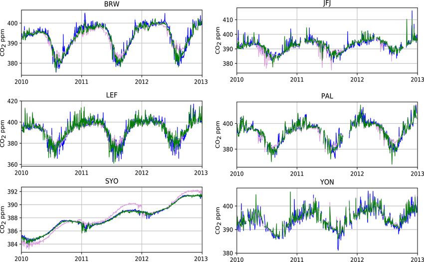
S. Maksyutov et al.: Technical note: A high-resolution inverse modelling technique for CO2 fluxes                             1247

sites (Manning et al., 2011). As a result, the global total of      geostrophic flow over flat terrain, as discussed by Ganshin et
regional emission estimates does not necessarily match the          al. (2012). It should be useful in the future to adapt this mod-
balance constrained by global mean concentration trends. A          elling framework to using reanalyses recently made available
global coupled Eulerian–Lagrangian model, such as Ganshin           at 0.25–0.3◦ resolution, even if the tests with higher resolu-
et al. (2012), has the potential to address both the objectives;    tion winds by Ware et al. (2019) did not show a large im-
that is, closing the global balance and operating at the range      provement over a lower resolution.
of scales from a single city (Lauvaux et al., 2016) to a large         The coupled transport model was derived from the
country or continental scale. Here we report the development        Global Eulerian–Lagrangian Coupled Atmospheric transport
of a high-resolution inverse modelling technique that is suit-      model (GELCA; Ganshin et al., 2012; Zhuravlev et al.,
able for application at a broad range of spatial scales. We ap-     2013; Shirai et al., 2017). To facilitate model application
plied it to the problem of estimating the distribution of CO2       in our iterative inversion algorithm, all the components of
fluxes over the globe that provides the best model fit to the       the model, i.e. the Eulerian model and the coupler, are in-
observations. In separate studies, the same inversion system        tegrated into one executable (online coupling), as described
was applied to the inverse modelling of methane emissions           in Belikov et al. (2016), while the original GELCA model
(Wang et al., 2019; Janardanan et al., 2020).                       implements Eulerian and Lagrangian components sequen-
   The objective of this study is to optimize the natural CO2       tially and then applies the coupler (offline coupling). The
fluxes in order to provide background CO2 concentration             changes in the current version with respect to the version
fields for estimating fossil CO2 emissions where the advan-         presented by Belikov et al. (2016) include an adjoint code
tage of the high-resolution approach is more evident. The pa-       derivation for model components, using the adjoint code
per is organized as follows: Sect. 1 provides an introduction,      compiler Tapenade (Hascoet and Pascual, 2013) instead of
Sect. 2 contains the transport model and its adjoint, Sect. 3       using the TAF (transformation of algorithms in Fortran) com-
introduces the prior fluxes, observational data set, and grid-      piler (Giering and Kaminski, 2003). Additionally, the in-
ded flux uncertainties, Sect. 4 gives the formulation of the in-    dexing and sorting algorithms for the transport matrix were
verse modelling problem and numerical solution, and Sect. 5         revised to allow efficient memory use for processing large
presents the simulation results and discussion, followed by         matrices of Lagrangian particle dispersion model (LPDM)-
the summary and conclusions.                                        driven responses to surface fluxes arising in the case of high-
                                                                    resolution surface fluxes and a large number of observa-
                                                                    tions, especially when using satellite data. A manually de-
2   The coupled tracer transport model, its adjoint, and            rived adjoint of the NIES-TM v08.1i is used, as in Belikov et
    the implementation                                              al. (2016), due to its computational efficiency. In the version
                                                                    of the model that includes the manually coded adjoint, only
For the simulation of the CO2 transport in the atmosphere,          the second-order van Leer algorithm (van Leer, 1977) is im-
we used the coupled Eulerian–Lagrangian model NIES-TM–              plemented, as opposed to the third-order algorithm typically
FLEXPART (defined as the National Institute for Environ-            used in forward models (Belikov et al., 2013).
mental Studies transport model coupled with the FLEXible
PARTicle dispersion model), which is a modified version
of the model described by Belikov et al. (2016). The cou-           3   Prior fluxes, flux uncertainties, and observations
pled transport model is computationally more efficient in
                                                                    Prior CO2 fluxes were prepared as a combination of monthly
comparison to the Eulerian model if both models are run
                                                                    varying fossil fuel emissions by the Open-Data Inven-
on the same spatial resolution. Belikov et al. (2016) con-
                                                                    tory for Anthropogenic Carbon dioxide (ODIAC), avail-
firmed that the coupled model with a Lagrangian model res-
                                                                    able at a global 30 arcsec resolution (e.g. Oda et al., 2018);
olution of 1◦ × ◦ performs similarly when coupled with Eu-
                                                                    ocean–atmosphere exchanges by the Ocean Tracer Transport
lerian model at either a 1.25◦ × 1.25◦ or 2.5◦ × 2.5◦ resolu-
                                                                    Model (OTTM) 4-D variational assimilation system, avail-
tion, and performance degradation was only seen when using
                                                                    able at a 1◦ resolution (Valsala and Maksyutov, 2010); daily
a 10◦ × 10◦ resolution Eulerian model. The coupled model
                                                                    CO2 emissions by biomass burning from the Global Fire As-
consists of NIES-TM v08.1i, with a horizontal resolution of
                                                                    similation System (GFAS) data set, provided by the Coper-
2.5◦ × 2.5◦ and 32 hybrid–isentropic vertical levels (Belikov
                                                                    nicus services at a 0.1◦ resolution (Kaiser et al., 2012); and
et al., 2013), and the FLEXPART model v.8.0 (Stohl et al.,
                                                                    the daily varying climatology of terrestrial biospheric CO2
2005), run in backward mode with a surface flux resolution
                                                                    exchange, simulated by the optimized Vegetation Integrative
of 0.1◦ × 0.1◦ . Both models use the Japan 25-year reanal-
                                                                    SImulator for Trace gases (VISIT) model (Ito, 2010; Saito et
ysis (JRA-25) and/or Japan Meteorological Agency (JMA)
                                                                    al., 2014). Figure 1 presents samples of the four prior flux
Climate Data Assimilation System (JCDAS) meteorology
                                                                    components (fossil, vegetation, biomass burning, and ocean)
(Onogi et al., 2007), with 40 vertical levels interpolated to a
                                                                    used in the forward simulation.
1.25◦ × 1.25◦ grid. The use of low-resolution wind fields for
high-resolution transport is better justified for cases of nearly

https://doi.org/10.5194/acp-21-1245-2021                                             Atmos. Chem. Phys., 21, 1245–1266, 2021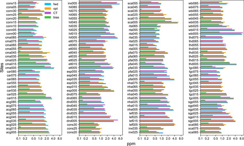
1248 S. Maksyutov et al.: Technical note: A high-resolution inverse modelling technique for CO2 fluxes
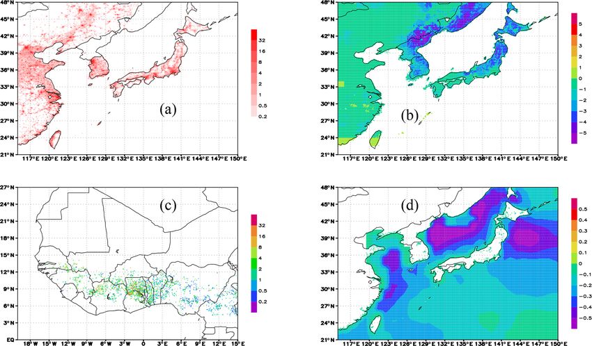
Figure 1. Examples of prior CO2 fluxes (units gC m−2 d−1 ). (a) Emissions from fossil fuel burning by ODIAC (January 2011). (b) Fluxes
from the terrestrial biosphere by the optimized VISIT model (day 160; 9 June 2011). (c) Emissions from biomass burning by GFAS in Africa
(10 January 2011). (d) Fluxes due to the ocean–atmosphere exchange by the OTTM assimilation model (January 2011).
3.1 Emissions from fossil fuel 3.2 Terrestrial biosphere fluxes
For the fossil fuel CO2 emissions (emissions due to fossil CO2 fluxes by the terrestrial biosphere at a resolution of 0.1◦
fuel combustion and cement manufacturing), we used the were constructed using a vegetation mosaic approach, com-
ODIAC data product (Oda and Maksyutov, 2011, 2015; Oda bining the vegetation map data by the Synergetic Land Cover
et al., 2018) at a 0.1◦ ×0.1◦ resolution on monthly basis. The Product (SYNMAP) data set (Jung et al., 2006), available
2016 version of the ODIAC data product (ODIAC2016; Oda at a 30 arcsec resolution, with terrestrial biospheric CO2 ex-
et al., 2018) is based on global and national emission esti- changes simulated by the optimized VISIT model (Saito et
mates and monthly estimates made by the Carbon Dioxide al., 2014) for each vegetation type in every 0.5◦ grid at a
Information Analysis Center (CDIAC; Boden et al., 2016; daily time step. The area fraction of each vegetation type is
Andres et al., 2011). For spatial disaggregation, it uses the derived from SYNMAP data for each 0.1◦ grid. The CO2 net
emission data for power plant emissions by the CARbon ecosystem exchange (NEE) fluxes on a 0.1◦ grid were pre-
Monitoring for Action (CARMA) database (Wheeler and pared by combining the vegetation-type-specific fluxes with
Ummel, 2008), while the rest of the national total emis- vegetation area fraction data on a 0.1◦ grid. By averaging the
sions on land were distributed using spatial patterns provided daily flux data for the period of 2000–2005, the flux clima-
by nighttime lights data collected by the Defence Meteoro- tology was derived for use in the recent years (after 2010)
logical Satellite Program (DMSP) satellites (Elvidge et al., when the VISIT model simulation based on JRA-25–JCDAS
1999). The ODIAC fluxes were aggregated to a 0.1◦ reso- reanalysis data was not available. Although the use of clima-
lution from the high-resolution ODIAC data (1 × 1 km). The tology in the place of original fluxes degrades the prior, the
ODIAC emission product is suitable for this kind of study be- posterior fluxes show significant departures from prior, thus
cause the global total emission is constrained by updated es- reducing the impact of missing the prior variations. The diur-
timates, while providing a high-resolution emission estimate. nal cycle was not resolved, as it requires one to also produce
Thus, it can be applied to carbon budget problems across dif- the gross primary production and ecosystem respiration. To
ferent scales. estimate the effect of excluding the diurnal cycle in the prior
fluxes for our selected time of sampling the observations,
Atmos. Chem. Phys., 21, 1245–1266, 2021 https://doi.org/10.5194/acp-21-1245-2021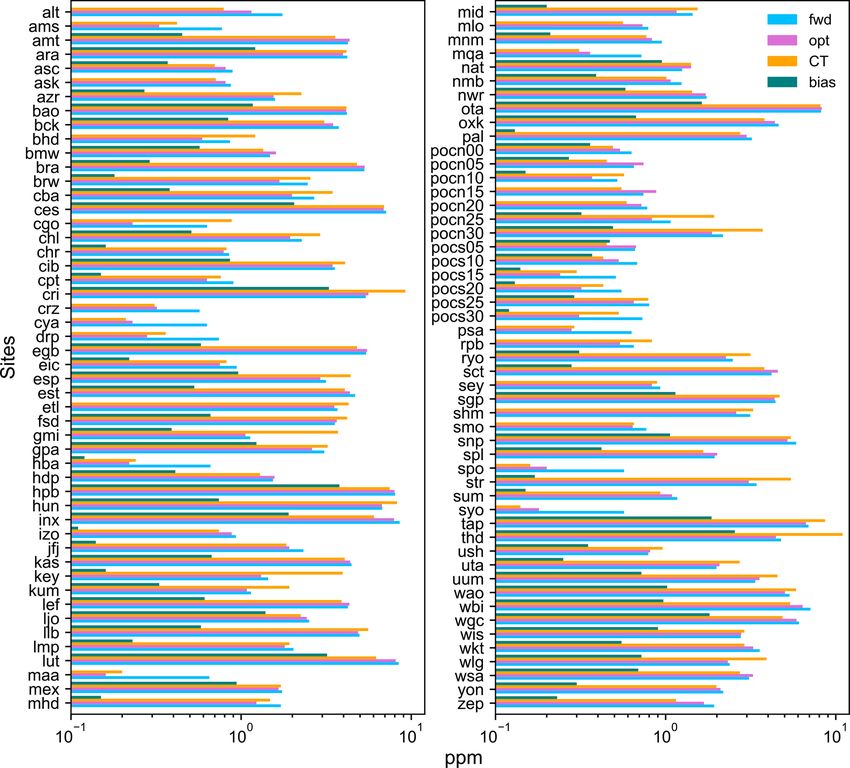
S. Maksyutov et al.: Technical note: A high-resolution inverse modelling technique for CO2 fluxes                         1249

we compared CO2 concentrations simulated with diurnally           3.5   Flux uncertainties for land and ocean
varying fluxes at an hourly time step with those made with
daily mean fluxes produced by the Simple Biosphere (SiB)          CO2 flux uncertainties are needed for both land and ocean re-
model for 2002–2003 (Denning et al, 1996), as used in the         gions. Climatological, monthly varying flux uncertainties for
Transcom continuous intercomparison (Law et al, 2008). The        land were set to 20 % of the MODIS gross primary produc-
results show that, for background monitoring sites, the differ-   tivity (GPP) product (MOD17A2), available on a 0.05◦ grid
ence is not significant (below 0.1 parts per million – ppm),      at a monthly resolution (Running et al., 2004). Oceanic flux
similar to the result by Denning et al. (1996). For continental   uncertainties were based on the sum of the standard deviation
sites, the difference between the two simulations was com-        of the OTTM assimilated flux from the climatology by Taka-
bined into four seasonal values, and the data for the season      hashi et al. (2009) and the monthly variance of the interan-
with the largest difference are shown in Fig. A1. Positive bias   nually varying OTTM fluxes (Valsala and Maksyutov, 2010),
by simulation with daily constant flux, with respect to diur-     with a minimum value of 0.02 gC m−2 d−1 , in the same way
nally varying fluxes, is of the order of 0.5 to 1 ppm, and it     as in the lower spatial resolution inverse model by Maksyu-
is larger during the middle of the growing season. Inclusion      tov et al. (2013). Oceanic flux uncertainties were first esti-
of the diurnally varying fluxes in the place of the daily mean    mated on a 1◦ ×1◦ resolution at a monthly time step and then
has the potential to change the seasonality of posterior fluxes   interpolated to a 0.1◦ × 0.1◦ grid, with the same procedure as
by inversion in a favourable direction, as there are regions      for the oceanic fluxes.
where flux seasonality is somewhat stronger than expected
(Sect. 5.2).                                                      3.6   Atmospheric CO2 observations

3.3   Emissions from biomass burning                              We used CO2 observation data distributed as the Ob-
                                                                  servation Package–CO2 (ObsPack–CO2 ) GLOBALVIEW-
Daily biomass burning CO2 emissions by the Global Fire As-        plus v2.1 (Cooperative Global Atmospheric Data Integra-
similation System (GFAS) data set rely on assimilating fire       tion Project, 2016). The data from the flask sites were used
radiative power (FRP) observations from the Moderate Res-         as an average concentration for a pair of flasks. Afternoon
olution Imaging Spectroradiometer (MODIS) instruments on          (15:00 to 16:00 LT – local time) average concentrations were
board the Terra and Aqua satellites (Kaiser et al., 2012). The    used for continuous observations over land and for remote
fire emissions at a 0.1◦ resolution are calculated from FRP       background observation sites. For the continuous moun-
with land-cover-specific conversion factors compiled from a       tain top observations, we used early morning observations
literature survey. The GFAS system adds corrections for ob-       (05:00 to 06:00 LT). The geographical local time was used,
servation gaps in the observations and filters spurious FRP       as defined by the universal coordinated time (UTC), with a
observations of volcanoes, gas flares, and other sources. The     longitude-dependent offset. The list of the observation loca-
fluxes are inputted to the model at the surface, which may        tions with the ObsPack site ID, site names, data providers,
lead to an underestimation of the injection height for strong     and data references appears in Table A1, accompanied by
burning events and the occasional overestimation of biomass       a site map in Fig. A2. The aircraft observational data col-
burning signals simulated at surface stations.                    lected by the NOAA aircraft programme at Briggsdale, Col-
                                                                  orado (CAR), Cape May, New Jersey (CMA), Dahlen, North
3.4   Oceanic exchange flux                                       Dakota (DND), Homer, Illinois (HIL), Portsmouth, New
                                                                  Hampshire (NHA), Poker Flats, Alaska (PFA), Rarotonga,
The air–sea CO2 flux component for the flux inversion used        Cook Islands (RTA), Charleston, South Carolina (SCA),
an optimized estimate of oceanic CO2 fluxes by Valsala and        Sinton, Texas (TGC; Sweeney et al., 2015), and also by
Maksyutov (2010). The data set was constructed with a vari-       the Comprehensive Observation Network for TRace gases
ational assimilation of the observed partial pressure of sur-     by AIrLiner (CONTRAIL) project over the western Pa-
face ocean CO2 (pCO2 ), available in Takahashi et al. (2017)      cific (CON; Machida et al., 2008) were grouped into averages
database, into the OTTM (Valsala et al., 2008), coupled with      for each 1 km altitude bin, with the altitude counted from sea
a simple one-component ecosystem model. The assimilation          level. Within the 1 km altitude range, the average value of
consists of a variational optimization method that minimizes      both concentration and the altitude was taken. Aircraft ob-
the model observation differences of the surface ocean dis-       servations were not assimilated, as they were only intended
solved inorganic carbon (DIC or pCO2 ) within the 2-month         for use in the validation of the results.
time window. The OTTM model fluxes produced on a 1◦ ×1◦
grid at monthly time step were interpolated to a 0.1◦ × 0.1◦
grid, taking into account the land fraction map derived from
the 1 km resolution MODIS land cover product.

https://doi.org/10.5194/acp-21-1245-2021                                          Atmos. Chem. Phys., 21, 1245–1266, 2021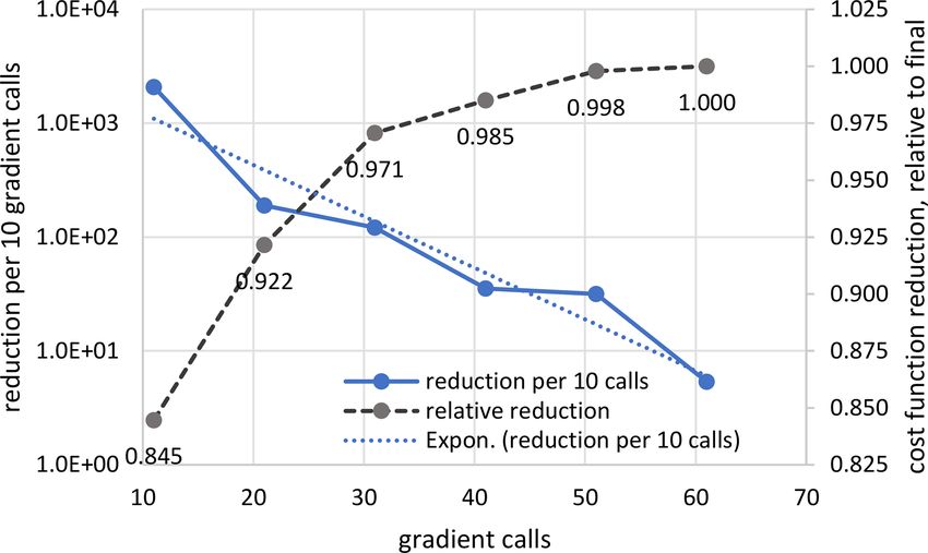
1250                     S. Maksyutov et al.: Technical note: A high-resolution inverse modelling technique for CO2 fluxes

4     Inverse modelling algorithm                                  fined as the norm of the difference between the NIES-TM–
                                                                   FLEXPART forward and adjoint modes estimated as (< y|H·
4.1    Flux optimization problem                                   x > − < HT · y|x >)/(< y|H · x >), was found to be of the
                                                                   order of 10−9 , while for the Lagrangian component based on
The inverse problem of atmospheric transport is formulated         the receptor sensitivity matrices prepared with FLEXPART,
by Enting (2002) as finding the surface fluxes that minimize       it is about 10−15 when calculated in double precision (same
the misfit between the transport model simulation y f + H ·        as in Belikov et al., 2016). The formulation of the minimiza-
(x p +x) and the vector of observations y, where y f is the for-   tion problem, as presented by Eq. (2), is convenient for the
ward simulation without the surface fluxes, x p is the known       derivation of the flux uncertainties, as it is possible to solve
prior flux, x is the unknown flux correction, and H represents     Eq. (3) via the truncated singular value decomposition (SVD)
the transport model. The equation y = y f +H·(x p +x) has to       and estimate the regional flux uncertainties based on the de-
be solved for the unknown flux correction x, and x is solved       rived singular vectors (Meirink et al., 2008). Alternatively,
for at the transport model grid scale (Kaminski et al., 2001).     as mentioned by Fisher and Courtier (1995), it is also pos-
By introducing the residual misfit vector r = y−(y f +H·x p ),     sible to use the flux increments derived at each iteration of
the problem can be formulated as minimizing a norm of dif-         the BFGS algorithm in the place of the singular vectors. Al-
ference (r − H · x) weighted by the data uncertainties. As         though we did not use SVD to construct the posterior covari-
the observation data alone are not sufficient to uniquely de-      ances in this study, we tested the solving of the optimization
fine the solution x, an additional regularization is required.     problem with SVD. We derived the SVD of AT A using a
By introducing additional constraints on the amplitude and         computer code by Wu and Simon (2000), which implements
smoothness of the solution, the inverse modelling problem is       an algorithm proposed by Lanczos (1950), and confirmed
formulated (Tarantola, 2005) as solving for the optimal value      that this approach yields practically the same solution as the
of the vector x at the minimum of a cost function J (x) as         one obtained with the BFGS algorithm. The Lanczos (1950)
follows:                                                           algorithm is a commonly used SVD technique, applied in the
       1                                  1                        case of a large, sparse matrix or a linear operator, when it is
J (x) = (H · x − r)T · R−1 · (H · x − r) + x T · B−1 · x, (1)      impractical to make direct use of the SVD of A. A truncated
       2                                  2
                                                                   SVD of A is given by the expression A ≈ U6VT , where 6 is
where x is the optimized flux, R is the covariance matrix          the diagonal matrix of n singular values, while U and V are
for observations, and B is the covariance matrix for surface       the matrices of left and right singular vectors. Variable sub-
fluxes. By introducing a decomposition of B as B = L · LT          stitutions, including the following:
(construction of matrix L explained in detail in Sect. 4.2) and
a variable substitution x = L · z, the second term in Eq. (1)      z = VT s, d = UT b,                                          (4)
is simplified. At the same time, by assuming that R can be
decomposed into R = σ T · σ , where σ is a vector of data un-      transform z into a space of singular vectors s and reduce
certainties, and introducing expressions b = σ −1 · (r − H · x)    Eq. (3) to (6 T 6 + I) · s = 6 T d, resulting in the following
and A = σ −1 · H · L, the new form of Eq. (1) is introduced as     solution:
follows:
                                                                   s = 6 T d/ 6 T 6 + I ,

                                                                                                                              (5)
          1
            (A · z − b)T (A · z − b) + zT · z .

J (z) =                                                     (2)
          2                                                        which is evaluated directly, as 6 is diagonal. In case of hav-
The solution minimizing J (z) can be obtained by forcing the       ing only n largest singular values, the elements of the so-
derivative ∂J (z)/∂z = AT (A · z − b) + z to be zero, which        lution s are given by si = λi di /(λ2i + 1) for all i ≤ n. Once
results in the following:                                          the solution (Eq. 5) is found, it is taken back to the space of
                                                                   the dimensional fluxes z by applying variable substitutions
 AT A + I · z = AT b.                                              (Eq. 4). For fluxes, we have x = L·z, z = VT s, and d = UT b;

                                                         (3)
                                                                   thus, the solution is provided by the following:
An optimal solution z at the minimum of the cost
function J (z) is found iteratively with the Broyden–                           6T
Fletcher–Goldfarb–Shanno (BFGS) algorithm (Broyden,                x = LV ·           · U T b.                                 (6)
                                                                              6T6 + I
1969; Nocedal, 1980), as implemented by Gilbert and
Lemarechal (1989). The method requires the ability to ac-          Another variant of the SVD approach may be more memory
curately estimate the cost function J (z) and its gradient         efficient in the case of a very large dimension of a flux vector.
AT (A · z − b) + z and has modest memory storage demands.          Then, applying SVD to AAT instead of AT A can save some
Given the solution z, the flux correction vector x is then         memory, as in a representer method (Bennett, 1992). It gives
found by reversing the variable substitution as x = L · z.         the same solution as the SVD of AT A and uses less interme-
  The convergence of the solution may be affected by the           diate memory storage when the dimension of the observation
accuracy of the adjoint. The result of the duality test, de-       vector y is lower compared to that of the flux vector x.

Atmos. Chem. Phys., 21, 1245–1266, 2021                                              https://doi.org/10.5194/acp-21-1245-2021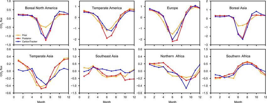
S. Maksyutov et al.: Technical note: A high-resolution inverse modelling technique for CO2 fluxes                            1251

   The forward and adjoint mode simulations with the trans-                  field and runs forward, with flux corrections up-
port model needed to implement the iterative optimization                    dated by the optimization algorithm at every iter-
are composed of several steps, as follows:                                   ation, to produce simulated concentrations. Correc-
                                                                             tions to the 3-D initial concentration field are not
 1. Running the Lagrangian model FLEXPART to produce                         estimated and, thus, not included in the control vec-
    the source–receptor sensitivity matrices. For each obser-                tor. Instead, the model is given a spin-up period of
    vation event, a backward transport simulation with the                   3 months before the target flux estimation period to
    FLEXPART model is implemented to produce the sur-                        adjust the simulated concentration to the observa-
    face flux footprints, at a 0.1◦ × 0.1◦ latitude–longitude                tions.
    resolution, and the 3-D concentration field footprint,
    taken at the end of the backward simulation run (ending               c. In the adjoint mode, the adjoint mode atmospheric
    at the coupling time of 00:00 Greenwich mean time –                      transport is simulated backward in time, starting
    GMT). The coupling time is set to be within 2 to 3 d be-                 from the vector of residuals to produce a gradient
    fore the observation event. The surface flux sensitivity                 of the cost function (defined as Eq. 1) with respect
    data are recorded in the unit of ppm (gC m−2 d−1 )−1 .                   to the surface fluxes. Given the gradient, the opti-
    The flux footprints are saved at a daily or hourly time                  mization algorithm provides the new flux correc-
    step, depending on available surface fluxes.                             tions field. For convenience, the transport model
                                                                             and its adjoint are implemented as procedures suit-
 2. Running the coupled transport model forward, which in-                   able for direct communication mode.
    cludes the following:
                                                                    Step 1 is carried out in the same way as in other versions of
      a. Running the 3-D Eulerian model NIES-TM from                the coupled transport model (Zhuravlev et al., 2013; Shirai
         the 3-D initial concentration field, with the pre-         et al., 2017). In steps 2 and 3, the procedure of running the
         scribed surface fluxes. This includes sampling the         forward and adjoint model is organized differently. At the be-
         3-D field at model coupling times for each obser-          ginning of the transport model runs, all the data prepared by
         vation, according to 3-D concentration field foot-         the Lagrangian model are stored in the computer memory in
         prints calculated at the first step by FLEXPART.           order to save on the time required for reading and re-sorting
         NIES-TM reads the same 0.1◦ fluxes as the La-              the data at each iteration. The fraction of the CPU time spent
         grangian transport model and remaps them onto its          on running the Eulerian component of the coupled transport
         2.5◦ × 2.5◦ grid before including them in the sim-         model is 82 %, with 1 % used on the Lagrangian component
         ulation. For each observation event, the fluxes used       and 17 % used for covariance.
         in Eulerian and Lagrangian components are sepa-               To create the initial concentration field, we used a 3-D
         rated by the coupling time, so that there is no double     snapshot of the CO2 concentration for the same day from
         counting of fluxes for the same date in the coupled        a simulation of the previous year, which is already optimized
         model simulation.                                          (usually 1 October or 1 January). When such a simulation
      b. Using the two-dimensional (2-D) surface flux foot-         was not available, we took a snapshot from an available year
         prints prepared with the Lagrangian model to cal-          and corrected it globally for the concentration difference be-
         culate the surface flux contribution to the simulated      tween these years, using the NOAA monthly mean data for
         concentrations for the last 3 d.                           the South Pole as representative for the global mean concen-
      c. Combining the concentration contributions pro-             tration. When the optimized fields are not available, the out-
         duced by Eulerian (a) and Lagrangian (b) compo-            put of the multiyear spin-up simulation is used, with the same
         nents to give the total simulated concentration.           adjustment to the South Pole observations.

 3. In the inverse modelling, the transport model is run in         4.2   Implementation of covariance matrices L and B
    the following three modes:
                                                                    We optimized surface flux fields separately for two sets of
      a. The forward model is first run with prescribed prior       fluxes in every grid globally, for land and ocean regions, fol-
         fluxes, starting from the 3-D initial CO2 concentra-       lowing the approaches by Meirink et al. (2008) and Basu
         tion field, to calculate the residual misfit (difference   et al. (2013), who suggested optimizing for global surface
         between the observation and the model simulation).         flux fields separately for each optimized flux category. Sep-
      b. At the inverse modelling/optimization step, only           arating the total flux into independent flux categories, each
         the flux corrections are propagated in the for-            with its own flux uncertainty pattern, results in using ho-
         ward model runs, which are optimized to minimize           mogenous spatial covariance matrices, significantly simpli-
         the observation–model misfit. The prescribed prior         fying the coding of the matrix B. The matrix B can be given
         fluxes are not used (switched off) at this step. The       as the product of a diagonal matrix of flux uncertainties and a
         model starts from a zero 3-D initial concentration         matrix with 1.0 as diagonal elements, while non-diagonal el-

https://doi.org/10.5194/acp-21-1245-2021                                             Atmos. Chem. Phys., 21, 1245–1266, 2021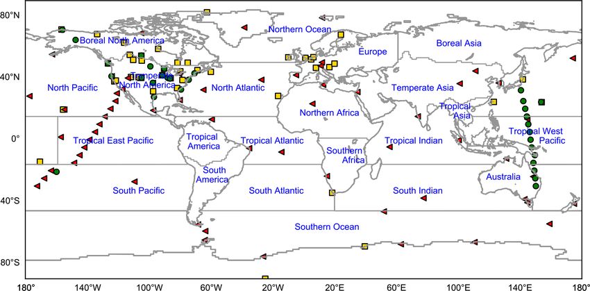
1252                     S. Maksyutov et al.: Technical note: A high-resolution inverse modelling technique for CO2 fluxes

ements are exponentially declining with the squared distance        where D is the diffusivity. The solution of Eq. (8) is given by
between grid points (Meirink et al., 2008). In practice, an                        Rl
extra scaling of the uncertainty is needed to balance the con-      g̃(λ) = √ 1 2 exp(− 12 (λ−λ0 )2 /p2 )g(λ0 )dλ0 , where p 2 =
                                                                              2πp −l
straint on fluxes with the data uncertainty, which also impacts     2D1t, g(λ) is the initial distribution, and 1t is the time step
the regional flux uncertainties. Several empirical methods are      (Crank, 1975). Based on this equivalence, instead of multi-
in use, where the tuning parameters are a horizontal scale          plying a vector by the covariance matrix, we solve the dis-
(Meirink et al., 2008) and an uncertainty multiplier (Cheval-       crete form of Eq. (8) by the backward-in-time, central-in-
lier et al., 2005; Rödenbeck, 2005). In our B matrix design,        space implicit method.
we follow Meirink et al. (2008) in representing B matrix as            Applying the diffusion operator for the covariance matrix
the multiple of the non-dimensional covariance matrix C and         helps to achieve the spatial homogeneity between polar and
the diagonal matrix of the flux uncertainty D as B = DT ·C·D.       equatorial regions, as diffusion produces a theoretically uni-
C matrix is commonly implemented as a band matrix, with             form effect on flux fields – regardless of the polar singularity.
non-diagonal elements declining as ∼ exp(−x 2 /l 2 ), with the      The diffusion operator works as a low-pass filter, selectively
distance x between the grid cells as in 2-D spline algorithms       suppressing all the wavelengths shorter than the covariance
(Wahba and Wendelberger, 1980). Multiplication by the ma-           length scale. As we need to construct the covariance matrix B
trix C becomes computationally costly at a high spatial res-        in the form B = L·LT , we choose to construct L first and then
olution in cases where the correlation distance l is much           derive its transpose LT . The factorization of L is given by
larger than the size of the model grid. The correlation dis-        L = uF · (Lxy ⊗ Lt ) · m, where Lt is the 1-D covariance ma-
tance used here is 500 km for land and ocean and 2 weeks            trix for the time dimension, and ⊗ is a Kronecker product.
in time. The rationale of applying a correlation distance of        We approximate the 2-D covariance Lxy by splitting it into
500 km in the case of a regional inversion over the continen-       two dimensions, namely latitude and longitude as in Chua
tal USA with a model grid size of 40 km was discussed by            and Bennett (2001), and apply several iterations of this pro-
Schuh et al. (2010). In that case, the use of an implicit diffu-    cess. The horizontal covariance Lxy is implemented in N = 3
sion with a directional splitting to approximate the Gaussian       iterations of 1-D diffusion so that Lxy = (Lx ⊗ Ly )N , where
shape appears to be computationally more efficient than the         Lx and Ly are the covariance operators for longitude and lat-
direct application of the Gaussian-shaped smoothing func-           itude directions, respectively, while uF is the diagonal matrix
tion, as the number of floating-point operations per grid point     of flux uncertainty for each grid cell and each flux category
does not grow with the ratio of the correlation distance l to       (land and ocean), and m is the diagonal matrix of a map fac-
the grid size. The covariance matrix based on the diffusion         tor, which is introduced to scale the contributions to the cost
operator is popular in many ocean data assimilation systems,        function by model grid area, with diagonal elements given by
as it is a convenient way to deal with coastlines (e.g. Derber      m = cos−1/2 θ (where θ is latitude).
and Rosati, 1989; Weaver and Courtier, 2001).                          This design of the covariance operator helps to preserve
   The idea of using the solution of the diffusion equation in-     the high-resolution structure of the resultant flux corrections,
stead of multiplying a vector by the covariance matrix can          given by x = L · z = uF · (Lxy ⊗ Lt ) · m · z, as it can be fac-
be presented briefly in a 1-D case. Consider a discrete prob-       tored into a multiple of uncertainty uF and a scaling factor
lem of multiplying a vector representing a function g(λ) on a       S = (Lxy ⊗ Lt ) · m · z as x = uF · S. While the scaling fac-
grid with spacing 1λ by a symmetric matrix which has diag-          tor S is smoothed with a covariance length of 500 km, the
onal elements equal to one, and non-diagonal ones declining         original structure of the spatial heterogeneity of surface flux
as exp(− 12 (i1λ)2 /d 2 ), with a distance of i points from the     uncertainty uF is still preserved at the original high resolution
diagonal, where d is covariance length. Its continuous ana-         in the optimized flux corrections x.
logue is an application of a Gaussian-shaped smoother in the           The adjoint operators LTx and LTy are derived by apply-
form G(λ, λ0 ) = exp(− 21 (λ − λ0 )2 /d 2 ) to a function g(λ) as   ing the adjoint code compiler Tapenade (Hascoet and Pas-
follows:                                                            cual, 2013) to the Fortran code of modules that approxi-
          Zl                                                        mate the operators Lx and Ly by implicit diffusion. Lt and
                                                                    its transpose LTt are of lower dimensions and are designed,

                    1      0 2 2
g̃(λ) =        exp − (λ − λ ) /d g(λ0 )dλ0 ,                 (7)
                    2                                               as in Meirink et al. (2008), by deriving the square root of
          −l                                                        the Gaussian-shaped time covariance matrix with direct SVD
where the smoothing window size l should be several times           (Press et al., 1992).
larger than d. The expression in Eq. (7) looks exactly like the        A notable merit of the algorithm is that it minimizes the
solution of a 1-D diffusion equation, as follows:                   use of the computer’s memory, avoiding allocations of the
                                                                    memory space that are larger than several times the dimen-
∂g    ∂ 2g                                                          sion of the observation and flux vectors, making it suitable
   − D 2 = 0,                                                (8)    for ingesting large amounts of surface and space-based ob-
∂t    ∂λ
                                                                    servations. It should be mentioned that the computer memory

Atmos. Chem. Phys., 21, 1245–1266, 2021                                                https://doi.org/10.5194/acp-21-1245-2021
S. Maksyutov et al.: Technical note: A high-resolution inverse modelling technique for CO2 fluxes 1253
demand for accommodating the surface flux sensitivity ma- 5 Results and discussion
trices for massive space-based observations can be a limiting
factor, as discussed by Miller et al. (2020). 5.1 Analysis of the posterior model fit to the
observations
4.3 Inversion set-up
We compared the results of the forward simulation with prior
The combination of the coupled transport model NIES-TM– and optimized fluxes with the processed observations for
FLEXPART (as described in Sect. 2) with the variational ground observation sites, as shown in Table A1, and air-
optimization algorithm (Sect. 4.1 and 4.2) constitutes the borne vertical profiles were used for an independent valida-
inverse modelling system NIES-TM–FLEXPART-VAR (NT- tion (Table A2). Figure 2 shows the observations with for-
FVAR or NIES-TM–FLEXPART-variational). We tested the ward (prior) and optimized simulations at Barrow (BRW),
inversion algorithm presented in previous sections with the Jungfraujoch (JFJ), Wisconsin (LEF), Pallas (PAL), Yonagu-
problem of finding the best fit to the CO2 observations pro- nijima (YON), and Syowa (SYO). The optimization yielded
vided by the ObsPack data set by optimizing the corrections improved seasonal variations in the simulated concentration,
to the land and ocean fluxes. By design, our inverse mod- including the phase and the amplitude at most sites. At SYO,
elling system produced smoothed fields of scaling factors we found synoptic scale variations with an amplitude of the
that are multiplied by the fine-resolution flux uncertainty order of few tenths of a part per million that were, to a
fields to give flux corrections. We derived the surface CO2 large extent, captured by the model. Plots for BRW and JFJ
flux corrections at a 0.1◦ resolution and biweekly time step. show the ability of the inversion to correct the seasonal cycle,
Our purpose is to demonstrate that we can optimize fluxes while the difference between model and observations in the
to improve the fit to the observations, using an iterative Southern Hemisphere (SYO) is contributed by the interan-
optimization procedure based on a high-resolution coupled nual variations in the carbon cycle. The model–observation
transport model and its adjoint. Our report is limited to the mismatch (RMSE) for surface sites included in the ObsPack
technical development towards achieving the capability of is presented in Fig. 3 for forward and optimized simulation
estimating anthropogenic CO2 emissions based on atmo- and mean bias for optimized data. The model was able to
spheric observations, and we do not elaborate on the impact reduce the model to observation mismatch for most back-
of simulating the tracer transport at a high resolution on ground sites where the seasonal cycle is affected mostly by
the quality of the optimized natural fluxes, which requires natural terrestrial and oceanic fluxes, while the average re-
an additional study. The flux optimization was applied to a duction in the mismatch from forward to optimized simula-
short time window of 18 months for each optimized year, tion is 14 %, which is defined as the mean ratio of the op-
and the simulation starts on 1 October, 3 months ahead of timized mismatch to the forward mismatch taken for each
the target year. A spin-up period of 3 months is given to site. The reason for the relatively small reduction is the addi-
let the inversion adjust the modelled concentration to the tion of climatological flux corrections to the prior simulation,
observations so that a balance is achieved between fluxes, estimated by inverse modelling of 2 years of data, namely
concentrations, and concentration trends. The simulation 2009 and 2010. As a result, the inversion starts from the
is continued until reaching the limit of 45 cost function initial flux distributions already adjusted to fit the seasonal
gradient calls, and by that time, the M1QN3 procedure cycle of the observed concentration. The correction for the
by Gilbert and Lamarechal (1989) is able to complete difference in the global concentration trend between years is
30 iterations. Figure A3 presents the cost function reduction not made; thus, there are visible differences between prior
in the case of optimizing fluxes for 2011 and completing and optimized simulations in the southern hemispheric back-
61 gradient calls. The cost function reduction declines ground sites. At most of the Antarctic sites, the mean poste-
nearly exponentially, by almost 3 times, for each 10 gradient rior (after optimization) mismatch (reported as RMSE) is of
calls completed. The relative improvement between 41 and the order of 0.2 ppm. Over the land, closer to anthropogenic
61 gradient calls is 1.5 % of the total reduction from the first sources, there is a less relative reduction in the mismatch on
to the 61 gradient calls. We optimized fluxes for 3 years an annual mean scale. One of the reasons for seeing little
from 2010 to 2012 and analysed the simulated concentration improvement is that fossil CO2 emissions are kept fixed and
fit at the observation sites. The average root mean squared only the natural fluxes are optimized (while the strong sig-
misfits (RMSE) between the optimized concentrations and nal from fossil emission is not affected by flux corrections).
the observations are compared with a forward simulation Another possible contributor to the large mismatch over land
with prior fluxes and optimized simulation. For evaluation, is the neglect of the diurnal cycle, under the assumption of
we used statistics of the optimized simulations by the op- using only observations at well-mixed conditions, and also
erational NOAA’s CarbonTracker inverse modelling system the limited ability of the low-resolution reanalysis data set to
(ObsPack_co2_1_CARBONTRACKER_CT2017_2018-05- capture frontal processes in the extratropical continental at-
02; Peters et al., 2007). mosphere, as discussed by Parazzoo et al. (2011). The mean
mismatch was reduced from 2.60 to 2.42 ppm by the flux op-
https://doi.org/10.5194/acp-21-1245-2021 Atmos. Chem. Phys., 21, 1245–1266, 20211254 S. Maksyutov et al.: Technical note: A high-resolution inverse modelling technique for CO2 fluxes timization, while the mean mismatch to the uncertainty ratio Tracker shows a better fit at most of the altitude ranges, decreases after optimization by 19 % from 0.94 to 0.78. The except for the lowest 1 km where the results shown by the mean correlation between modelled and observed data im- two systems were similar. Concurrently, the mean correla- proves from r 2 = 0.43 (r 2 – coefficient of determination) for tion between modelled and observed data did not improve the simulation driven by prior fluxes to r 2 = 0.59 for the op- from the prior (r 2 = 0.70) to the optimized simulation (r 2 = timized simulation. To remove the effect of the interannual 0.63), while the mean RMSE declined a little from 1.86 to CO2 growth on CO2 variabilities, the mean growth trend was 1.85 ppm. The comparison to CarbonTracker (CT 2017), subtracted from the data before estimating the r 2 . with a mean RMSE of 1.53 ppm, suggests that the free tro- Figure 3 also shows, for the purpose of comparison, the pospheric performance of our system can be improved by statistics of the average misfit for the optimized simulation implementing a more detailed vertical mixing processes in by CarbonTracker for the same period and same monitor- the Lagrangian and Eulerian component models. ing stations. The comparison is useful for understanding the strengths and weaknesses of the inversion system pre- 5.2 Comparison of prior and posterior fluxes sented here. Over the background monitoring sites, the high- resolution model does not show any advantage over Carbon- As mentioned in Sect. 4.2, the flux corrections estimated by Tracker in terms of the fit between the optimized model sim- the inverse model showed fine-scale features, despite using ulation and observations, which may indicate a better perfor- large covariance lengths, because those were made of the mance by the Eulerian model, TM5, used in CarbonTracker. high-resolution data uncertainty multiplied by the smooth On the other hand, several sites where the high-resolution fields of scaling factor and estimated separately for each of model shows better fits to observations over CarbonTracker the optimized flux categories, namely land biosphere and are located inland or near the coast, closer to anthropogenic ocean. Examples of the flux corrections and posterior fluxes and biogenic sources. A smaller misfit was achieved by (excluding fossil emissions) are presented in Fig. 5. The flux the high-resolution model at Key Biscayne (KEY), Bar- corrections and fluxes are shown in Fig. 5 for 1 month (Au- ing Head (BHD), Mariana Islands (GMI), and Cape Ku- gust 2011) as an illustration, and they are not representative mukahi (KUM), among others, which can be attributed to of a seasonal or climatological mean. The sign of the flux coastal/island locations, while there is little or no advan- corrections changed from positive (source) in the eastern side tage at mountain sites like Mauna Loa (MLO) or Jungfrau- (continental China) to negative (sink) over the Russian coast joch (JFJ). This result may be influenced by differences in the and Japanese islands, while the posterior fluxes appeared as model physics between NIES-TM–FLEXPART and TM5 in a terrestrial sink all over the area. The flux adjustment was the lower troposphere, near the top of the boundary layer, and driven by the fit to nearby observations made over South Ko- in shallow cumuli. The mismatch (RMSE) between our op- rea and Japan. timized model and observations for the 102 sites used in the To illustrate the change in fluxes from prior to posterior inversion is only 4 % lower on average than that by Carbon- estimates by the inversion at the scale of large aggregated re- Tracker. It is not yet clear if there is a systematic advantage of gions, the monthly mean fluxes (excluding fossil emissions) one or the other system in any particular site category, other averaged for 3 years (2010–2012) are plotted in Fig. 6 for than for coastal/island sites mentioned above. For the average eight selected Transcom regions (as defined by Gurney et misfit comparison, all data, both assimilated and not assimi- al., 2002; see the map in Fig. A2). The plots include prior, lated, are included for sites shown in Fig. 3. The results for optimized, and, for reference, optimized fluxes by Carbon- Cape Grim (CGO) were not counted due to the use of differ- Tracker (CT 2017). For some regions, the posterior is close ent data sets, as our system used only the NOAA flask data, to the prior, which is often the case when there are too few which underwent background selection (by wind direction) observations in the region to drive the corrections to prior at the time of sampling. fluxes. Boreal North America (region 1), temperate North As an independent validation, a comparison of the unop- America (region 2), and Europe (region 11) are better con- timized and optimized simulation to the vertical profile data strained by observations, while Northern Africa (region 5), is shown in Fig. 4. For each vertical profile site, the observa- Southern Africa (region 6), temperate Asia (region 8), trop- tions were grouped by altitude, at a 1 km interval. The alti- ical Asia (region 9), and boreal Asia (region 7) are less tude code (e.g. 005, 015, 025, 035, . . . ) to be added to the site constrained. The optimized flux is similar to the prior for identifier was constructed as the altitude of the midlevel mul- Africa (regions 5 and 6), tropical Asia (region 9), and tem- tiplied by 10. The observations at PFA (Poker Flat, Alaska) perate Asia (region 8), while there is a substantial adjustment between the surface and 1 km were grouped as PFA005 (mid- for boreal Asia (region 7), which seems to be adjusted to fit altitude 0.5 km), while those in the 5 to 6 km range were the observations outside the region. For both boreal regions, designated as PFA055 (mid-altitude 5.5 km). As for the op- the prior flux seasonality appears weaker than in both poste- timized surface data in Fig. 3, we show the RMSE for for- rior and CarbonTracker fluxes, which could indicate a prob- ward simulation with prior fluxes, optimized simulation, and lem with vegetation-type mapping in a higher resolution ver- CarbonTracker and mean bias for optimized data. Carbon- sion of the prior flux model. For regions 1, 6, 7, and 11, the Atmos. Chem. Phys., 21, 1245–1266, 2021 https://doi.org/10.5194/acp-21-1245-2021
S. Maksyutov et al.: Technical note: A high-resolution inverse modelling technique for CO2 fluxes                             1255

Figure 2. Time series of simulated and observed concentrations (blue – observed; plum – forward (unoptimized); green – optimized) at
Barrow (BRW), Jungfraujoch (JFJ), Wisconsin (LEF), Pallas (PAL), Syowa (SYO), and Yonagunijima (YON).

Figure 3. Root mean square difference between model and observations and absolute bias in 2010–2012 for (surface) sites included in
inversion (blue – prior; pink – optimized; orange – CT 2017; green – absolute value of mean difference (bias) for optimized).

https://doi.org/10.5194/acp-21-1245-2021                                             Atmos. Chem. Phys., 21, 1245–1266, 2021
1256 S. Maksyutov et al.: Technical note: A high-resolution inverse modelling technique for CO2 fluxes
Figure 4. Root mean square difference between model and observations and absolute bias in 2010–2012 for aircraft sites not included in
inversion (blue – prior; orange – optimized; magenta – CT 2017; green – absolute value of mean difference (bias) for optimized).
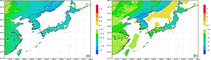
Figure 5. Optimized flux correction (a) and posterior flux (b) maps for August 2011 (units gC m−2 d−1 ; fossil emissions excluded).
corrected fluxes are closer to CarbonTracker, and for tem- 6 Summary and conclusions
perate North America, temperate Asia, and Northern Africa,
the amplitude of flux seasonality is estimated to be stronger,
which can be caused by stronger vertical/horizontal mixing A grid-based CO2 flux inversion system that is suitable for
in the transport model as compared to the transport in Car- the inverse estimation of the surface fluxes at a biweekly time
bonTracker. A more detailed comparison with other inverse step and a 0.1◦ spatial resolution was developed. To imple-
model results and independent estimates (e.g. by Jung et al., ment the high-resolution simulation capability, several devel-
2020) should be made after improving the inversion set-up, opments were completed. High-resolution prior fluxes were
notably by improving the transport model meteorology, sea- prepared for the following three surface flux categories: fos-
sonality, and diurnal cycle in prior fluxes and the seasonality sil emissions by the ODIAC data set were based on the point
in prior flux uncertainties. source database and night lights, biomass burning emis-
sions (GFAS) were based on MODIS observations of fire
radiative power, and biosphere exchange was based on the
Atmos. Chem. Phys., 21, 1245–1266, 2021 https://doi.org/10.5194/acp-21-1245-2021You can also read