DEEPMIP: MODEL INTERCOMPARISON OF EARLY EOCENE CLIMATIC OPTIMUM (EECO) LARGE-SCALE CLIMATE FEATURES AND COMPARISON WITH PROXY DATA - OCEANREP
←
→
Page content transcription
If your browser does not render page correctly, please read the page content below
Clim. Past, 17, 203–227, 2021
https://doi.org/10.5194/cp-17-203-2021
© Author(s) 2021. This work is distributed under
the Creative Commons Attribution 4.0 License.

DeepMIP: model intercomparison of early Eocene climatic
optimum (EECO) large-scale climate features and
comparison with proxy data
Daniel J. Lunt1 , Fran Bragg1 , Wing-Le Chan2 , David K. Hutchinson3 , Jean-Baptiste Ladant4 , Polina Morozova5 ,
Igor Niezgodzki6,7 , Sebastian Steinig1 , Zhongshi Zhang8,9 , Jiang Zhu4 , Ayako Abe-Ouchi2 , Eleni Anagnostou10 ,
Agatha M. de Boer3 , Helen K. Coxall3 , Yannick Donnadieu11 , Gavin Foster12 , Gordon N. Inglis12 , Gregor Knorr6 ,
Petra M. Langebroek8 , Caroline H. Lear13 , Gerrit Lohmann6 , Christopher J. Poulsen4 , Pierre Sepulchre14 ,
Jessica E. Tierney15 , Paul J. Valdes1 , Evgeny M. Volodin16 , Tom Dunkley Jones17 , Christopher J. Hollis18 ,
Matthew Huber19 , and Bette L. Otto-Bliesner20
1 School  of Geographical Sciences, University of Bristol, Bristol, UK
2 Atmosphere    and Ocean Research Institute, University of Tokyo, Tokyo, Japan
3 Department of Geological Sciences, Stockholm University, Stockholm, Sweden
4 Department of Earth and Environmental Science, University of Michigan, Ann Arbor, USA
5 Institute of Geography, Russian Academy of Sciences, Moscow, Russia
6 Alfred Wegener Institute, Helmholtz Centre for Polar and Marine Research, Bremerhaven, Germany
7 ING PAN – Institute of Geological Sciences, Polish Academy of Sciences, Research Center in Kraków,

Biogeosystem Modelling Group, Kraków, Poland
8 NORCE Norwegian Research Centre, Bjerknes Centre for Climate Research, Bergen, Norway
9 Department of Atmospheric Science, School of Environmental Studies, China University of Geosciences, Wuhan, China
10 GEOMAR Helmholtz Centre for Ocean Research Kiel, Kiel, Germany
11 Aix Marseille Univ, CNRS, IRD, INRA, Coll France, CEREGE, Aix-en-Provence, France
12 School of Ocean and Earth Science, National Oceanography Centre Southampton,

University of Southampton, Southampton, UK
13 School of Earth and Environmental Sciences, Cardiff University, Cardiff, UK
14 Laboratoire des Sciences du Climat et de l’Environnement, LSCE/IPSL, CEA-CNRS-UVSQ,

Université Paris-Saclay, Gif-sur-Yvette, France
15 Department of Geosciences, University of Arizona, Tucson, USA
16 Marchuk Institute of Numerical Mathematics, Russian Academy of Sciences, Moscow, Russia
17 School of Geography, Earth and Environmental Sciences, Birmingham University, Birmingham, UK
18 Surface Geosciences, GNS Science, Lower Hutt, New Zealand
19 Department of Earth, Atmospheric, and Planetary Sciences, Purdue University, West Lafayette, USA
20 Climate and Global Dynamics Laboratory, National Center for Atmospheric Research, Boulder, USA

Correspondence: Daniel J. Lunt (d.j.lunt@bristol.ac.uk)

Received: 10 December 2019 – Discussion started: 2 January 2020
Revised: 23 October 2020 – Accepted: 1 November 2020 – Published: 15 January 2021

Published by Copernicus Publications on behalf of the European Geosciences Union.
204                                                                     D. J. Lunt et al.: DeepMIP model–data comparison

Abstract. We present results from an ensemble of eight           cially relevant because they share characteristics with pos-
climate models, each of which has carried out simulations        sible future climates (Burke et al., 2018). In this context,
of the early Eocene climate optimum (EECO, ∼ 50 million          there has been a community focus on the Pliocene (∼ 3–
years ago). These simulations have been carried out in the       5 million years ago; Haywood et al., 2013) and Eocene
framework of the Deep-Time Model Intercomparison Project         (∼ 50 million years ago; Lunt et al., 2012), which pro-
(DeepMIP; http://www.deepmip.org, last access: 10 January        vide natural examples of past worlds with high CO2 con-
2021); thus, all models have been configured with the same       centrations of ∼ 300–400 ppmv and ∼ 1200–2500 ppmv re-
paleogeographic and vegetation boundary conditions. The          spectively. In this paper, we focus on the Eocene, present-
results indicate that these non-CO2 boundary conditions con-     ing model results that have recently been produced in the
tribute between 3 and 5 ◦ C to Eocene warmth. Compared           framework of the Deep-Time Model Intercomparison Project
with results from previous studies, the DeepMIP simulations      (DeepMIP; http://www.deepmip.org; Lunt et al., 2017; Hol-
generally show a reduced spread of the global mean surface       lis et al., 2019) and the associated model–data comparisons.
temperature response across the ensemble for a given atmo-       Given the similarity of Eocene CO2 concentrations and cli-
spheric CO2 concentration as well as an increased climate        mate to those that are attained under high-growth and low-
sensitivity on average. An energy balance analysis of the        mitigation future scenarios considered by the IPCC (Burke
model ensemble indicates that global mean warming in the         et al., 2018), the Eocene provides a potential test bed for
Eocene compared with the preindustrial period mostly arises      state-of-the-art climate model predictions of the future.
from decreases in emissivity due to the elevated CO2 con-           Eocene modelling and model–data comparisons have a
centration (and associated water vapour and long-wave cloud      long history (e.g. Barron, 1987; Sloan and Barron, 1992).
feedbacks), whereas the reduction in the Eocene in terms of      More recently, Lunt et al. (2012) carried out a synthesis of
the meridional temperature gradient is primarily due to emis-    a group of models that had all conducted Eocene simulations
sivity and albedo changes owing to the non-CO2 boundary          (Lunt et al., 2010b; Heinemann et al., 2009; Winguth et al.,
conditions (i.e. the removal of the Antarctic ice sheet and      2010; Huber and Caballero, 2011; Roberts et al., 2009), with
changes in vegetation). Three of the models (the Community       a focus on surface temperatures. Subsequent work also ex-
Earth System Model, CESM; the Geophysical Fluid Dynam-           plored the precipitation in the simulations (Carmichael et al.,
ics Laboratory, GFDL, model; and the Norwegian Earth Sys-        2016) and the implications for ice sheet growth (Gasson
tem Model, NorESM) show results that are consistent with         et al., 2014). This was an “ensemble of opportunity” in that
the proxies in terms of the global mean temperature, merid-      the model simulations were carried out independently, using
ional SST gradient, and CO2 , without prescribing changes        a variety of paleogeographic and vegetation boundary condi-
to model parameters. In addition, many of the models agree       tions, under a range of different CO2 concentrations. A proxy
well with the first-order spatial patterns in the SST prox-      data synthesis was also produced as part of the Lunt et al.
ies. However, at a more regional scale, the models lack skill.   (2012) study, consisting of sea surface temperatures (SSTs)
In particular, the modelled anomalies are substantially lower    and a previously compiled continental temperature dataset
than those indicated by the proxies in the southwest Pacific;    (Huber and Caballero, 2011). This model–data comparison
here, modelled continental surface air temperature anoma-        showed that (a) there was a wide spread in the global mean
lies are more consistent with surface air temperature proxies,   temperature response across the models for a given CO2 con-
implying a possible inconsistency between marine and ter-        centration – e.g. at CO2 concentrations 4 times (× 4) those of
restrial temperatures in either the proxies or models in this    the preindustrial simulation, the range in the modelled global
region. Our aim is that the documentation of the large-scale     mean continental near-surface air temperature was 5.8 ◦ C;
features and model–data comparison presented herein will         (b) given CO2 concentrations 16 times those of the prein-
pave the way to further studies that explore aspects of the      dustrial simulation (× 16), the Community Climate System
model simulations in more detail, for example the ocean cir-     Model (CCSM3) model was able to reproduce the mean cli-
culation, hydrological cycle, and modes of variability, and      mate and meridional temperature gradient indicated by the
encourage sensitivity studies to aspects such as paleogeogra-    proxies; (c) the Hadley Centre Climate Model (HadCM3)
phy, orbital configuration, and aerosols.                        had relatively weak polar amplification compared with the
                                                                 other models; (d) the climate sensitivity across the models
                                                                 was fairly similar, but HadCM3 had a notable non-linearity
1   Introduction                                                 in sensitivity, in contrast to CCSM3; and (e) interpreting
                                                                 middle- and high-latitude proxy SSTs as representing sum-
Paleoclimate model–data comparisons allow us to (1) assess       mer temperatures brought the modelled temperatures closer
confidence in the results from model sensitivity studies that    to those indicated by the proxies.
explore the mechanisms that drove past climate change and           At that time, due to uncertainties in pre-ice-core CO2 prox-
(2) assess confidence in the future climate predictions from     ies, it was not possible to rule out the high CO2 concen-
these models. Past warm climates, particularly those asso-       trations needed by CCSM3 to match the proxies, although
ciated with high atmospheric CO2 concentrations, are espe-       such high values were outside the range of many CO2 com-

Clim. Past, 17, 203–227, 2021                                                        https://doi.org/10.5194/cp-17-203-2021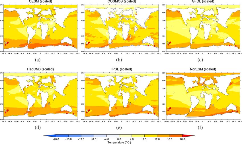
D. J. Lunt et al.: DeepMIP model–data comparison                                                                                 205

pilations (Beerling and Royer, 2011). As such, the Inter-           ematics Coupled Model) is a Coupled Model Intercompari-
governmental Panel on Climate Change (IPCC) concluded               son Project (CMIP) Phase 6 class model and can therefore
that “While recent simulations of the EECO... exhibit a wide        be considered state of the art. In this paper, we present an
inter-model variability, there is generally good agreement be-      ensemble of early Eocene simulations from a range of cli-
tween new simulations and data, particularly if seasonal bi-        mate models, carried out in this framework, and compare
ases in some of the marine SST proxies from high-latitude           them with the latest paleo-data of the EECO. We address the
sites are considered” (Masson-Delmotte et al., 2013). How-          three following key scientific questions in this paper:
ever, more recent work has indicated that early Eocene CO2
concentrations ranged from 1170 ppmv to 2490 ppmv (95 %                 – What are the large-scale features of the DeepMIP
confidence interval) (Anagnostou et al., 2020), which is sub-             Eocene simulations?
stantially lower than the × 16 (4480 ppmv) CCSM3 simula-                – What are the causes of the model spread in these simu-
tion that was the best fit to proxy data of the models examined           lations?
in Lunt et al. (2012).
   Following on from that initial modelling work, two stud-             – How well do the models fit the proxy data, and has there
ies (Sagoo et al., 2013; Kiehl and Shields, 2013) have shown              been an improvement in model fit compared with previ-
that the representation of clouds in models could be modified             ous work?
to give greater polar amplification and climate sensitivity, re-
sulting in simulations that are more consistent with tempera-       2     DeepMIP model simulations
ture proxies of the Eocene at lower CO2 . Kiehl and Shields
(2013) decreased the cloud drop density and increased the           Here, we briefly describe the standard experimental design,
cloud drop radius to represent the effect of reduced cloud          and give a brief description of the model and any departures
condensation nuclei in the Eocene compared with the modern          from the standard experimental design for each model.
simulation, and they obtained good agreement with data at a
CO2 concentration of 1375 ppmv and a CH4 concentration of           2.1    Experimental design
760 ppbv (their “pre-PETM” simulation). Sagoo et al. (2013)
perturbed 10 atmospheric and oceanic variables in an ensem-         The standard experimental design for the DeepMIP model
ble (from which those associated with clouds were judged to         simulations, as well as the underlying motivation, is de-
be the most important) and found that two ensemble mem-             scribed in detail in Lunt et al. (2017). In brief, the simulations
bers were able to simulate temperatures that were in good           consist of a preindustrial control and a number of Eocene
agreement with proxies at a CO2 concentration of 560 ppmv.          simulations at various atmospheric CO2 concentrations (× 3,
Although both of these studies indicated that clouds could          × 6, and × 12 the preindustrial concentration of CO2 , hence-
be the key to reconciling proxies and models, neither of the        forth expressed as × 3, × 6, and × 12 etc, although, in prac-
changes applied were physically based. Furthermore, more            tice, many groups chose different concentrations; see Ta-
recent work has indicated that the response to modifying            ble 1). The paleogeography, vegetation, and river routing for
cloud albedo is very similar to that of increasing CO2 , at least   the Eocene simulations are prescribed according to the re-
in terms of the meridional temperature gradient (Carlson and        constructions of Herold et al. (2014) (see Figs. 3a, b and 4
Caballero, 2017), such that prescribing cloud changes can re-       in Lunt et al., 2017). The solar constant, orbital configura-
sult in a system that is somewhat unconstrained. As such, the       tion, and non-CO2 greenhouse gas concentrations are set to
relevance of these studies for future prediction or to other        preindustrial values. Soil properties are set to homogeneous
paleo-time-periods remains unclear.                                 global mean values derived from the preindustrial simulation,
   To facilitate an intermodel comparison, a standard set           and there are no continental ice sheets in the Eocene simu-
of boundary conditions and a standard experimental design           lations. A suggested initial condition for ocean temperature
have been proposed for a coordinated set of model simula-           and salinity was given, but many groups diverged from this.
tions of the early Eocene (Lunt et al., 2017). In addition, there   The prescription of the calculation of atmospheric aerosols
has been a community effort to better characterize the uncer-       was left to each individual group’s discretion.
tainties in proxy temperature and CO2 estimates of the latest
Paleocene, Paleocene–Eocene thermal maximum (PETM),                 2.2    Individual model simulations
and early Eocene climate optimum (EECO) (Hollis et al.,
2019). Furthermore, some models are available for deep-             An overview of the model simulations is presented in Ta-
time paleoclimate simulations that are more advanced than           bles 1 and S1 in the Supplement. Here, we describe each
those used in the Lunt et al. (2012) study; for example, the        model in turn, and the experimental design of the simulations
Community Earth System Model, version 1.2 (CESM1.2),                if they diverged from that described in Lunt et al. (2017).
includes a more advanced cloud microphysics scheme com-
pared with CCSM3, HadCM3 has a higher ocean resolution
than HadCM3L, and INMCM (Institute of Numerical Math-

https://doi.org/10.5194/cp-17-203-2021                                                             Clim. Past, 17, 203–227, 2021
206                                                                               D. J. Lunt et al.: DeepMIP model–data comparison

Table 1. Summary of the DeepMIP Eocene model simulations described and presented in this paper. In addition to the simulations listed,
each model has an associated preindustrial control. More information about the spin-up of each simulation is given in Table S2. In this paper,
each model is referred to by its short name.

               Model                        Short name     CO2                      CMIP generation      Simulation reference
               CESM1.2_CAM5                 CESM           ×1, ×3, ×6, ×9           CMIP5                Zhu et al. (2019)
               COSMOS-landveg_r2413         COSMOS         × 1, × 3, × 4            CMIP3                This paper
               GFDL_CM2.1                   GFDL           ×1, ×2, ×3, ×4, ×6       CMIP3                This paper
               HadCM3B_M2.1aN               HadCM3         ×1, ×2, ×3               CMIP3                This paper
               INM-CM4-8                    INMCM          ×6                       CMIP6                This paper
               IPSLCM5A2                    IPSL           ×1.5, ×3                 CMIP5                Zhang et al. (2020)
               MIROC4m                      MIROC          ×3                       CMIP3                This paper
               NorESM1_F                    NorESM         ×2, ×4                   CMIP5-6              This paper

2.2.1   CESM (CESM1.2_CAM5)                                              relative humidity threshold for low clouds (rhminl = 0.8975,
                                                                         versus the default value of 0.8875). These code and param-
CESM model description
                                                                         eter changes are not found to alter the present-day climate
The Community Earth System Model version 1.2 (CESM)                      sensitivity in CESM (Zhu et al., 2019).
is used, which consists of the Community Atmosphere
Model 5.3 (CAM), the Community Land Model 4.0 (CLM),                     CESM model simulations
the Parallel Ocean Program 2 (POP), the Los Alamos sea ice
model 4 (CICE), the River Transport Model (RTM), and a                   The CESM Eocene simulations are run at × 1, × 3, × 6,
coupler connecting them (Hurrell et al., 2013). In compar-               and × 9 CO2 concentrations (Table 1). The atmosphere
ison to previous versions of the CESM models that have                   and land have a horizontal resolution of 1.9◦ × 2.5◦ (lati-
been used for Eocene simulation, such as CCSM3 (Hu-                      tude × longitude) with 30 hybrid sigma-pressure levels in the
ber and Caballero, 2011; Winguth et al., 2010; Kiehl and                 atmosphere. The ocean and sea ice are on a nominal 1◦ dis-
Shields, 2013) and CESM1(CAM4) (Cramwinckel et al.,                      placed pole Greenland grid with 60 vertical levels in the
2018), CESM1.2(CAM5) represents a nearly complete over-                  ocean. CAM5 runs with a prognostic aerosol scheme with
haul of the physical parameterizations in the atmosphere                 prescribed preindustrial natural emissions that have been re-
model, including new schemes for radiation, boundary layer,              distributed according to the Eocene paleogeography follow-
shallow convection, cloud microphysics and macrophysics,                 ing the method in Heavens et al. (2012). The vegetation
and aerosols (Hurrell et al., 2013). The new two-moment                  type from Herold et al. (2014) is prescribed in the land
microphysical scheme predicts both the cloud water mix-                  model with active carbon and nitrogen cycling. A modified
ing ratio and particle number concentration. The new aerosol             marginal sea balancing scheme was applied for the Arctic
scheme predicts the aerosol mass and number, and it is cou-              Ocean, which removes any gain or deficit of freshwater over
pled with the cloud microphysics, allowing for the inclu-                the Arctic Ocean and redistributes the mass evenly over the
sion of aerosol indirect effects. The new boundary layer and             global ocean surface excluding the Arctic. This implemen-
shallow convection schemes improve the simulation of shal-               tation conserves ocean salinity and is necessary to prevent
low clouds in the marine boundary layer. These new pa-                   the occurrence of negative salinity that results from high pre-
rameterizations in CAM5 produce a cloud simulation that                  cipitation and river runoff under warm conditions. A similar
agrees much better with satellite observations (Kay et al.,              balancing scheme has been included for marginal seas in all
2012) and a larger present-day equilibrium climate sensi-                of the previously published CESM simulations (Smith et al.,
tivity (∼ 4 ◦ C) than previous versions (∼ 3 ◦ C) (Gettelman             2010). The ocean temperature and salinity were initialized
et al., 2012). CESM1.2(CAM5) reproduces key features of                  from a previous PETM simulation using CCSM3 (Kiehl and
the state and variability of past climates, including the mid-           Shields, 2013). The sea ice model was initialized from a sea-
Piacenzian warm period (Feng et al., 2019), the Last Glacial             ice-free condition. All simulations have been integrated for
Maximum (Zhu et al., 2017a), Heinrich events (Zhu et al.,                2000 model years, with the exception of × 1 which was run
2017b), and the last millennium (Otto-Bliesner et al., 2015;             for 2600 model years.
Thibodeau et al., 2018). To make the model suitable for a
paleoclimate simulation with a high CO2 level, the model
code has been slightly modified to incorporate an upgrade to
the radiation code that corrects the missing diffusivity angle
specifications for certain long-wave bands. As a result of the
code modification, CAM5 has been re-tuned with a different

Clim. Past, 17, 203–227, 2021                                                                  https://doi.org/10.5194/cp-17-203-2021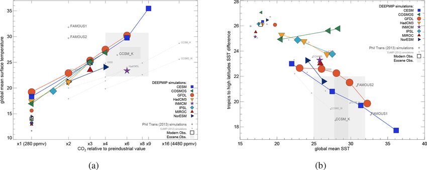
D. J. Lunt et al.: DeepMIP model–data comparison                                                                              207

2.2.2   COSMOS (COSMOS-landveg_r2413)                              2.2.3   GFDL (GFDL_CM2.1)
COSMOS model description                                           GFDL model description
The atmosphere is represented by means of the ECHAM5               These simulations use a modified version of the Geophysi-
(European Centre Hamburg Model) atmosphere general cir-            cal Fluid Dynamics Laboratory (GFDL) CM2.1 model (Del-
culation model (Roeckner et al., 2003). ECHAM5 is based            worth et al., 2006), similar to the late Eocene configuration
on a spectral dynamical core and includes 19 vertical hy-          in Hutchinson et al. (2018, 2019). The ocean component uses
brid sigma-pressure levels. The series of spectral harmon-         the modular ocean model (MOM) version 5.1.0, while the
ics is curtailed via triangular truncation at wave number 31       other components of the model are the same as in CM2.1:
(approx. 3.75◦ × 3.75◦ ). Ocean circulation and sea ice dy-        Atmosphere Model 2, Land Model 2 and the Sea Ice Simu-
namics are computed by the Max-Planck-Institute for Mete-          lator 1. The ocean and sea ice components use a horizontal
orology Ocean Model (MPIOM) ocean general circulation              resolution of 1◦ × 1.5◦ (latitude × longitude). A tripolar grid
model (Marsland et al., 2003) that is employed at 40 un-           is used as in Hutchinson et al. (2018), with a regular latitude–
equally spaced levels on a bipolar curvilinear model grid with     longitude grid south of 65◦ N, a transition to a bipolar Arctic
formal resolution of 3.0◦ × 1.8◦ (longitude × latitude). The       grid north of 65◦ N, and with poles over North America and
coupled ECHAM5–MPIOM model is described by Jung-                   Eurasia. There is no refinement of the latitudinal grid spacing
claus et al. (2006). A concise description of the applica-         in the tropics. The ocean uses 50 vertical levels with the same
tion of the Community Earth System Models (COSMOS)                 vertical spacing as CM2.1. The atmospheric horizontal grid
for paleoclimate studies is given by Stepanek and Lohmann          resolution is 3◦ × 3.75◦ , with 24 vertical levels, as in CM2Mc
(2012). The COSMOS version used here has proven to be a            (Galbraith et al., 2010). This configuration enables relatively
suitable tool for the study of the Earth’s past climate, from      high-resolution ocean and coastlines, with the advantage of
the Holocene (Wei and Lohmann, 2012; Wei et al., 2012;             a faster-running atmosphere. The topography (both land and
Lohmann et al., 2013) and previous interglacials (Pfeiffer and     ocean) uses the 55 Ma reconstruction of Herold et al. (2014),
Lohmann, 2016; Gierz et al., 2017) to glacial (Gong et al.,        re-gridded to the ocean and atmosphere components. Man-
2013; Zhang et al., 2013, 2014; Abelmann et al., 2015; Zhang       ual adjustments are made to ensure that no isolated lakes or
et al., 2017) and tectonic timescales (Knorr et al., 2011;         seas exist and that any narrow ocean straits are at least two
Knorr and Lohmann, 2014; Walliser et al., 2016; Huang              grid cells wide to ensure non-zero velocity fields. The min-
et al., 2017; Niezgodzki et al., 2017; Stärz et al., 2017; Wal-    imum depth of ocean grid cells is 25 m; any shallow ocean
liser et al., 2017; Vahlenkamp et al., 2018; Niezgodzki et al.,    grid cells are deepened to this minimum depth. In the at-
2019). The standard model code of the COSMOS version               mosphere, the topography is smoothed using a three-point
COSMOS-landveg r2413 (2009) is available upon request              mean filter to ensure a smoother interaction with the wind
from the Max Planck Institute for Meteorology in Hamburg           field. This was introduced to remove numerical noise over
(https://www.mpimet.mpg.de, last access: 10 January 2021).         the Antarctic continent, due to the convergence of meridians
                                                                   on the topography grid. Vegetation types are based on Herold
COSMOS model simulations                                           et al. (2014), adapted to the corresponding vegetation type in
                                                                   CM2.1. Aerosol forcing is also adapted from Herold et al.
The COSMOS simulations are carried out at × 1, × 3, and            (2014) to the model, and it is a fixed boundary condition.
× 4 preindustrial CO2 concentrations of 280 ppm. The ocean         Ocean vertical mixing is identical to that in Hutchinson et al.
temperatures in the 3 × CO2 concentration simulation were          (2018) – i.e. a uniform bottom-roughness-enhanced mixing
initialized with uniformly horizontal and vertical tempera-        with a background diffusivity of 1.0 ×10⁻⁵ m2 s−1 .
tures of 10 ◦ C. The initial ocean salinity was set to 34.7 psu.
The simulations with 1 × and 4× CO2 concentrations were
                                                                   GFDL model simulations
restarted from 3 × CO2 after 1000 years. All simulations
were run with transient orbital configurations until the model     The model was initiated from idealized conditions, similar
year 8000. Subsequently, they were run for 1500 years (to          to those outlined in Lunt et al. (2017) with reduced initial
the model year 9500), with fixed, preindustrial orbital pa-        temperatures: T (◦ C) = (5000 − z)/5000 × 25 cos(φ) + 10 if
rameters. All simulations employ the hydrological discharge        z ≤ 5000 m, and T (◦ C) = 10 if z > 5000 m; here, φ is lati-
model of Hagemann and Dümenil (1998) instead of the river          tude, and z is the depth of the ocean (positive downwards).
routing provided by Herold et al. (2014).                          The initial salinity was a constant of 34.7 psu. The above-
                                                                   mentioned initial conditions were used for the × 1, × 2, × 3,
                                                                   and × 4 CO2 experiments. These simulations were initially
                                                                   run for 1500 years, after which the ocean temperatures were
                                                                   adjusted in order to accelerate the approach to equilibrium.
                                                                   This adjustment consisted of calculating the average temper-
                                                                   ature trend for the last 100 years at each model level below

https://doi.org/10.5194/cp-17-203-2021                                                           Clim. Past, 17, 203–227, 2021
208 D. J. Lunt et al.: DeepMIP model–data comparison
500 m, taking a level-by-level global average of this trend, ional temperature gradient and zonal winds and are related
and applying a 1000-year extrapolation uniformly across the to the missing latitudinal variations in the 1D field. Although
ocean at that level. This choice was based on the observation HadCM3 has been used previously to simulate the Pliocene
that all model levels below the mixed layer were consistently (e.g. Lunt et al., 2008, 2010a), the presented simulations
cooling at a slow rate, and the rate of temperature adjust- represent the first published application of HadCM3 to pre-
ment was consistent over a long timescale. After a further Pliocene boundary conditions. However, the lower-resolution
500 years, a second adjustment using the same method was HadCM3L model has been previously used to simulate a
performed. After the second adjustment, all simulations were range of pre-Quaternary climates (e.g. Lunt et al., 2016;
continuously integrated with no further adjustments for a fur- Farnsworth et al., 2019a, b).
ther 4000 years. Thus, the simulations were run for a total
of 6000 years. For the × 6 CO2 experiment, the initial condi- HadCM3 model simulations
tions described above led to transient instabilities due to over-
heating the surface. Thus, the × 6 experiment was instead The HadCM3 simulations are carried out at × 1, ×2, and × 3
initialized using a globally uniform temperature of 19.32 ◦ C. CO2 concentrations. Several ocean gateways were artificially
This represents the same global average temperature as in the widened to allow unrestricted throughflow, and maximum
other experiments and, hence, the same total ocean heat con- water depths in parts of the Arctic Ocean were reduced. The
tent. For the × 6 CO2 , no stepwise adjustments were made; ocean temperatures were initialized from the final state of
the model was run continuously for 6000 years. Eocene model simulations using HadCM3L. The HadCM3L
simulations were set up identically to the corresponding
HadCM3 simulations, but with a lower ocean resolution
2.2.4 HadCM3 (HadCM3B_M2.1aN) (3.75◦ × 2.5◦ as opposed to 1.25◦ × 1.25◦ ). The HadCM3L
simulations were initialized from a similar idealized temper-
HadCM3 model description ature and salinity state as described in Lunt et al. (2017) but
The Hadley Centre Climate Model (HadCM3) simulations with a function that scales with cos2 (lat) rather than cos(lat)
are carried out with the HadCM3B-M2.1aN version of the and overall reduced initial temperatures to ensure numerical
model, as described in detail in Valdes et al. (2017). Equa- stability in tropical regions. Ocean temperatures below 600 m
tions are solved on a Cartesian grid with horizontal resolu- were set to constant values of 4, 8, and 10 ◦ C (at × 1, ×2, and
tions of 3.75◦ × 2.5◦ in the atmosphere and 1.25◦ × 1.25◦ × 3 CO2 respectively) based on results from previous Ypre-
in the ocean with 19 and 20 vertical levels respectively. A sian simulations. The HadCM3 simulations were branched
few changes are made to the version described in Valdes off from the respective HadCM3L integrations after 4400 to
et al. (2017) to make it suitable for deep-time paleoclimate 4900 years of spin up and run for a further 2950 years. The
modelling: (a) a salinity flux correction is applied to the initial 50 years of all HadCM3 runs used the simplified verti-
global ocean (at all model depths) in order to conserve salin- cal diffusion scheme from HadCM3L (Valdes et al., 2017) to
ity; (b) the various modern-specific parameterizations in the reduce numerical problems caused by the changed horizon-
ocean model are turned off, such as those associated with tal ocean resolution. The remaining years of the runs use the
the Mediterranean and Hudson Bay outflow and the North standard HadCM3 diffusion scheme (Valdes et al., 2017).
Atlantic mixing; and (c) a prognostic 1D ozone scheme is
used instead of a fixed vertical profile of ozone. The standard 2.2.5 INMCM (INM-CM4-8)
configuration uses a prescribed ozone climatology which is a
INMCM model description
function of latitude, height, and month of the year that does
not change with climate and can become numerically unsta- The INMCM simulations are carried out with the INM-
ble at high CO2 levels. The prognostic ozone scheme uses CM48 (INM-CM4-8) version of the model, as described in
the diagnosed model tropopause height to assign three dis- Volodin et al. (2018). The INM-CM4-8 climate model has
tinct ozone concentrations for the troposphere, tropopause, a horizontal resolution of 2◦ × 1.5◦ in the atmosphere; a to-
and stratosphere (2.0 ×10⁻⁸ , 2.0 ×10⁻⁷ , and 5.5 ×10⁻⁶ , in tal of 17 vertical sigma levels up to a value of 0.01 (about
mass mixing ratio, respectively). This allows for a dynamic 30 km) are used for the Eocene experiment, and 21 levels are
update of the 1D ozone field in response to the thermally used for the preindustrial experiment. The equations of the
driven vertical expansion of the troposphere. Absolute val- atmosphere dynamics are solved by finite difference meth-
ues for the three levels are chosen to minimize the effects ods. The parameterizations of physical processes correspond
on the global mean and overall tropospheric temperature to the INM-CM5 model (Volodin et al., 2017). Parameteri-
changes compared with the standard 2D climatology. Con- zation of condensation and cloud formation follows Tiedtke
centrations at the uppermost model level are fixed to the (1993). Cloud water is a prognostic variable. Parameteriza-
higher stratospheric value to constrain the lower bound of tion of the cloud fraction follows Smagorinsky (1963); cloud
total stratospheric ozone. Significant differences to the stan- fraction is a diagnostic variable. The surface, soil, and veg-
dard configuration are limited to the stratospheric merid- etation scheme follows Volodin and Lykossov (1998). The
Clim. Past, 17, 203–227, 2021 https://doi.org/10.5194/cp-17-203-2021D. J. Lunt et al.: DeepMIP model–data comparison 209
evolution of the equations for temperature, soil water, and CM5A2 on preindustrial and historical climates are fully de-
soil ice are solved at 23 levels from the surface to 10 m scribed in Sepulchre et al. (2020). Sepulchre et al. (2020)
depth. The fractional area of 13 types of potential vegetation also provide a description of the technical changes that were
is specified. Actual vegetation and the leaf area index (LAI) implemented in IPSL-CM5A2 to carry out deep-time pale-
are calculated according to the soil water content in the root oclimate simulations. In particular, the tripolar mesh grid on
zone and soil temperature. This model also contains a car- which NEMO runs has been modified to ensure that there are
bon cycle and an aerosol scheme (Volodin and Kostrykin, no singularity points within the ocean domain. Modern pa-
2016), taking the direct impact of aerosols on radiation into rameterizations of water outflows across specific straits, such
account, as well as the first indirect effect (the influence of as the Gibraltar or Red Sea straits, are also turned off.
aerosols on the condensation rate). The concentration of 10
types of aerosol and their radiative properties are calculated IPSL model simulations
interactively. In the ocean component, the resolution of the
INM-CM4-8 model is 1.0◦ × 0.5◦ (longitude × latitude) and The IPSL simulations are run at × 1.5 and × 3 CO2 concen-
has 40 sigma levels vertically. Finite difference equations are trations. The bathymetry is obtained from the Herold et al.
solved on a generalized spherical C-grid with the North Pole (2014) dataset, with additional manual corrections in some
shifted to Siberia; the South Pole is in the same place as the locations, for instance in the West African region, to main-
geographical pole. tain sufficiently large oceanic straits. Modern boundary con-
ditions of NEMO include forcings of the dissipation asso-
INMCM model simulations ciated with internal wave energy for the M2 and K1 tidal
components (de Lavergne et al., 2019). The parameteriza-
The INM-CM4-8 Eocene simulation is carried out at a × 6 tion follows Simmons et al. (2004) with refinements in the
CO2 concentration. The INM-CM4-8 simulation was ini- modern Indonesian throughflow (ITF) region according to
tialized from a similar idealized temperature and salinity Koch-Larrouy et al. (2007). To create an early Eocene tidal
state as described in Lunt et al. (2017), but the initial for- dissipation forcing, the Herold et al. (2014) M2 tidal field
mula for the ocean temperature is modified as follows: T = (obtained from the tidal model simulations of Green and
((5000−z)/5000×20 cos(φ))+15, thereby reducing the ini- Huber, 2013) is directly interpolated onto the NEMO grid
tial temperatures to ensure numerical stability in tropical using bilinear interpolation. In the absence of any estima-
regions. The 27 biomes were converted into the 13 model tion for the early Eocene, the K1 tidal field is prescribed
types of vegetation. The duration for the Eocene simulation as zero. In addition, the parameterization of Koch-Larrouy
is 1150 years. Output data are averaged over the years from et al. (2007) is not used here because the ITF does not ex-
1051 to 1150. ist in the early Eocene. The geothermal heating distribution
is created from the 55 Ma global crustal age distribution of
2.2.6 IPSL (IPSLCM5A2) Müller et al. (2008), on which the age–heat flow relation-
ship of the Stein and Stein (1992) model is applied: q(t) =
IPSL model description
510×t −1/2 if t ≤ 55 Ma, and q(t) = 48+96 exp(−0.0278×t)
The Institut Pierre Simon Laplace (IPSL) simulations are if t > 55 Ma. In regions of subducted seafloor where age in-
performed with the IPSL-CM5A2 Earth system model formation is not available, the minimal heat flow value is
(Sepulchre et al., 2020). IPSL-CM5A2 is based on the prescribed, which is derived from a known crustal age. The
CMIP5-generation previous IPSL Earth system model IPSL- resulting 1◦ × 1◦ field is then bilinearly interpolated onto
CM5A (Dufresne et al., 2013) but includes new revisions the NEMO grid. It must be noted that the Stein and Stein
of each components, a re-tuning of global temperature, and (1992) parameterization becomes singular for young crustal
technical improvements to increase computing efficiency. It ages and yields unrealistically large heat flow values. Fol-
consists of the LMDZ5 (Laboratoire de Meétéorologie Dy- lowing Emile-Geay and Madec (2009), an upper limit of
namique Zoom) atmosphere model, the Organising Carbon 400 mW m−2 is set for heat flow values after the interpola-
and Hydrology In Dynamic Ecosystems (ORCHIDEE) land tion procedure. Salinity is initialized as globally constant to
surface and vegetation model and the Nucleus for European a value of 34.7 psu following Lunt et al. (2017). The initial-
Modeling of the Ocean (NEMOv3.6) ocean model, which ization of the model with the proposed DeepMIP tempera-
includes the LIM2 sea ice model and the Pelagic Interac- ture distribution (Lunt et al., 2017) led to severe instabili-
tions Scheme for Carbon and Ecosystem Studies (PISCES- ties in the model during the spin-up phase. Thus, the ini-
v2) biogeochemical model. LMDZ5 and ORCHIDEE run at tial temperature distribution has been modified as follows:
a horizontal resolution of 1.9◦ × 2.5◦ (latitude × longitude) T (◦ C) = (1000−z)/1000×25 cos(φ)+10 if z ≤ 1000 m, and
with 39 hybrid sigma-pressure levels in the atmosphere. T (◦ C) = 10 if z > 1000 m; here, φ is the latitude, and z is the
NEMO runs on a tripolar grid at a nominal resolution of depth of the ocean (metres below surface). This new equation
2◦ , enhanced up to 0.5◦ at the Equator, with 31 vertical lev- gives an initial globally constant temperature of 10 ◦ C below
els in the ocean. The performances and evaluation of IPSL- 1000 m and a zonally symmetric distribution above 1000 m,
https://doi.org/10.5194/cp-17-203-2021 Clim. Past, 17, 203–227, 2021210 D. J. Lunt et al.: DeepMIP model–data comparison
reaching surface values of 35 ◦ C at the Equator and 10 ◦ C ear damping. This damping and all isolated basins and lakes
at the poles. This corresponds to a 5 ◦ C surface temperature are removed in the DeepMIP simulation.
reduction compared with DeepMIP guidelines (Lunt et al.,
2017). No sea ice is prescribed at the beginning of the sim- MIROC model simulations
ulations. In IPSL-CM5A2, the NEMO ocean model is inher-
ently composed of the PISCES biogeochemical model. Bio- Out of the three standard DeepMIP simulations, MIROC is
geochemical cycles and marine biology are directly forced used with a × 3 CO2 concentration only and run for 5000
by dynamical variables of the physical ocean and may affect model years. The atmosphere is initialized from a previous
the ocean physics via its influence on chlorophyll produc- experiment without ice sheets and with a × 2 CO2 concen-
tion, which modulates light penetration in the ocean. How- tration. For the initial ocean state, salinity is set to a con-
ever, because this feedback does not much affect the ocean stant value of 34.7 psu, as recommended in Lunt et al. (2017).
state (Kageyama et al., 2013) and because the early Eocene However, the ocean temperatures are 15 ◦ C cooler than those
mean ocean colour is unknown, a constant chlorophyll value recommended – i.e. T (◦ C) = (5000 − z)/5000 × 25 cos(φ) if
of 0.05 g Chl L−1 is prescribed for the computation of light z ≤ 5000 m, and T (◦ C) = 0 if z > 5000 m. Previous MIROC
penetration in the ocean. As a consequence, marine biogeo- experiments similar to this × 3 CO2 DeepMIP simulation
chemical cycles and biology do not alter the dynamics of the show that this initialization should be much closer to the fi-
ocean; as such, the biogeochemical initial and boundary con- nal climate state. Simulations were also carried out at × 1
ditions have been kept at modern values. The topographic and × 2, but they are not discussed in this paper.
field is created from the Herold et al. (2014) topographic
dataset; LMDZ includes a sub-grid-scale orographic drag pa- 2.2.8 NorESM (NorESM1_F)
rameterization that requires high-resolution surface orogra-
NorESM model description
phy (Lott and Miller, 1997; Lott, 1999). A similar procedure
is applied for the standard deviation of orography provided The Norwegian Earth System Model (NorESM) simula-
by Herold et al. (2014). Aerosol distributions are left identi- tions are carried out with the NorESM1-F version of the
cal to preindustrial values. The × 3 simulation is initialized model, which is described in detail in Guo et al. (2019). The
from rest and run for 4000 years. The × 1.5 simulation is NorESM version that contributes to CMIP5 is NorESM1-
branched from the model year 1500 of the × 3 simulation M. It has a ∼ 2◦ resolution atmosphere and land configu-
and run for 4000 years. The × 1.5 and × 3 simulations are ration and a nominal 1◦ ocean and sea ice configuration.
identical to those presented in Zhang et al. (2020). In NorESM1-F, the same atmosphere–land grid is used as
in NorESM1-M (CMIP5 version), whereas a tripolar grid is
used for the ocean–sea ice components in NorESM1-F, in-
2.2.7 MIROC (MIROC4m)
stead of the bipolar grid in NorESM1-M. The tripolar grid
MIROC model description is also used in the CMIP6 version of NorESM (NorESM2).
NorESM1-F runs about 2.5 times faster than NorESM1-
The version of the Model for Interdisciplinary Research on M. For the preindustrial simulation, NorESM-F has a more
Climate (MIROC) used here is MIROC4m, a mid-resolution realistic Atlantic Meridional Overturning Circulation than
model composed of atmosphere, land, river, sea ice, and NorESM1-M.
ocean components. Full documentation of the model can be
found in K-1 model developers (2004) and is summarized NorESM model simulations
in Chan et al. (2011). The atmosphere has a horizontal res-
olution of T42 and 20 vertical sigma levels. Details of the The NorESM simulations are carried out at × 2 and × 4 CO2
land surface model, Minimal Advanced Treatments of Sur- concentrations. The ocean temperatures were initialized from
face Interaction and Runoff (MATSIRO), can be found in the × 2 CO2 Eocene simulations with the lower-resolution
Takata et al. (2003). The ocean component is basically ver- NorESM-L model (Zhang et al., 2012). The ocean salinity
sion 3.4 of the CCSR (Center for Climate System Research) was initialized with constant values of 25.5 psu in the Arc-
Ocean Component Model (COCO); the reader is referred to tic and 34.5 psu elsewhere. From the initial conditions, the
Hasumi (2000) for details. The horizontal resolution is set to × 2 CO2 experiment was run for 2100 years in total. The
256 × 196 (longitude × latitude), with a higher resolution in × 4 CO2 was branched from the end of the 100th year of the
the tropics, and the vertical resolution is set to 44 levels, with × 2 CO2 experiment and was run for 2000 years. The results
the top 8 levels in sigma coordinates. Present-day bathymetry from the last 100 years were used in the study. Note that the
is derived from Earth topography five minute grid (ETOPO5) NorESM simulations were carried out with the Baatsen et al.
data. For present-day experiments, areas of water such as (2016) paleogeography (based on a paleomagnetic reference
Hudson Bay and the Mediterranean Sea are represented as frame), not the Herold et al. (2014) paleogeography (based
isolated basins. As such, ocean salinity and heat are artifi- on a mantle reference frame), in contrast to the other simula-
cially exchanged with the open ocean through a two-way lin- tions described in this paper.
Clim. Past, 17, 203–227, 2021 https://doi.org/10.5194/cp-17-203-2021D. J. Lunt et al.: DeepMIP model–data comparison 211
3 Results It is also worth noting that some models crashed when run
under CO2 concentrations higher than in the simulations de-
We discuss the results from the model simulations, focusing scribed here. In particular, CESM crashed at × 12, COSMOS
on the model spin-up and equilibrium (Sect. 3.1) followed crashed at × 6, HadCM3 crashed at × 4, IPSL crashed at × 6,
by three aspects which align with the research questions out- and MIROC crashed at × 4. These crashes have not been ex-
lined at the end of Sect. 1: the large-scale features of the plored in detail, but they could be due to feedbacks becoming
modelled temperature response compared with those of the more positive as temperature increases (for example associ-
preindustrial period (Sect. 3.2), the reasons for the different ated with an increase in height of the tropopause; Meraner
model responses (Sect. 3.3), and a comparison with paleo- et al., 2013); this could occur to such an extent that positive
proxy data (Sect. 3.4). feedbacks overcome the negative Planck feedback (Bloch-
Johnson et al., 2015), at which point a “runaway” phase is
3.1 Model spin-up and equilibrium entered and the temperature begins to increase rapidly. This
can then cause a violation of the Courant–Friedrichs–Lewy
It is important to assess the extent to which the Eocene sim- (CFL) criterion due to high wind speeds associated with the
ulations represent an equilibrated state. This is because the generation of large pressure and/or temperature gradients,
initial condition may be far from the ultimate equilibrium for causing the model to crash.
many models; as such, very long simulations are required to
reach this equilibrium, which may be prohibitive in terms
of computation and time resources. For all of the Deep- 3.2 Documentation of large-scale features
MIP simulations, the length as well as the top-of-atmosphere Here, we present the large-scale features of the DeepMIP
(TOA) imbalance and near-surface global mean air temper- simulations, with a focus on annual mean temperature. We
ature trend at the end of the simulation are summarized in start with global mean quantities, move on to latitudinal gra-
Table S1. The TOA imbalance and temperature trends are dients, and finish by describing the spatial patterns.
also given for the associated preindustrial simulations. As Figure 1a shows the global mean near-surface air temper-
part of the DeepMIP experimental design (Lunt et al., 2017) ature as a function of model CO2 for each DeepMIP simu-
– and formulated before any simulations had started run- lation and associated preindustrial control as well as some
ning – it was suggested that appropriate criteria for suffi- previous Eocene simulations carried out with other boundary
cient model equilibration would be that simulations should conditions (Lunt et al., 2012; Kiehl and Shields, 2013; Sa-
ideally be “(a) at least 1000 years in length, and (b) have goo et al., 2013). The DeepMIP simulations are fairly con-
an imbalance in the top-of-atmosphere net radiation of less sistent in terms of global mean temperature for a given CO2
than 0.3 W m−2 (or have a similar imbalance to that of the concentration across the ensemble. The exception to this is
preindustrial control), and (c) have sea surface temperatures INMCM, which at × 6 CO2 has a lower global mean temper-
that are not strongly trending (less than 0.1 ◦ C per century in ature than any of the × 3 simulations. This is consistent with
the global mean).”. All the simulations satisfy criterion (a). the fact that INMCM has the lowest climate sensitivity of all
All simulations except for CESM (× 3, × 6, and × 9) and the models in the CMIP6 ensemble (Zelinka et al., 2020).
IPSL (× 1.5 and × 3) satisfy criterion (b). Note that for some With the exception of INMCM, the spread in the DeepMIP
models, the preindustrial TOA imbalance is relatively large; simulations is substantially less than in the previous Eocene
this may be due to non-conservation of energy (e.g. COS- simulations. In particular, at × 3 CO2 , the CESM, COSMOS,
MOS; Stevens et al., 2013) or owing to the fact that some GFDL, HadCM3, IPSL, and MIROC simulations are within
energy fluxes are calculated at the top of the model rather 1.9 ◦ C, compared with 5.0 ◦ C at × 4 for the previous simu-
than at the top of the atmosphere (e.g. INMCM); in these lations. Part of the reason for the reduced spread of many
cases, the TOA imbalance is not a good diagnostic for equi- of the DeepMIP simulations compared with previous simula-
libration because there is some atmosphere above the top of tions may be related to the fact that all of the DeepMIP model
the model that can interact with incoming or outgoing radi- simulations have the same prescribed paleogeography, land–
ation (i.e. the model top is not at 0 mbar). All of the models sea mask, and vegetation, whereas previous simulations used
except for CESM (× 3), COSMOS (× 4), and HadCM3 (× 2 a variety of these boundary conditions.
and × 3) satisfy criterion (c). Overall, all of the models sat- The DeepMIP models have a range of Eocene climate sen-
isfy at least two of the three criteria, except for CESM at × 3 sitivities to CO2 doubling: from a minimum of 2.9 ◦ C (for
which is nonetheless close to both missed criteria (0.32 ver- NorESM) to a maximum of 5.6 ◦ C (for IPSL, excluding the
sus 0.30 W m−2 and 1.1 versus 1.0 ◦ C). As such, we make a anomalously warm × 9 CESM simulation). The average of
decision to accept all simulations as being sufficiently equi- the DeepMIP climate sensitivities (again excluding the × 9
librated and to include them in the ensemble; however, note CESM simulation) is 4.5 ◦ C, which is greater than the av-
that further spin-up would be required to confirm the results erage of the previous simulations (3.3 ◦ C). There is a non-
of those simulations with relatively large residual trends or linearity (i.e. a global mean temperature that increases with
anomalous TOA imbalances. CO2 differently than would be expected from a purely log-
https://doi.org/10.5194/cp-17-203-2021 Clim. Past, 17, 203–227, 2021212 D. J. Lunt et al.: DeepMIP model–data comparison Figure 1. (a) Global annual mean near-surface (2 m) air temperature in the DeepMIP simulations, as a function of atmospheric CO2 . Large coloured symbols show the Eocene simulations, and smaller coloured symbols show the associated preindustrial controls. Also shown are results from some previous Eocene simulations (Lunt et al., 2012; Kiehl and Shields, 2013; Sagoo et al., 2013) and associated preindustrial control simulations (small grey symbols). The models that have carried out Eocene simulations at more than one CO2 concentration are joined by a straight line. The open square shows modern observations. The grey filled boxes show estimates of the global mean temperature (from Inglis et al., 2020) and CO2 (from Anagnostou et al., 2020) derived from proxies. For temperature, the light grey box shows the 10 % to 90 % confidence interval and the dark grey box shows the 33 % to 66 % confidence interval; for CO2 , the light grey box shows ±1 SD and the dark grey box shows ±2 SD; see Sect. 3.4 for more details. Panel (b) is the same as panel (a) but for the meridional SST gradient as a function of global mean SST. The meridional SST gradient is defined here as the average SST equatorwards of ±30◦ minus the average SST polewards of ±60◦ . The grey filled boxes show estimates of the global mean SST (from Inglis et al., 2020) and SST gradient (from Cramwinckel et al., 2018; Evans et al., 2018; Zhu et al., 2019) derived from proxies. For SST, the light grey box shows the 10 % to 90 % confidence interval and the dark grey box shows the 33 % to 66 % confidence interval; for the meridional temperature gradient, the light grey box shows the range (which extends below the y axis limit, down to 14 ◦ C); see Sect. 3.4 for more details. arithmic relationship) in the CESM model simulations (as The latitudinal gradient of SST, defined here as the average previously noted by Zhu et al., 2019) as well as in HadCM3 SST equatorwards of ±30◦ minus the average temperature and (to a lesser extent) GFDL and COSMOS. In CESM, the polewards of ±60◦ , is shown in Fig. 1b. All DeepMIP models climate sensitivity, normalized to a CO2 doubling, increases that have carried out simulations at more than one CO2 con- from 4.2 ◦ C at × 1 to 4.8 and 9.7 ◦ C at × 3 and × 6 respec- centration show a decrease in the meridional SST gradient tively. In GFDL, the climate sensitivity increases from 3.7 ◦ C as temperature increases, apart from COSMOS. COSMOS at × 1 to 5.1 ◦ C at × 3, but it then decreases to 4.7 ◦ C at × 4. also has the strongest preindustrial meridional temperature In HadCM3, the climate sensitivity increases from 3.8 ◦ C at gradient. The × 1 CO2 Eocene simulations indicate that the × 1 to 6.6 ◦ C at × 2. In COSMOS, the climate sensitivity de- non-CO2 DeepMIP boundary conditions decrease the latitu- creases from 5.2 ◦ C at × 1 to 4.2 ◦ C at × 3. In CESM, the dinal gradient by 3.4 ◦ C for GFDL, 3.3 ◦ C for CESM, 2.1◦ non-linearity has been shown to arise from an increase in the for COSMOS, and 0.8 ◦ C for HadCM3. The GFDL model strength of the positive short-wave cloud feedback as a func- displays a markedly non-linear response, with a more rapidly tion of temperature (Zhu et al., 2019); this is most apparent decreasing temperature gradient as a function of temperature in the transition from × 6 to × 9. at higher temperatures than at lower temperatures. In con- CESM, COSMOS, GFDL, and HadCM3 all carried out trast to the global mean temperature, the DeepMIP models simulations at × 1 CO2 ; comparison with the associated show substantial spread in the meridional temperature gradi- preindustrial controls indicates that the non-CO2 compo- ent across the ensemble; COSMOS has a particularly strong nent of global warmth (i.e. due to changes in paleogeogra- gradient in the Eocene at × 3 and × 4 CO2 , and HadCM3 and phy, vegetation, and aerosols, and the removal of continen- IPSL also have relatively strong gradients, similar to previ- tal ice sheets) is 5.1, 3.6, 3.5, and 3.1 ◦ C for CESM, GFDL, ous Eocene simulations with HadCM3L (Lunt et al., 2010b). HadCM3, and COSMOS respectively. This is for compari- The zonal mean near-surface air temperature anomaly, rel- son with previous simulations using CCSM3 (Caballero and ative to the preindustrial simulation, as a function of latitude Huber, 2013) that indicated a non-CO2 warming of ∼ 5◦ C. is shown in Fig. 2. Polar amplification is clear in both hemi- Clim. Past, 17, 203–227, 2021 https://doi.org/10.5194/cp-17-203-2021
D. J. Lunt et al.: DeepMIP model–data comparison 213
Figure 2. Zonal mean near-surface air temperatures in the DeepMIP simulations, as a function of latitude and prescribed atmospheric CO2
concentration, expressed as anomalies relative to the equivalent preindustrial control for (a) CESM, (b) COSMOS, (c) GFDL, (d) HadCM3,
(e) INMCM, (f) IPSL, (g) MIROC, and (h) NorESM.
spheres for all models at CO2 > × 1. There is greater am- warming over land than over ocean. Many of the continen-
plification in the Southern Hemisphere than in the North- tal regions where the warming is more muted (such as the
ern Hemisphere, due to the replacement of the Antarctic Rockies, tropical east Africa, India, and the mid-latitudes of
ice sheets with vegetated land surface, with associated local East Asia) are associated with regions of high topography in
warming due to the altitude and albedo change. There is a the Eocene. There is also substantial warming in the North
similar pattern of response across the models for a given CO2 Pacific in all simulations. This may be associated with deep-
concentration. However, although the models have a similar water formation in this region driving poleward heat trans-
response in the Southern Hemisphere, the CESM model has port in the Pacific, but the ocean circulation in these simula-
greater polar amplification than other models in the Northern tions will be explored in a subsequent study.
Hemisphere for a given CO2 concentration (in particular at A similar plot, but without the zonal mean of the prein-
× 3 CO2 ). The pattern of warming in the × 1 simulations is dustrial simulation (i.e. GATm m
e −GATp ), is shown in Fig. S1.
similar between the CESM, GFDL, and HadCM3 models. In Figure S1 also includes the Eocene simulations at × 1 and
particular, they all exhibit warming around 30–40◦ N, which × 1.5. The Eocene × 1 simulations minus the preindustrial
coincides with lower topography in the Tibetan Plateau re- simulations show the spatial impact of the changes to the
gion in the Eocene relative to the preindustrial period. There non-CO2 boundary conditions. Consistent across the ensem-
is also consistent warming in the Northern Hemisphere Arc- ble is the clear warming in Antarctica associated with the
tic (except for COSMOS) that coincides with the absence of altitude and albedo change, warming in the Tibetan Plateau
the Greenland ice sheet and boreal forest in place of tundra associated with altitude change, and cooling in Europe.
and bare soil in the preindustrial period. The same underly-
ing structure is seen in the higher CO2 simulations (see, for 3.3 Reasons for model spread
example, GFDL, Fig. 2b).
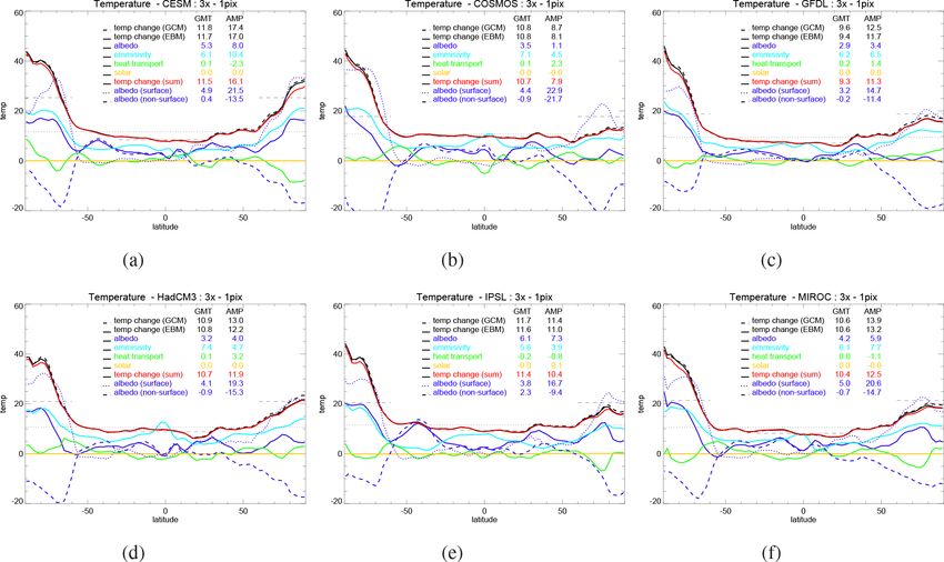
The spatial pattern of surface air temperature response is Here, we first qualitatively explore the different model results
shown in Fig. 3. Because of the variation in continental posi- by presenting the changes in albedo and emissivity across
tions between the preindustrial and Eocene periods, we show the ensemble. We then quantitatively relate these to the zonal
the difference between the Eocene and the zonal mean of mean temperature change and global metrics by making use
the preindustrial simulation, i.e. GATm m of a 1D energy balance framework. Future work in the frame-
e − GATp in the no-
tation of Lunt et al. (2012). This shows some consistent re- work of DeepMIP will explore the model simulations in more
sponses across the ensemble. In particular, in addition to the detail, in particular the response of clouds, the hydrological
polar amplification, the response is characterized by greater cycle, and ocean circulation.
https://doi.org/10.5194/cp-17-203-2021 Clim. Past, 17, 203–227, 2021You can also read