Description of the multi-approach gravity field models from Swarm GPS data - GFZpublic
←
→
Page content transcription
If your browser does not render page correctly, please read the page content below
Earth Syst. Sci. Data, 12, 1385–1417, 2020
https://doi.org/10.5194/essd-12-1385-2020
© Author(s) 2020. This work is distributed under
the Creative Commons Attribution 4.0 License.

         Description of the multi-approach gravity field models
                         from Swarm GPS data
           João Teixeira da Encarnação1,2 , Pieter Visser1 , Daniel Arnold3 , Aleš Bezdek4 , Eelco Doornbos5 ,
               Matthias Ellmer6 , Junyi Guo8 , Jose van den IJssel1 , Elisabetta Iorfida1 , Adrian Jäggi3 ,
            Jaroslav Klokocník4 , Sandro Krauss7 , Xinyuan Mao3 , Torsten Mayer-Gürr7 , Ulrich Meyer3 ,
                 Josef Sebera4 , C. K. Shum8 , Chaoyang Zhang8 , Yu Zhang8 , and Christoph Dahle9,3
                   1 Faculty      of Aerospace Engineering, Delft University of Technology, Kluyverweg 1,
                                                 2629 HS, Delft, the Netherlands
        2 Center for Space Research, The University of Texas at Austin, 3925 West Braker Lane, Suite 200 Austin,

                                                      TX 78759-5321, USA
                   3 Astronomical Institute of the University of Bern, Sidlerstrasse 5, 3012 Bern, Switzerland
        4 Astronomical Institute of the Czech Academy of Sciences, Fricova 298, 251 65 Ondřejov, Czech Republic
            5 Royal Netherlands Meteorological Institute, Utrechtseweg 297, 3731 GA De Bilt, the Netherlands
                         6 Jet Propulsion Laboratory, 4800 Oak Grove Drive, Pasadena, CA 91109, USA
             7 Institute of Geodesy of the Graz University of Technology, Steyergasse 30/III, 8010 Graz, Austria
           8 School of Earth Sciences of The Ohio State University, 125 Oval Dr S, Columbus, OH 43210, USA
                                9 GFZ German Research Centre for Geosciences, Potsdam, Germany

                 Correspondence: João Teixeira da Encarnação (j.g.deteixeiradaencarnacao@tudelft.nl)

                               Received: 2 September 2019 – Discussion started: 1 October 2019
                          Revised: 18 April 2020 – Accepted: 21 April 2020 – Published: 22 June 2020

      Abstract. Although the knowledge of the gravity of the Earth has improved considerably with CHAMP,
      GRACE, and GOCE (see appendices for a list of abbreviations) satellite missions, the geophysical commu-
      nity has identified the need for the continued monitoring of the time-variable component with the purpose of
      estimating the hydrological and glaciological yearly cycles and long-term trends. Currently, the GRACE-FO
      satellites are the sole dedicated provider of these data, while previously the GRACE mission fulfilled that role
      for 15 years. There is a data gap spanning from July 2017 to May 2018 between the end of the GRACE mission
      and start the of GRACE-FO, while the Swarm satellites have collected gravimetric data with their GPS receivers
      since December 2013.
         We present high-quality gravity field models (GFMs) from Swarm data that constitute an alternative and inde-
      pendent source of gravimetric data, which could help alleviate the consequences of the 10-month gap between
      GRACE and GRACE-FO, as well as the short gaps in the existing GRACE and GRACE-FO monthly time series.
         The geodetic community has realized that the combination of different gravity field solutions is superior to
      any individual model and set up the Combination Service of Time-variable Gravity Fields (COST-G) under the
      umbrella of the International Gravity Field Service (IGFS), part of the International Association of Geodesy
      (IAG). We exploit this fact and deliver the highest-quality monthly GFMs, resulting from the combination of
      four different gravity field estimation approaches. All solutions are unconstrained and estimated independently
      from month to month.
         We tested the added value of including kinematic baselines (KBs) in our estimation of GFMs and conclude
      that there is no significant improvement. The non-gravitational accelerations measured by the accelerometer on
      board Swarm C were also included in our processing to determine if this would improve the quality of the GFMs,
      but we observed that is only the case when the amplitude of the non-gravitational accelerations is higher than
      during the current quiet period in solar activity.

Published by Copernicus Publications.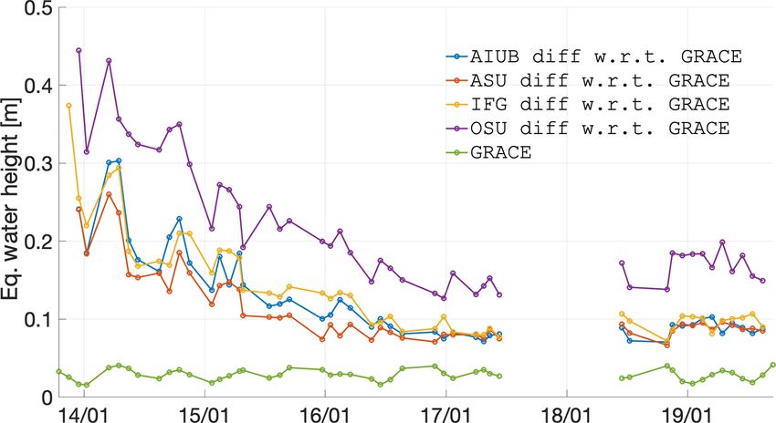
1386                        J. Teixeira da Encarnação et al.: Description of the gravity field models from Swarm GPS data

          Using GRACE data for comparison, we demonstrate that the geophysical signal in the Swarm GFMs is largely
       restricted to spherical harmonic degrees below 12. A 750 km smoothing radius is suitable to retrieve the temporal
       variations in Earth’s gravity field over land areas since mid-2015 with roughly 4 cm equivalent water height
       (EWH) agreement with respect to GRACE. Over ocean areas, we illustrate that a more intense smoothing with
       3000 km radius is necessary to resolve large-scale gravity variations, which agree with GRACE roughly at the
       level of 1 cm EWH, while at these spatial scales the GRACE observes variations with amplitudes between 0.3
       and 1 cm EWH. The agreement with GRACE and GRACE-FO over nine selected large basins under analysis is
       0.91 cm, 0.76 cm yr−1 , and 0.79 in terms of temporal mean, trend, and correlation coefficient, respectively.
          The Swarm monthly models are distributed on a quarterly basis at ESA’s Earth Swarm Data Access (at
       https://swarm-diss.eo.esa.int/, last access: 5 June 2020, follow Level2longterm and then EGF) and at the Inter-
       national Centre for Global Earth Models (http://icgem.gfz-potsdam.de/series/02_COST-G/Swarm, last access:
       5 June 2020), as well as identified with the DOI https://doi.org/10.5880/ICGEM.2019.006 (Encarnacao et al.,
       2019).

1   Introduction                                                  et al., 2004) was by far the most important space-borne
                                                                  global provider of the needed data for the period from
                                                                  April 2002 until July 2017. GRACE Follow-On (GRACE-
Swarm is the fifth Earth Explorer mission by the Euro-
                                                                  FO) was launched in May 2018 and is expected to continue
pean Space Agency (ESA), launched on 22 November 2013
                                                                  the high-quality observation of Earth’s time-variable gravity
(Haagmans, 2004; Friis-Christensen et al., 2008). Its primary
                                                                  field for at least 5 years (Flechtner et al., 2016). Thus a time
objective is to provide the best ever survey of the Earth’s
                                                                  gap exists between the GRACE and GRACE-FO missions,
magnetic field and its temporal variations as well as the elec-
                                                                  and, importantly, no missions have yet been selected for the
tric field of the atmosphere (Olsen et al., 2013). Swarm con-
                                                                  post-GRACE-FO period. It can thus be claimed that the only
sists of three identical satellites, two flying in a pendulum
                                                                  guarantee for sustained observation of time-variable gravity
formation (side by side, converging near the poles) at an ini-
                                                                  from space is constituted by space-borne GPS receivers on
tial altitude of about 470 km and one at an altitude of about
                                                                  LEO satellites. Moreover, the associated data can be used to
520 km, all in near-polar orbit. In addition to a sophisticated
                                                                  fill the gap between the GRACE and GRACE-FO missions
instrument suite for observing the geomagnetic and electric
                                                                  (be it with a different quality in terms of spatial and tem-
fields, the Swarm satellites are equipped with high-precision,
                                                                  poral resolution). The measurement of Earth’s gravitational
dual-frequency Global Positioning System (GPS) receivers,
                                                                  changes with Swarm is further motivated by (i) the need to
star trackers, and accelerometers. Many recent studies and
                                                                  increase the accuracy of global mass estimates in order to
activities have shown the feasibility of observing the Earth’s
                                                                  properly quantify global sea-level rise and (ii) the opportu-
gravity field and its long-wavelength temporal variations
                                                                  nity to provide independent estimates of temporal variations
with high-quality GPS receivers on board low-Earth orbit
                                                                  in low-degree coefficients, in particular related to C2,0 and
(LEO) satellites (Zehentner and Mayer-Gürr, 2014; Bezdek
                                                                  C3,0 , which are weakly observed by GRACE. Under this mo-
et al., 2016; Dahle et al., 2017). For Swarm, Teixeira da En-
                                                                  tivation, this paper aggregates a series of studies and analy-
carnação et al. (2016) successfully demonstrated the obser-
                                                                  ses that, respectively, motivate our processing choices and
vation of long-wavelength temporal gravity. They produced
                                                                  demonstrate the capabilities of the combined Swarm mod-
solutions using three different approaches and showed that
                                                                  els to observe mass transport processes at the surface of the
their combination resulted in improved observability of time
                                                                  Earth on a monthly basis, in a way that is superior to any of
variable gravity, a principle that has been suggested in the
                                                                  its individual models.
frame of the initiative of the European Gravity Service for
                                                                      The studies aim at improving Swarm-based observation of
Improved Emergency Management (EGSIEM) (Jäggi et al.,
                                                                  long-wavelength time-variable gravity in support of the oper-
2019) and demonstrated for gravity field solutions based on
                                                                  ational delivery of Swarm-based gravity field solutions. It is a
the Gravity Recovery and Climate Experiment (GRACE)
                                                                  continuation of the activities described in Teixeira da Encar-
(Jean et al., 2018).
                                                                  nação et al. (2016), which included the production of grav-
   An important driver for producing LEO GPS-based grav-
                                                                  ity field solutions using three different methods, referred to
ity field solutions is to guarantee long-term observation of
                                                                  as the celestial mechanics approach (CMA) (Beutler et al.,
mass transport in the Earth system. The geophysical com-
                                                                  2010), decorrelated acceleration approach (DAA) (Bezdek
munity has identified the need for continued monitoring of
                                                                  et al., 2014), and short-arc approach (SAA) (Mayer-Gürr,
time-variable gravity for estimating the hydrological and
                                                                  2006). In this work, a fourth method, referred to as the im-
glaciological yearly cycles and long-term trends (Abdalati
                                                                  proved energy balance approach (IEBA) (Shang et al., 2015),
et al., 2018). The US–German GRACE mission (Tapley

Earth Syst. Sci. Data, 12, 1385–1417, 2020                                        https://doi.org/10.5194/essd-12-1385-2020
J. Teixeira da Encarnação et al.: Description of the gravity field models from Swarm GPS data                               1387

is added. The combination of the four gravity field solutions     tional support from the Swarm Data, Innovation and Science
into combined models will be more advanced than in Teix-          Cluster (DISC) and funded by ESA. The Swarm monthly
eira da Encarnação et al. (2016), where a straightforward av-     models are distributed on a quarterly basis at ESA’s Earth
eraging was applied. In the results presented in this work,       Swarm Data Access (at https://swarm-diss.eo.esa.int/, last
the weights are derived from variance component estimation        access: 5 June 2020, follow Level2longterm and then EGF)
(VCE) analogously with Jean et al. (2018), in order to arrive     and at the International Centre for Global Earth Models (http:
as close as possible at statistically optimal combined solu-      //icgem.gfz-potsdam.de/series/02_COST-G/Swarm, last ac-
tions, given the available combination strategies, as described   cess: 5 June 2020), as well as identified with the DOI
in Sect. 2.5.                                                     https://doi.org/10.5880/ICGEM.2019.006 (Encarnacao et al.,
   The nominal gravity field solutions will be based on kine-     2019).
matic orbit (KO) solutions, which consist of time series of
position coordinates. These time series can be considered a       2     Methodology
condensed form of the original GPS high–low satellite-to-
satellite tracking (hl-SST) observations, with no effect from     In this work, we mainly intend to present the capabilities of
dynamic models for the LEO satellites (the positions of the       the Swarm GFMs, in terms of their particularities and data
GPS satellite themselves are based on dynamic models, as          quality, and we typically refer to the relevant methodology
usual). Three different KO solutions are produced by the          in supporting literature. Nevertheless, this section discusses
Delft University of Technology (TUD), Astronomical Insti-         briefly some aspects of the various stages in the processing of
tute of the University of Bern (AIUB), and the Institute of       the models, their combination, and, to better prepare the dis-
Geodesy Graz (IfG) of the Graz University of Technology           cussion of results in Sect. 3, the approach used in the analysis
(TUG) (van den IJssel et al., 2015; Jäggi et al., 2016; Ze-       of the Swarm GFMs.
hentner, 2016).
   We also tested another potential innovation that could con-
                                                                  2.1    Kinematic orbits
ceptually lead to improved gravity field solutions, that is the
use of kinematically derived baselines for the two Swarm          The KOs are the observations from which the GFMs are esti-
satellites flying in a pendulum formation. Kinematic base-        mated, since they are solely derived from the geometric dis-
lines (KBs) between two LEO formation-flying spacecraft           tance relative to the GPS satellites. The different KO solu-
can typically be derived with much better precision than          tions are conceptually estimated in similar ways, but with
the absolute positions by making use of ambiguity-fixing          the processing strategies described in detail in the references
schemes and due to cancellation of common errors (Kroes,          of Table 1. Furthermore, each analysis centre (AC) makes
2006; Allende-Alba et al., 2017). The possible added value        their own choices regarding the numerous assumptions and
of KBs for the observation of temporal gravity field varia-       processing options for deriving their individual KO solu-
tions will be assessed making use of two different KB solu-       tions, as listed in Appendix A. The reason for the different
tions by TUD (Mao et al., 2017) and the AIUB (Jäggi et al.,       KO solutions is to provide various options for the ACs’ in-
2007, 2009).                                                      dividual GFM processing (see Sect. 2.4) and, in this way,
   We also present a comparison of the quality of gravity field   reduce the impact of possible KO-driven systematic errors
retrievals from Swarm C observational data making use of          in the combined GFMs. It also enables the ACs to select
either the available accelerometer product for this satellite     which KO solution is more advantageous to the quality of
(Doornbos et al., 2015) or two different non-gravitational ac-    their GFMs; consider that our gravity estimation approaches
celeration force models.                                          may be differently sensitive to the error spectra of the various
   This paper is organized as follows. More details about the     KO solutions or have different requirements on the quality of
methodology are provided in Sect. 2. Results are included         the variance–covariance information provided with the kine-
and discussed in Sect. 3. A summary, conclusions, and out-        matic positions. This selection is done at each AC and outside
look are given in Sect. 4.                                        the scope of the current study.
   For the sake of brevity, we will refer to GRACE and
GRACE-FO data simply as GRACE data, unless there is the
                                                                  2.2    Kinematic baselines
need to be more specific. We also interchangeably use the
terms solution (when relevant to a set of Stokes coefficients)    We investigate the added value of KBs in the quality of the
and gravity field model (GFM).                                    Swarm GFMs, as presented in Sect. 3.1. The KB solutions,
   The operational activities currently under way pertaining      much in the same way as the KOs, are conceptually com-
to the combined models described in this article are con-         puted similarly, where fixing ambiguities is a necessary pro-
ducted in the frame of the Combination Service of Time-           cessing step to achieve the highest possible precision of the
variable Gravity Fields (COST-G), under the umbrella of In-       derived baselines. This constitutes the main motivation to in-
ternational Gravity Field Service (IGFS) International As-        clude KBs in the estimation of the Swarm GFMs. The inter-
sociation of Geodesy (IAG) (Jäggi et al., 2020), with addi-       ested reader can find details in the references of Table 2; the

https://doi.org/10.5194/essd-12-1385-2020                                        Earth Syst. Sci. Data, 12, 1385–1417, 2020
1388                        J. Teixeira da Encarnação et al.: Description of the gravity field models from Swarm GPS data

main processing assumptions are listed in Appendix B and          servations. The kinematic baseline determination is also run
brief descriptions follow.                                        bi-directionally to compute two solutions that are averaged
                                                                  according to the epoch-wise covariance matrices.
2.2.1   KBs produced at AIUB
                                                                  2.2.3   Inclusion of KBs in the estimation of Swarm GFMs
Kinematic and reduced-dynamic baselines are determined
according to the procedures described by Jäggi et al. (2007,      We exploit the variational equations approach (VEA) (Mon-
2009, 2012). The positions of one satellite (Swarm A) are         tenbruck and Gill, 2000) implemented at IfG in the inversion
kept fixed to a reduced-dynamic solution generated from           of gravity field considering both KOs and KBs. The VEA and
zero-differenced (ZD) ionosphere-free GPS carrier phase ob-       its application to KOs and KBs corresponds to the process-
servations. Reduced-dynamic orbit parameters of the other         ing scheme used for the production of the ITSG-Grace2016
satellite (Swarm C) are estimated by processing double-           (Klinger et al., 2016).
differenced (DD) ionosphere-free GPS carrier phase obser-            We selected a number of suitable test months with varying
vations with DD ambiguities resolved to their integer values.     data quality, meeting the following criteria: GRACE monthly
First, the Melbourne–Wübbena linear combination is anal-          solutions are available for validation purposes, months with
ysed to resolve the wide-lane ambiguities, which are subse-       good GPS data quality are included as well as months with
quently introduced as known to resolve the narrow-lane am-        bad data quality, and some months should overlap with the
biguities together with the reduced-dynamic baseline deter-       test months selected in the non-gravitational acceleration
mination. For the KB estimation, the same procedure may           study (Sect. 2.3) for the accelerometer data tests.
be used but it turned out to be more robust to introduce             The descriptions good and bad data quality refer to several
the resolved ambiguities from the available reduced-dynamic       issues in the context of Swarm GPS data. Good means that
baselines and not to make an attempt to independently fix         an error found in the Receiver Independent Exchange Format
carrier phase ambiguities in the KB processing. Exactly the       (RINEX) converter is solved (fixed since 12 April 2016), the
same carrier phase ambiguities are therefore fixed in both the    settings of the receiver tracking loop bandwidths are opti-
reduced-dynamic and the kinematic baseline determinations.        mized (several changes during lifetime), and the ionospheric
                                                                  activity is at a low level. In contrast, the bad data hold for
                                                                  time periods for which these issues are not solved and the
2.2.2   KBs produced at TUD                                       ionospheric activity is high. Finally, the intermediate data are
We take advantage of a forward and backward extended              during periods of lower ionospheric activity (relative to early
Kalman filter (EKF) that is run iteratively. The EKF initially    2015) but before the GPS receiver updates. In total we have
runs from the first epoch to the last epoch of each 24 h orbit    selected seven test months: January and March 2015 refer to
arc with 5 s step. The estimated float ambiguities and the cor-   bad data quality, February and March 2016 refer to interme-
responding covariance matrices (which are recorded for each       diate data quality, and June–August 2016 refer to good data
epoch) are used by the least-squares ambiguity decorrelation      quality.
adjustment (LAMBDA) algorithm in order to fix the maxi-              The existing software exploiting VEA at IfG handles the
mum number of integer ambiguities (subset approach). The          Swarm KB data under the same processing scheme and han-
EKF smooths both solutions according to the bi-directional        dling of stochastic properties of the observations adopted for
covariance matrices recorded at each epoch. In the next itera-    the generation of the ITSG-Grace releases (Mayer-Gürr et
tion, the smoothed orbit and fixed ambiguities are set as input   al., 2016). The observations derived from the Swarm KBs are
and it is attempted to fix more ambiguities. The procedure is     introduced into the gravity inversion process as if they were
repeated until no new integer ambiguities are fixed.              collected by the K-Band ranging instrument. Our software is
   After the convergence of the reduced-dynamic baseline, a       not prepared to handle the full three-dimensional (3D) infor-
KB solution is produced using the least-squares (LS) method.      mation of the KBs, and the development of this capability is
To this purpose, the same GPS observations and fixed integer      outside the scope of this study.
ambiguities on the two frequencies are used, where one satel-        The KBs and KO solution are selected consistently from
lite (Swarm A) is kept fixed at the reduced-dynamic baseline      the same AC (i.e. TUD or AIUB) when producing the grav-
solution. At least five observations are required on each fre-    ity field solution. In total four different GFM variants have
quency to form a good geometry. To minimize the influence         been computed: (1) hl-SST solution from TUD KOs, (2) hl-
of wrongly fixed ambiguities and residual outliers, a thresh-     SST + low–low satellite-to-satellite tracking (ll-SST) solu-
old of 2-sigma of the carrier phase residual standard devi-       tion from TUD KOs and KBs, (3) hl-SST solution from
ation (SD) is set, which results in eliminating around 5 %        AIUB KOs, and (4) hl-SST + ll-SST solution from AIUB
of data, on average. A further screening of 3 cm is set to the    KOs and KBs. The four solution variants were produced for
rms of the kinematic baseline carrier phase observation resid-    all seven test months.
ual. This makes it possible to screen out the epochs that are
influenced by wrongly fixed ambiguities and bad phase ob-

Earth Syst. Sci. Data, 12, 1385–1417, 2020                                        https://doi.org/10.5194/essd-12-1385-2020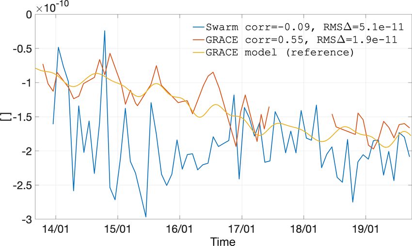
J. Teixeira da Encarnação et al.: Description of the gravity field models from Swarm GPS data                                                                          1389

Table 1. Overview of the kinematic orbits and the software packages used to estimate them.

            Institute     Software                                                                                    Reference
            AIUB          Bernese v5.3 (Dach et al., 2015; Jäggi et al., 2006)                                        Jäggi et al. (2016)1
            IfG           Gravity Recovery Object Oriented Programming System (GROOPS)                                Zehentner and Mayer-Gürr (2016)2
                          (in-house development)
            TUD           GPS High precision Orbit determination Software Tool (GHOST)                                van den IJssel et al. (2015)3
                          (van Helleputte, 2004; Wermuth et al., 2010)
          1 ftp://ftp.aiub.unibe.ch/LEO_ORBITS/SWARM (last access: 5 June 2020). 2 ftp://ftp.tugraz.at/outgoing/ITSG/tvgogo/orbits/Swarm (last access: 5 June 2020).
          3 http://earth.esa.int/web/guest/swarm/data-access (last access: 5 June 2020).

Table 2. Overview of the kinematic baselines and the software packages used to estimate them.

      Institute    Software                                                                                                                Reference
      AIUB         Bernese v5.3 (Dach et al., 2015)                                                                                        Jäggi et al. (2007, 2009)
      TUD          Multiple-satellite orbit determination using Kalman filtering (MODK) (van Barneveld, 2012)                              Mao et al. (2018)

2.3     Non-gravitational accelerations                                                      For the TUD model, the Near Real-Time Density Model
                                                                                          (NRTDM) software was employed (Doornbos et al., 2014).
We assessed the quality of the Swarm GFMs when the non-                                   This software, as part of the “official” Swarm Level 2 Pro-
gravitational accelerations are modelled following two dis-                               cessing System (L2PS) infrastructure, is used in the L1B to
tinct approaches and when they are represented by the Level                               Level 2 (L2) processing at TUD. A variety of models and pa-
1B (L1B) accelerometer data from Swarm C (Siemes et al.,                                  rameters related to the non-gravitational forces are available
2016). One non-gravitational acceleration model was pro-                                  in this software. For the current study, the following selection
duced at the Astronomical Institute Ondřejov (ASU) and the                               was made.
other at the Delft University of Technology (TUD). We se-
lected a number of periods for our tests (see Table 3), tak-                                  – The Swarm panel model (macromodel) is based on
ing care to cover as much as possible different accelerometer                                   Siemes (2019).
data variability (arising from instrument artefacts) and sig-
nal amplitude, as well as ionosphere and geomagnetic activ-                                   – The panel orientation is dictated by Swarm quaternion
ity, to cover different regimes of non-gravitational accelera-                                  data.
tions acting on the Swarm satellites. Moreover, we also chose
                                                                                              – The satellite aerodynamics of single-sided flat panels
months when GRACE gravity field solutions are available, to
                                                                                                are computed following Sentman’s equations (Sentman,
facilitate validation of the Swarm GFMs.
                                                                                                1961), assuming diffuse reflection and energy flux ac-
   For the ASU model, we used the in-house orbital propa-
                                                                                                commodation set at 0.93.
gator NUMINTSAT (Bezdek et al., 2009) for processing the
satellite orbital data, computing the coordinate transforma-                                  – The neutral densities are derived from the NRLMSISE
tions and generating the modelled non-gravitational acceler-                                    thermosphere model, as well as temperature and com-
ations of each Swarm satellite. The computation of the non-                                     position dependence of Sentman’s equations.
gravitational acceleration forces requires the knowledge of
the physical properties of the satellite based on the informa-                                – The velocity of the atmosphere with respect to the
tion provided by the ESA: its mass, cross section in a specific                                 spacecraft is based on the orbit and attitude data, atmo-
direction, radiation properties of the satellite’s surface, and a                               spheric co-rotation, and modelled thermospheric wind
macromodel characterizing approximately the shape of the                                        using the Horizontal Wind Model 07 (HWM07) (Drob
Swarm satellites. For neutral atmospheric density, we made                                      et al., 2008) and the Disturbance Wind Model 07
use of the US Naval Research Laboratory Mass Spectrome-                                         (DWM07) (Emmert et al., 2008).
ter and Incoherent Scatter Radar (NRLMSISE) atmospheric
model (Picone et al., 2002). We estimated the drag coeffi-                                    – The solar radiation pressure (SRP) is computed taking
cient of each satellite by means of the long-term change in                                     into account absorption, diffuse reflection, and specular
the orbital elements in order to consider realistic values. Fur-                                reflection, according to optical properties of the surface
ther details of our approach can be found in Bezdek (2010)                                      materials supplied by ESA and Astrium, and it consid-
and Bezdek et al. (2014, 2016, 2017).                                                           ers the varying Sun-satellite distance.

https://doi.org/10.5194/essd-12-1385-2020                                                                      Earth Syst. Sci. Data, 12, 1385–1417, 2020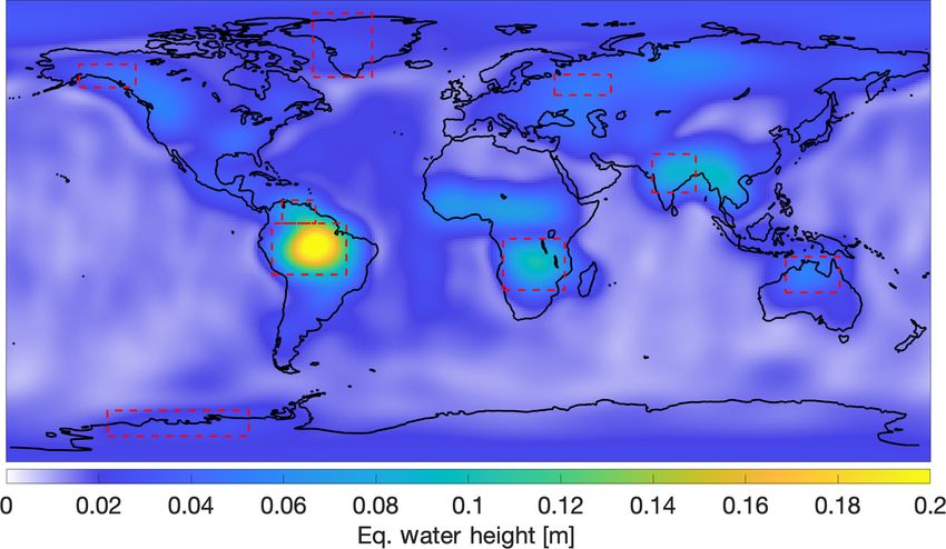
1390                           J. Teixeira da Encarnação et al.: Description of the gravity field models from Swarm GPS data

Table 3. Periods considered in the analysis of the added value of different types of non-gravitational accelerations.

                                              Accelerometer      Ionospheric      Geomagnetic    Accelerometer
                           Period             artefact density   activity         activity       signal magnitude
                           January 2015       high               high             low            high
                           February 2015      middle             middle           low            high
                           March 2015         low                high             high           high
                           January 2016       middle             low              low            low
                           February 2016      middle             low              low            low
                           March 2016         low                low              low            low

Table 4. Overview of the gravity field estimation approaches.

               Inst.    Approach                                                            Reference
               AIUB     Celestial mechanics approach (Beutler et al., 2010)                 Jäggi et al. (2016)
               ASU      Decorrelated acceleration approach (Bezdek et al., 2014, 2016)      Bezdek et al. (2016)
               IfG      Short-arc approach (Mayer-Gürr, 2006)                               Zehentner and Mayer-Gürr (2016)
               OSU      Improved energy balance approach (Shang et al., 2015)               Guo et al. (2015)

  – The Sun–Earth eclipse model takes into account atmo-                  GPS measurements is corrected for location of the GPS an-
    spheric absorption and refraction, according to the anal-             tenna phase centre with the L1B Swarm attitude data. The
    ysis of non-gravitational accelerations due to radiation              KOs are suitable to gravimetric studies due to their purely ge-
    pressure and aerodynamics (ANGARA) implementa-                        ometric nature. Through a parameter estimation procedure,
    tion (Fritsche et al., 1998).                                         i.e. one of the strategies listed in Table 4, the gravity field pa-
                                                                          rameters are derived from a functional relationship between
  – The Earth infrared radiation pressure (EIRP) and Earth                the kinematic positions and gravity field parameters. Com-
    albedo radiation pressure (EARP) are based on the AN-                 plementary to the KOs, numerous processing choices are
    GARA implementation.                                                  made by the four gravity field ACs, as enumerated in Ap-
                                                                          pendix C.
  – The monthly average albedo coefficients and infrared
                                                                             Each AC selects one KO solution to produce their so-
    radiation (IR) irradiances are derived from the Earth
                                                                          called individual GFMs, as listed in Table 4. In contrast, the
    Radiation Budget Experiment (ERBE) data (Barkstrom
                                                                          combined GFMs are derived from these individual solutions,
    and Smith, 1986).
                                                                          as discussed in Sect. 2.5. The following subsections provide
The equations for the algorithms and references for these                 a brief recap of the selected methods. Elaborate details can
models are available in Doornbos (2012) with updates spe-                 be found in the cited literature.
cific to Swarm provided by Siemes et al. (2016).
   For the Swarm C accelerometer data, we took advantage                  2.4.1     Celestial mechanics approach
of the corrected L1B along-track accelerometer data (Siemes
                                                                          The celestial mechanics approach (Beutler et al., 2010), used
et al., 2016), which are distributed by ESA and processed
                                                                          at AIUB, is a variation in the traditional variational equations
in a single batch from July 2014 to April 2016. We ap-
                                                                          approach (Reigber, 1989), which linearizes the relation be-
plied a dedicated calibration method to the Level 1A (L1A)
                                                                          tween the kinematic positions and the unknown Stokes coef-
product ACCxSCI_1A for the cross-track and radial compo-
                                                                          ficients as well as other unknown parameters that play a role
nents (Bezdek et al., 2017, 2018b), but, as shown by Bezdek
                                                                          in the dynamic model described by the equations of motion,
et al. (2018a), this approach was unable to recover the ex-
                                                                          such as initial state vectors, empirical accelerations, drag co-
pected signal. For this reason, the non-gravitational accelera-
                                                                          efficients, and instrument calibration parameters (possibly)
tion measurements are restricted to the available along-track
                                                                          amongst others. Pseudostochastic pulses or accelerations are
Swarm C data.
                                                                          estimated to mitigate deficiencies of the a priori force model.
                                                                          The CMA has successfully been applied for gravity field de-
2.4    Gravity field model estimation approaches                          termination from a number of LEO satellites, e.g. Meyer et
The estimation of the hl-SST GFMs takes the KOs as obser-                 al. (2019b).
vations, which describe the satellite’s centre of mass (CoM)
motion since in their production the processing of the L1B

Earth Syst. Sci. Data, 12, 1385–1417, 2020                                                 https://doi.org/10.5194/essd-12-1385-2020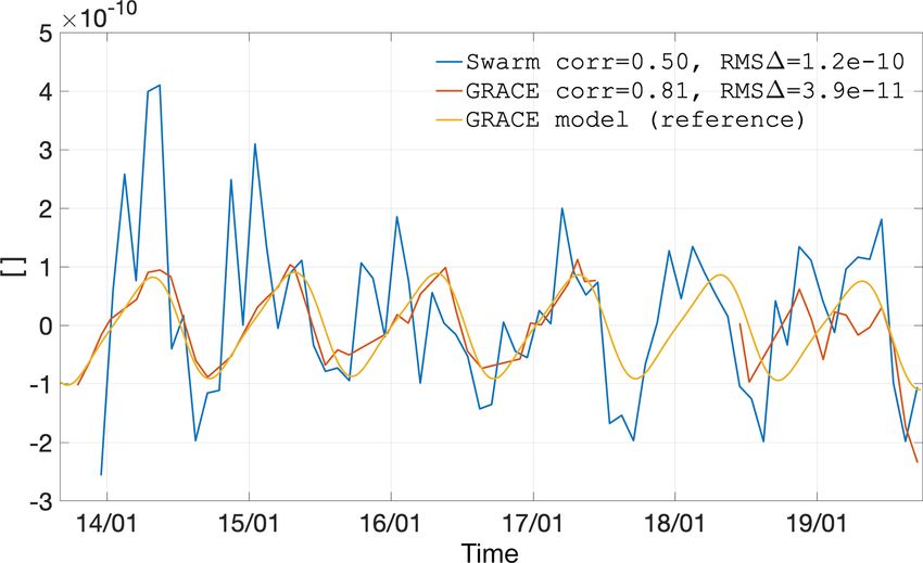
J. Teixeira da Encarnação et al.: Description of the gravity field models from Swarm GPS data                                 1391

2.4.2   Decorrelated acceleration approach                        and the kinematic positions as the boundary value problem
                                                                  resulting from the double integration of the equations of mo-
The decorrelated acceleration approach (DAA) (Bezdek
                                                                  tion. This approach naturally defines the initial state vector as
et al., 2014, 2016) used at ASU connects the double-
                                                                  the boundary conditions of the integral equation, which are
differentiated kinematic positions to the external forces act-
                                                                  regarded as unknowns in the LS estimation along with the
ing on the satellite. This approach computes the geopoten-
                                                                  Stokes coefficients and other unknown parameters, such as
tial harmonic coefficients from a linear (not linearized) sys-
                                                                  empirical parameters. Additionally, the kinematic positions
tem of equations. The observations are first transformed to
                                                                  are treated with no explicit differentiation, thus circumvent-
the inertial reference frame before differentiation to avoid
                                                                  ing the need to suppress the amplification of high-frequency
the computation of fictitious accelerations. The differentia-
                                                                  noise.
tion of noisy observations leads to the amplification of the
high-frequency noise. However, it is possible to mitigate the
high-frequency noise with a decorrelation procedure. We ap-       2.5   Combination
ply a second decorrelation based on a fitted autoregressive
                                                                  The individual GFMs are combined in the frame of the Com-
process to take into account the error correlations of the KOs.
                                                                  bination Service of Time-variable Gravity Fields (COST-G)
                                                                  of the IGFS, applying the methods developed during the
2.4.3   Improved energy balance approach                          EGSIEM project (Jäggi et al., 2019). We derive VCE weights
The traditional energy balance approach (EBA) exploits the        in order to produce the combined GFMs from the individual
energy conservation principle to build a relation between the     GFMs produced at AIUB, ASU, IfG, and OSU. The VCE
residual geopotential coefficients (relative to the reference     weights are derived at the solution level according to Jean et
background force model) and the deviations of the KO from         al. (2018), considering the individual models up to degree 20
the reference orbit on (Jekeli, 1999; Visser et al., 2003; Guo    only; if this is not done, the extremely high noise at the de-
et al., 2015; Zeng et al., 2015). The main development of         grees close to 40 (the maximum degree of the individual so-
the IEBA, used at The Ohio State University (OSU), con-           lutions) dominates the estimation of the weights, which leads
cerns the handling of the noise in the kinematic position and     to a slightly worse agreement with GRACE (Teixeira da En-
the weighting of the potential observations. Unlike the appli-    carnação and Visser, 2019). Irrespective of this, the maxi-
cation of this approach to GRACE ll-SST data by Shang et          mum degree of the combined models is the same as that of
al. (2015), the term related to the Earth’s rotation cannot be    the individual models (degree 40). We also tested the combi-
neglected in the processing of hl-SST data. From the kine-        nation at the level of normal equations (NEQs) (Meyer et al.,
matic positions, the velocity is derived with 61 data points,     2019a) but determined that the signal content was not in as
a sliding window, and quadratic polynomial filter similar to      good agreement with GRACE as the combination at the level
Bezdek et al. (2014). The polynomial coefficients of the filter   of solutions with weights derived from VCE (Teixeira da En-
are estimated in a LS adjustment, with the observation vector     carnação and Visser, 2019; Meyer, 2020). We attributed this
being composed of position residuals between the kinematic        result to the difficulty in calibrating the formal error types re-
positions and the corresponding reduced-dynamic positions         sulting from the different gravity field estimation techniques.
(integrated on the basis of the reference background force        There is the issue of the different types of error: some pro-
model), and the observation covariance matrix constructed         vide calibrated errors (e.g. DAA), while others provide the
from the epoch-wise variance–covariance information dis-          formal errors from the LS estimates (e.g. CMA). Another is-
tributed in the KO data files. As a consequence of this orbit     sue is the different error amplitude dependence with degree,
smoothing procedure, we discard the warm-up–cool-down             thus preventing the errors from being calibrated with a sim-
edges of the daily data arcs. We further remove one cycle         ple bias. Finally, the time-dependent levels of errors in the
per revolution (CPR) sinusoidal and 3-hourly quadratic poly-      individual models, which change their fidelity with time, and
nomial signals from the potential observations derived from       consequentially their optimum relative weights, were also a
the smooth kinematic positions. We also take advantage of         factor preventing us from successfully performing a combi-
the observation covariance matrix to weight the filtered kine-    nation at the NEQ level.
matic observations in the geopotential coefficient LS inver-
sion. We do not apply any a priori constraints nor iterate the    2.6   Assumptions in the gravity field model analyses
LS estimation since we take advantage of the linear relation
between the potential observations and the geopotential co-       This section describes the set of assumptions considered in
efficients.                                                       the analysis done in Sect. 3.3 and 3.4. Section 3.1 and 3.2 re-
                                                                  port parallel studies that were conducted with different back-
                                                                  ground force models, better suited to their respective pur-
2.4.4   Short-arc approach
                                                                  poses.
The short-arc approach (Mayer-Gürr, 2006), used at IfG, for-         We have chosen the release 6 (RL06) GRACE and
mulates the relation between the geopotential coefficients        GRACE-FO GFMs produced at the Center for Space Re-

https://doi.org/10.5194/essd-12-1385-2020                                         Earth Syst. Sci. Data, 12, 1385–1417, 2020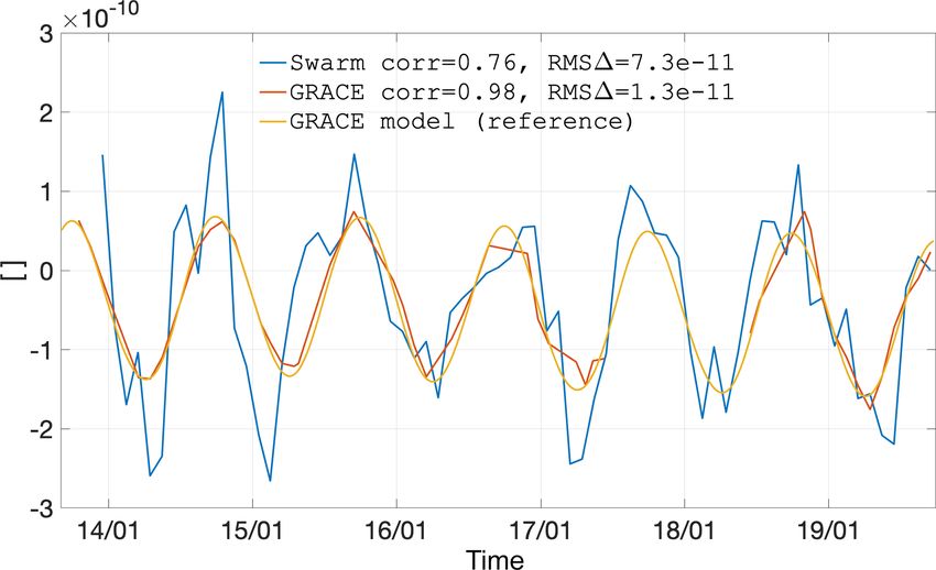
1392 J. Teixeira da Encarnação et al.: Description of the gravity field models from Swarm GPS data
search (CSR) as comparison in our analysis of the Swarm
GFMs. At the spatial scales relevant to Swarm, we have no
reason to expect our results would change significantly if
GRACE data produced at any other AC were used instead.
Unless otherwise noted, we apply a 750 km radius Gaus-
sian smoothing, which we motivate in Sect. 3.4.1, to isolate
the signal content in the Swarm models. The geo-centre mo-
tion has been ignored in our analysis, i.e. the degree 1 co-
efficients are always zero. The Combined GRACE Gravity
Model 05 (GGM05C) static GFM (Ries et al., 2016) is sub-
tracted from all Swarm and GRACE solutions in order to iso-
late the time-variable component of Earth’s gravity field. The Figure 1. Deep-ocean mask shown as dark areas.
gravity field is presented in terms of equivalent water height
(EWH), except for the statistics related to the correlation co-
efficient or when presenting coefficient-wise time series. it purely under the consideration it was the most technically
We consider the entirety of the Swarm GFM time series, convenient option for our needs.
irrespective of the epoch-wise quality because our objective
is to give a complete overview of the quality and character- 2.6.2 Deep-ocean areas
istics of our models. The analysis spans all available months
during the Swarm mission, i.e. between December 2013 and We consider the ocean mask of the areas away from conti-
September 2019. When comparing Swarm and GRACE di- nental masses illustrated in Fig. 1. To produce this mask, we
rectly, the Swarm time series is linearly interpolated to the start with a grid with a unit value over land areas, convert
time domain defined by the epoch of the GRACE solutions, it to the spherical harmonic (SH) domain, apply Gaussian
except for the GRACE-to-GRACE-FO gap, where no inter- smoothing with a radius of 1000 km, convert it back to the
polation is performed. We detrend the time series of models spatial domain, and define those grid points with values be-
at the level of the Stokes coefficients when computing non- low the cut-off value of 0.9 to be in deep-ocean areas. The
linear statistics, notably the epoch-wise spatial rms in Figs. 6, cut-off value was selected on the basis of trial and error with
9, 10, 11, 13, and 16. the objective of generating an ocean mask with the desired
and arbitrary buffer lengths, which for the results reported
here remained equal to 1000 km. This procedure pushes the
2.6.1 Earth’s oblateness
boundary of an ocean mask away from continental coastal ar-
In our analysis, the proper handling of Earth’s oblateness is eas and ignores islands. For the spatial scales relevant to the
not a trivial problem. In the case of GRACE, the mass esti- Swarm GFMs, we propose that this procedure is adequate.
mates are improved if C2,0 is augmented with satellite laser
ranging (SLR) data, which are provided in the form of the 2.6.3 GRACE climatological model
time series produced by Cheng and Ries (2018). Therefore,
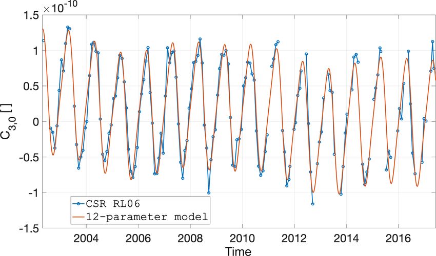
any comparison with mass variations derived from Swarm In the analyses conducted in Sect. 3.5.1, where we present
must also have the C2,0 coefficient replaced by the same time the time series of selected Stokes coefficients, we use a para-
series. One could argue that simply discarding this coefficient metric representation of Earth’s temporal mass changes as
would suffice for any comparison but we also intend to repre- observed by GRACE, which we refer to as the climatologi-
sent the actual mass changes observed by Swarm, notably in cal model since it captures mass variations that are present
Sect. 3.5.3, where we show mass variations over large storage in all 15 years of GRACE data. We do not use any GRACE-
basins. Unfortunately, Earth’s oblateness estimates provided FO data in this regression, in order to be able to verify the
by Cheng and Ries (2018) are exclusively available at those continuity of the GRACE-FO data, relative to GRACE and
epochs when there are GRACE solutions. That essentially to substantiate any deviation that is also observed by Swarm.
means that interpolating these GRACE–SLR C2,0 estimates This parametric regression is performed on the original CSR
over large gaps would lead to unrealistic mass variations. RL06 models, i.e. before any smoothing or masking.
For this reason, we selected the C2,0 weekly time series We selected the first-order polynomial to represent bias
from Loomis et al. (2019), since the necessary interpolation and trend in the GRACE data. For the periodic parameters,
introduces negligible deviations. We are not advocating that we choose the year and semi-year periods since these are
the considered C2,0 time series is in any way superior to dominant signals in the GRACE and Swarm data. We also
other solutions, e.g. those of Cheng et al. (2011) (which is modelled the S2, K2, and K1 tidal periods, with durations
only available at the middle of calendar months) or Cheng of 0.44, 3.83, and 7.67 years, respectively. These periods are
and Ries (2018) (which is only available for epochs compat- driven by the orbital inclination of the GRACE satellites and
ible with the GRACE monthly solutions); we have selected produce strong aliasing in the GFM time series (Ray and
Earth Syst. Sci. Data, 12, 1385–1417, 2020 https://doi.org/10.5194/essd-12-1385-2020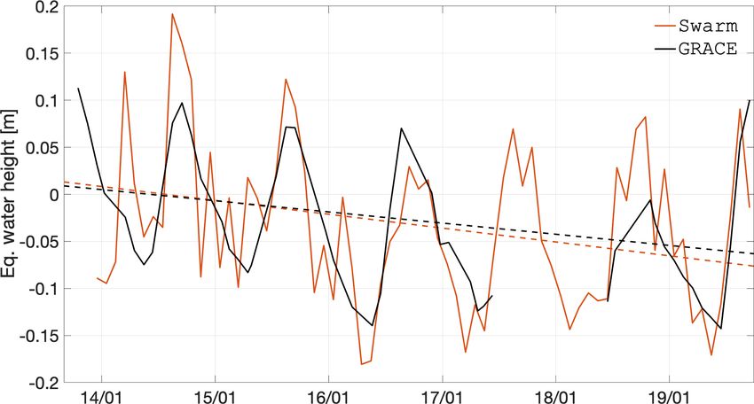
J. Teixeira da Encarnação et al.: Description of the gravity field models from Swarm GPS data                                 1393

                                                                    3.1   Kinematic baselines

                                                                    This section is dedicated to quantifying the benefit of exploit-
                                                                    ing KBs in the quality of the GFMs derived from Swarm
                                                                    data, following the motivation and procedures described in
                                                                    Sect. 2.2.
                                                                       Due to the decreasing ionospheric activity and the changes
                                                                    made to the Swarm on-board GPS receivers between 2015
                                                                    and 2016 (van den IJssel et al., 2016), the consistency of the
                                                                    KB solutions has improved. Especially in summer 2016, the
                                                                    overall daily SD of the difference between the reduced dy-
                                                                    namic ambiguity-fixed and kinematic ambiguity-fixed base-
                                                                    lines may be as low as 10–15, 4–6, and 3–5 mm on average
Figure 2. Agreement between the GRACE climatological model
                                                                    for the radial, along-track, and cross-track directions, respec-
and the GRACE data, exemplified by the C3,0 coefficient.
                                                                    tively, while it is as high as 1–3 cm for 2015 in all three di-
                                                                    rections. It should be noted, however, that daily SD is always
Luthcke, 2006; Cheng and Ries, 2017). The linear regres-            dominated by the low-quality kinematic positions over the
sion of the 12 parameters is done independently for each SH         polar regions. Eliminating such problematic data, the differ-
coefficient, up to degree 40 (in agreement with the maxi-           ence SD is consistently under 5 mm; therefore, the internal
mum degree of the Swarm models). This results in 12 sets            precision of the Swarm GPS data is of very good quality.
of Stokes coefficients, one for each of the model parame-              Figure 3 shows the degree amplitudes with respect to
ters: bias, trend, and five periods represented by their sine       the static part of the GOCO release 05 satellite-only grav-
and co-sine components. Each set of parametric Stokes co-           ity field model (GOCO05S) (Mayer-Gürr, 2015) in terms of
efficients has an implicit time dependence which is evalu-          geoid heights, representative of the results for bad, interme-
ated coefficient-wise at the epochs of the Swarm GFMs. We           diate, and good data quality. For comparison the correspond-
illustrate the general agreement between the climatological         ing month from the ITSG GRACE-only model 2016 (ITSG-
model and the GRACE data for the case of C3,0 in Fig. 2.            Grace2016) time series is also shown. For all months it can
   We regard this model as a good representation of the Earth       be seen that the solutions do not differ significantly. There
system; it is by definition inferior to the original GRACE          are small differences between the two ACs (AIUB and TUD)
time series because it truncates the signal bandwidth to dis-       as well as between the hl-SST-only and the ll-SST + hl-SST
crete frequencies. In spite of this, the assumed climatological     solutions. Differences are larger for those months with bad
model provides a measure to which both GRACE and Swarm              data quality (2015) and at the SH degree regions dominated
can be compared. The differences between GRACE and this             by noise (above degree 15), with the ll-SST and hl-SST so-
model should be regarded as the signal augmentation that            lutions showing larger degree amplitudes. For months with
GRACE brings, not as an error. We also regard the vastly            good data quality (June 2016) all four solutions display much
different spatial sensitivity of Swarm compared to GRACE            smaller differences.
as an additional argument that the climatological model is             To quantify the impact on the long-wavelength part of
able to represent the Earth system in a much more accurate          the solutions, we have compared the individual solutions to
way than Swarm, with the exception of large atypical mass           ITSG-Grace2016 monthly solutions in the spatial domain.
variations (which are uniquely revealed by Swarm).                  The solutions are evaluated on an equiangular grid (1◦ × 1◦ ),
                                                                    reduced by the corresponding ITSG-Grace2016 monthly so-
                                                                    lution, and filtered with a 500 km Gaussian filter, and finally
3   Results                                                         the rms over all grid cells is computed. The filter width was
                                                                    selected so as to avoid suppressing all of the signal at de-
Our results are shown in the following section, where we
                                                                    grees above 20 in order to assess the impact of KBs on the
analyse the added value of KBs in Sect. 3.1, look into the
                                                                    high-frequency noise as well. These results are summarized
effect of including accelerometer measurements of Swarm C
                                                                    in Table 5.
in Sect. 3.2, provide an overview of the quality of our indi-
                                                                       Table 5 confirms what is depicted in Fig. 3; i.e. the in-
vidual solutions in Sect. 3.3, quantify the quality of the com-
                                                                    clusion of KBs in the gravity field estimation has no signif-
bined solutions in Sect. 3.4, and illustrate their signal content
                                                                    icant impact on the quality of the resulting GFM. KO-only
in Sect. 3.5.
                                                                    solutions are already of very similar quality when compared
                                                                    to KB-augmented solutions, with small differences visible
                                                                    in the degree amplitude plots or the spatial rms having no
                                                                    discernible correlation with the data period (and therefore
                                                                    quality). In general, this confirms the findings of Jäggi et

https://doi.org/10.5194/essd-12-1385-2020                                          Earth Syst. Sci. Data, 12, 1385–1417, 2020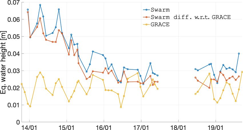
1394                         J. Teixeira da Encarnação et al.: Description of the gravity field models from Swarm GPS data

Table 5. Rms of geoid height differences in millimetres for different hl-SST-only results and the ll-SST and hl-SST Swarm solutions with
respect to the corresponding ITSG-Grace2016 monthly solution.

                                                                         TUD                AIUN
                               Data quality   Solution                    ll-SST +              ll-SST +
                                                                hl-SST       hl-SST   hl-SST       hl-SST
                               Bad            January 2015         9.5          9.6       9.8       10.5
                                              March 2015          10.9         11.1       8.4        9.6
                               Intermediate   February 2016        7.5          7.4       7.4        7.2
                                              March 2016           8.8          8.6       7.3        7.3
                               Good           June 2016            5.4          5.5       4.8        4.8
                                              July 2016            6.7          6.5       6.3        6.1
                                              August 2016          5.7          5.8       5.3        5.4

al. (2009), in that there are some small benefits for higher          Sect. 2.3. Figure 4 compares three single-satellite gravity
degrees when using KB; this was attributed to the elimina-            field solutions derived from Swarm C data, considering the
tion of errors common to both satellites by using DD obser-           three non-gravitational accelerations, for January 2015.
vations. Our results suggest that common errors are already              The SH degree difference amplitudes illustrate that the
mostly absent in the computation of the Swarm KOs. Thus               measured non-gravitational accelerations improve the agree-
we found no added value in including KBs for the quality of           ment of the lowest degrees of the Swarm C monthly solution
Swarm GFMs.                                                           with respect to the GOCO05S model (Mayer-Gürr, 2015),
   Our results contrast with those of Guo and Zhao (2019),            which includes a time-variable component. We tested this
who demonstrated a noticeable improvement when KBs are                comparison relative to the ITSG-Grace2016 monthly GFM
used in conjunction with KOs to derive GFMs from hl-SST               (Mayer-Gürr et al., 2016) and observed similar results (not
GRACE data. As the authors mention, their approach ben-               shown). The improvement at the lowest degrees in the Swarm
efits from the 3D KB information, thus essentially increas-           C model when using observed non-gravitational acceleration
ing by a factor of 3 the number of observations. Although             data is in accordance with what was reported by Klinger and
these components are most likely not completely indepen-              Mayer-Gürr (2016), relative to GRACE gravity field recov-
dent, they provide observations with crucial information that         ery.
is not available along the line-of-sight (LoS) component, in             In view of the lack of reliable measured non-gravitational
particular along the radial direction. We also note that the          accelerations in Swarm A and Swarm B, the three-satellite
geometry of the GRACE formation provides a much more                  Swarm GFM considers the ASU modelled non-gravitational
stable amplitude and attitude of resulting KBs, which may             accelerations for these satellites. For Swarm C, we consider
benefit the ambiguity fixing and, consequently, their over-           three cases where the non-gravitational accelerations are ei-
all quality. In the case of Swarm, the KBs are close to zero          ther measured or represented by TUD or ASU’s model. In
and flip their orientation by 180◦ at the poles. Additionally,        this way, we isolate the effect of the three types of non-
GRACE accelerometer data were used to represent the non-              gravitational acceleration data. The results for January 2015
gravitational accelerations, which is less straightforward for        are shown in Fig. 5, using ASU and TUD models and cali-
the Swarm satellites. These differences, i.e. 3D baselines,           brated accelerometer data.
stable baseline length, and inclusion of accelerometer data,             The three-satellite solutions that use modelled non-
suggest that they may be necessary conditions for a positive          gravitational accelerations in Swarm C are remarkably simi-
added value of KBs to the quality of hl-SST-only GFMs. Fi-            lar (see Fig. 5). In spite of this, note that using accelerometer
nally, we also point out that the improvements reported in            data improved the agreement to GOCO05S for degrees 2 and
Guo and Zhao (2019) are only above SH degree 10, where                4.
the errors start to become dominant, thus reducing the prac-             To gather a better overview of the added value of the three
tical added value of including baselines in the estimation of         types of non-gravitational accelerations, we derive the fol-
hl-SST-only GFMs.                                                     lowing model difference D, similar to rms:
                                                                            q
                                                                      D = median(1h)2 + MAD(|1h|)2 ,                                (1)
3.2    Non-gravitational accelerations
                                                                      with the median absolute deviation (MAD) analogous to SD
In this section, we present the inter-comparison of the               when the median is considered instead of the mean and
three types of non-gravitational accelerations described in           1h being the 1◦ × 1◦ geoid height difference between the

Earth Syst. Sci. Data, 12, 1385–1417, 2020                                             https://doi.org/10.5194/essd-12-1385-2020
J. Teixeira da Encarnação et al.: Description of the gravity field models from Swarm GPS data 1395
Figure 4. Swarm C gravity field solutions using TUD and ASU
modelled non-gravitational accelerations, as well as measured non-
gravitational accelerations (January 2015).
Table 6. Geoid height difference in millimetres between Swarm and
GRACE GFMs.
ITSG-Grace2016 GOCO05S
Mod. Mod. Mod. Mod.
ASU TUD Obs. ASU TUD Obs.
January 2015 16.2 15.6 15.0 16.7 16.5 15.9
February 2015 18.8 18.0 17.9 18.0 17.7 17.5
March 2015 16.4 16.5 16.1 16.2 16.3 16.0
January 2016 20.3 20.0 20.5 17.5 17.3 17.3
February 2016 23.9 22.3 25.6 15.2 14.3 16.3
March 2016 17.1 15.6 18.5 12.5 12.4 12.9
for January 2016 and GOCO05S, when the GFM derived
from TUD-modelled non-gravitational accelerations agrees
equally well with the one derived considering observed non-
gravitational accelerations). The comparison with GOCO05S
intends to predict how possible it would be to assess the
added value of the different types of non-gravitational ac-
celerations during those periods when there are no GRACE
Figure 3. Difference SH degree amplitudes of all four test solutions
data. Other time-dependent models were tested, but those
with respect to GOCO05S, for March 2015 (a), February 2016 (b),
and June 2016 (c), regarded as representative of bad, intermediate, do not agree as closely with GRACE monthly models (not
and good data quality, respectively. shown).
The statistics in Table 6 imply that observed non-
gravitational accelerations are only beneficial when the am-
plitude of the non-gravitational accelerations is larger than
500 km Gaussian filtering three-satellite Swarm models and what was observed in 2016. This is likely related to the de-
both ITSG-Grace2016 and GOCO05S, in the latitude band creasing level of solar activity, which is approaching the min-
85◦ from the Equator. We note that similar results were ob- imum of its 11-year cycle (expected to reach the minimum in
tained using the CSR RL05 GRACE monthly solutions (not 2019). Through the influence of the solar radiation on the at-
shown). The resulting differences are shown in Table 6. mospheric density and resulting atmospheric drag, the low
The 2015 results indicate that the observed non- level of solar activity has a direct impact on the accelerome-
gravitational accelerations improve the agreement between ter measurements. The closer to the solar cycle minimum, the
the three-satellite Swarm models and ITSG-Grace2016 and lower magnitude and variability of the accelerometer signal
GOCO05S, while that is not the case for 2016 (except are. Another factor may be a potential worse performance of
https://doi.org/10.5194/essd-12-1385-2020 Earth Syst. Sci. Data, 12, 1385–1417, 20201396 J. Teixeira da Encarnação et al.: Description of the gravity field models from Swarm GPS data
Figure 6. Time dependence between December 2013 and Septem-
ber 2019 of the epoch-wise cumulative degree amplitude (or global
spatial rms) of the individual Swarm solutions, CSR RL06 GRACE,
Figure 5. Three-satellite Swarm gravity field solutions using and their difference, considering 750 km smoothing.
TUD- and ASU-modelled non-gravitational accelerations, as well
as measured non-gravitational accelerations for Swarm C and ASU-
modelled non-gravitational accelerations for Swarm A and B (Jan-
uary 2015). The various individual solutions show different levels of
quality. Generally speaking, the solutions from AIUB, ASU,
and IfG cluster together as agreeing better with GRACE,
the accelerometer calibration procedure under low levels of with their dispersion narrowing down after 2016. This sug-
solar activity, resulting from the lower signal-to-noise ratio gests that these approaches suffer differently in conditions of
(SNR) in the accelerometer data. In other words, the noise high solar activity, with ASU’s models being the least sensi-
and (potentially) uncorrected artefacts in the accelerometer tive overall. Possibly, ASU’s efforts to minimize the ampli-
data of Swarm C are substantial enough to limit the useful- fication of the high frequencies when performing the double
ness of these data to gravimetric studies, except when the differentiation of the kinematic positions has the side effect
solar activity is high (as was the case in 2015) or when the of suppressing the negative effects of the high solar activity
satellites’ altitude decays in the future. Given these character- in the quality of the kinematic orbits. In contrast, OSU’s so-
istics and the continuing solar minimum, our Swarm models lution consistently has lower agreement with GRACE. The
are not processed considering Swarm C accelerometer obser- velocity measurements, which are needed for IEBA (as well
vations, but we plan to revisit this issue once the solar activity as any EBA-type approach), are to be derived from the kine-
increases. matic positions by differentiation (then squared to obtain ki-
netic energy). The tedious data filtering and processing to
3.3 Individual Swarm models approximate velocity errors is still imperfect, particularly in
light of the spurious jumps in most of the kinematic orbits
In this section we illustrate the quality of the individual even in the cases without the GPS tracking signal degrada-
Swarm solutions. As described in Sect. 2.6, we directly com- tion, e.g. from the southern Atlantic anomaly.
pare Swarm at the epochs defined by GRACE under 750 km Another way of analysing the agreement between the in-
radius Gaussian smoothing. dividual solutions and GRACE is to derive per-coefficient
Figure 6 shows a measure of the evolution of the quality statistics of their temporal variations. One such statistic is the
of the individual Swarm solutions over the complete Swarm coefficient-wise temporal rms of the difference between the
data period. We also plot the cumulative degree amplitude Swarm individual solutions and GRACE, thus producing a
of GRACE, to illustrate the global spatial amplitude of the set of Stokes coefficients that describes the variability of that
geophysical processes represented by these data. There is a difference; from this set we compute the mean over each de-
clear improvement in the agreement of Swarm with GRACE, gree to represent the general agreement at the corresponding
from rms differences as high as 40 cm geoid height in early spatial wavelengths. The results are summarized in Fig. 7,
2014, down to 10 cm and below since 2016. We attribute which quantifies the agreement of Swarm and the GRACE
this increase in quality to the decrease in solar activity and climatological model in the spectral domain. Note that for
to the upgrades in the Swarm GPS receivers between 2015 most individual solutions, the rms difference decreases with
and 2016 (van den IJssel et al., 2016; Dahle et al., 2017). As degree as a result of the Gaussian smoothing, without which
demonstrated in Sect. 3.4, the Swarm models contain large the curves would have a strong overall positive slope.
errors in the ocean areas, which dominate the global spatial The ranking of quality of the individual solutions changes
rms difference; over land areas, the agreement with GRACE with spatial wavelength; for example, although OSU’s solu-
is much better. tions are consistently worse than IfG’s as shown in Fig. 6,
Earth Syst. Sci. Data, 12, 1385–1417, 2020 https://doi.org/10.5194/essd-12-1385-2020You can also read


