Hydrographic fronts shape productivity, nitrogen fixation, and microbial community composition in the southern Indian Ocean and the Southern Ocean
←
→
Page content transcription
If your browser does not render page correctly, please read the page content below
Biogeosciences, 18, 3733–3749, 2021
https://doi.org/10.5194/bg-18-3733-2021
© Author(s) 2021. This work is distributed under
the Creative Commons Attribution 4.0 License.

Hydrographic fronts shape productivity, nitrogen fixation, and
microbial community composition in the southern Indian Ocean
and the Southern Ocean
Cora Hörstmann1,2 , Eric J. Raes3,4,1 , Pier Luigi Buttigieg5 , Claire Lo Monaco6 , Uwe John1,7 , and Anya M. Waite3,1
1 AlfredWegener Institute for Polar and Marine Science, Bremerhaven, Germany
2 Department of Life Sciences and Chemistry, Jacobs University, Bremen, Germany
3 Ocean Frontier Institute and Department of Oceanography, Dalhousie University, Halifax, NS, Canada
4 CSIRO Oceans and Atmosphere, Hobart, Tasmania, Australia
5 Helmholtz Metadata Collaboration, GEOMAR, Kiel, Germany
6 LOCEAN-IPSL, Sorbonne Université, Paris, France
7 Helmholtz Institute for Functional Marine Biodiversity, Oldenburg, Germany

Correspondence: Cora Hörstmann (cora.hoerstmann@awi.de)

Received: 24 February 2021 – Discussion started: 15 March 2021
Revised: 9 May 2021 – Accepted: 24 May 2021 – Published: 22 June 2021

Abstract. Biogeochemical cycling of carbon (C) and nitro-        physical oceanographic features, while microbial activity re-
gen (N) in the ocean depends on both the composition and         sponds more to chemical factors. We conclude that concomi-
activity of underlying biological communities and on abiotic     tant assessments of microbial diversity and activity are cen-
factors. The Southern Ocean is encircled by a series of strong   tral to understanding the dynamics and complex responses of
currents and fronts, providing a barrier to microbial disper-    microorganisms to a changing ocean environment.
sion into adjacent oligotrophic gyres. Our study region strad-
dles the boundary between the nutrient-rich Southern Ocean
and the adjacent oligotrophic gyre of the southern Indian
Ocean, providing an ideal region to study changes in micro-      1   Introduction
bial productivity. Here, we measured the impact of C and
N uptake on microbial community diversity, contextualized        The Southern Ocean (SO), in particular its sub-Antarctic
by hydrographic factors and local physico-chemical condi-        zone, is a major sink for atmospheric CO2 (Constable et
tions across the Southern Ocean and southern Indian Ocean.       al., 2014). The SO is separated from the Indian South Sub-
We observed that contrasting physico-chemical characteris-       tropical Gyre (ISSG) by the South Subtropical Convergence
tics led to unique microbial diversity patterns, with signifi-   province (SSTC), comprising the Subtropical Front (STF)
cant correlations between microbial alpha diversity and pri-     and the Subantarctic Front (SAF). The SSTC is a zone
mary productivity (PP). However, we detected no link be-         of deep mixing and thus elevated nutrient concentrations
tween specific PP (PP normalized by chlorophyll-a concen-        (Longhurst, 2007). Further, the SSTC has been shown to act
tration) and microbial alpha and beta diversity. Prokaryotic     as a transition zone both numerically and taxonomically for
alpha and beta diversity were correlated with biological N2      dominant populations of marine bacterioplankton (Baltar et
fixation, which is itself a prokaryotic process, and we de-      al., 2016).
tected measurable N2 fixation to 60◦ S. While regional water        In this dynamic context, a key driver of microbial produc-
masses have distinct microbial genetic fingerprints in both      tivity is nutrient availability, especially through tightly cou-
the eukaryotic and prokaryotic fractions, PP and N2 fixation     pled carbon (C) and nitrogen (N) cycles. The constant avail-
vary more gradually and regionally. This suggests that mi-       ability of nutrients through vertical mixing in frontal zones,
crobial phylogenetic diversity is more strongly bounded by       such as the STF, enhances primary productivity (Le Fèvre,

Published by Copernicus Publications on behalf of the European Geosciences Union.
3734                                             C. Hörstmann et al.: Microbial provincialism in the southern Indian Ocean

1987) and chlorophyll-a (chl a) concentrations (Belkin and                 often separate water masses with distinct trophic struc-
O’Reilly, 2009). Primary productivity (PP) and specific pri-               tures (e.g., Albuquerque et al., 2021).
mary productivity (P B , meaning primary productivity per
                                                                        3. Microbial alpha and beta diversity are impacted by N2
unit chl a) are reflected in the relative abundance of dif-
                                                                           fixation, which is itself correlated with the presence of
ferent phytoplankton size classes whose productivity values
                                                                           other available sources of N and/or temperature; this is
are, in turn, stimulated by nutrient injections via shallowing
                                                                           to provide more evidence on the role of N2 fixation to
of mixed layer depth (MLD) at the SO fronts (Strass et al.,
                                                                           the N budget in high latitudes (see e.g., Shiozaki et al.,
2002); decreasing the possibility of N limitation. However,
                                                                           2018; Sipler et al., 2017).
N limitation can also biologically be alleviated through N2
fixation mediated by diazotrophs, significantly contributing        To our knowledge, there are no concomitant evaluations of
to the N pool in oligotrophic regions (Tang et al., 2019).          how surface gradients, microbial activity, and community
In high-latitude regions, biological N2 fixation could poten-       composition relate to one another in this region. Here, we
tially have a large impact on productivity (Sipler et al., 2017).   provide perspectives on these key relationships across the In-
However, large disagreements exist between models of high-          dian South Subtropical Gyre (ISSG), the Subtropical Front
latitude N2 fixation and its coupling to microbial diversity        (STF), and Subantarctic Front (SAF), and the SO compris-
due to sparse sampling in these regions (Tang et al., 2019).        ing the Polar Front (PF) and Antarctic Zone (AZ).
   Due to the dynamics of the region, conflicting observa-
tions, and climate-driven changes, resolving the coupling of
microbial productivity and diversity is particularly important      2     Materials and methods
across the strong environmental gradients crossing the ISSG,
                                                                    2.1    Study region, background data, and sample
through the SSTC into the SO. Indeed, climate variability has
                                                                           collection
been shown to impact ocean productivity and thus influences
the provision of resources to sustain ocean life (Behrenfeld        Our study region ranged from Réunion in the Indian South
et al., 2006). To date, observations of climate-change-related      Subtropical Gyre (ISSG) to south of the Kerguelen Islands
effects in this region of the SO have been synthesized only         in the Southern Ocean (56.5◦ S, 63.0◦ E; Fig. 1a) as part of
based on long-term nutrient concentration and physical (tem-        a larger repeated “OISO” sampling program – (Océan In-
perature and salinity) changes (Lo Monaco et al., 2010);            dien Service d’Observations; Metzl and Lo Monaco, 1998;
however, these typically lack a microbial dimension. Micro-         https://doi.org/10.17600/17009700). Samples were collected
bial composition, activity, and C export may all be impacted        as part of the VT153/OISO27 (MD206) cruise aboard the
by climate-driven changes in ocean dynamics (Evans et al.,          R/V Marion Dufresne from 6 January to 7 February 2017.
2011) such as MLD shallowing, eddy formation, and pole-             Physical and biogeochemical data, as well as metadata, were
ward shifts of ocean fronts (Chapman et al., 2020). For a           collected from a rosette equipped with Niskin bottles and
more holistic ecosystem-based understanding of this region,         a conductivity, temperature, depth sensor (CTD) (Sea-Bird
concomitant assessments of (1) steady-state biogeochemical          SBE32) equipped with a SBE43 O2 sensor and a Chelsea
processes through rate measurements of key elements (such           Aqua tracker fluorometer. OISO long-term data, starting in
as C and N) and (2) the microbial diversity that underpins it       1998, were used as a backdrop to our data collected in 2018
are essential enhancements to such long-term investigations.        and allowed us to monitor changes in physical and chemical
   Here, we measure the impact of C and N uptake on micro-          oceanographic properties over time (Supplement File A).
bial community diversity, alongside the effects of hydrog-
raphy (e.g., dispersal limitation) and local physico-chemical       2.2    Province delineation after Longhurst
conditions across the Southern Ocean and southern Indian
Ocean. We focused our investigation on surface communi-             We identified three main clusters (i.e., ocean provinces) and
ties, aiming to resolve horizontal surface variation. We used       five subclusters (i.e., water masses) on a temperature–salinity
our observation to assess whether the following relationships       plot (Fig. 1b). As an overview, we used CTD depth profiles
– previously observed in related systems – hold in our study        to validate the vertical extent of water masses in our samples
region:                                                             (Fig. 1c, d) and checked the horizontal extent of the identified
                                                                    clusters using remote sensing data of sea surface temperature
  1. Microbial diversity increases with increasing primary
                                                                    (Fig. S2 in the Supplement). Additionally, we checked the
     productivity (PP). Previous work has claimed that more
                                                                    horizontal boundaries of these clusters for matches in strong
     resources support higher species richness until interme-
                                                                    chl a concentration gradients as an approximate for biologi-
     diate rates of PP (Fig. 1; Vallina et al., 2014) within
                                                                    cal component of ocean provinces, following the concept of
     ocean provinces (Raes et al., 2018).
                                                                    Longhurst (2007). Satellite data were acquired from MODIS
  2. Frontal systems are discrete ecological transition zones       (https://neo.sci.gsfc.nasa.gov/, last access: 16 June 2021),
     between regions that provide perspectives on the find-         with images processed by NASA Earth Observations (NEO)
     ings of Baltar et al. (2016; see above). These systems         in collaboration with Gene Feldman and Norman Kuring,

Biogeosciences, 18, 3733–3749, 2021                                                     https://doi.org/10.5194/bg-18-3733-2021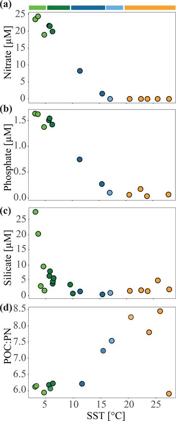
C. Hörstmann et al.: Microbial provincialism in the southern Indian Ocean                                                                   3735

Figure 1. (a) The MD206 transect and OISO stations. Stations are colored according to water masses and encircled by sampling extent:
black circles indicate stations where only CTD (conductivity, temperature, depth) data are provided, and stations encircled in red denote
where additional samples for C, N, and community composition were taken. (b) A plot of potential temperature (in degrees Celsius (◦ C) and
salinity (in practical salinity units)) using sea surface (7 m) data of the stations used in further microbial and C/N analyses. The yellow circle
highlights the Indian South Subtropical Gyre (ISSG), light blue circle the Subtropical Front (STF), blue circle the Subantarctic Front (SAF),
dark green circle the Polar Front Zone (PFZ) and the light green circle indicates the Antarctic Zone (AZ); dashed lines indicate water masses
clustered within ocean provinces: the blue line marks the South Subtropical Convergence province (SSTC), and the green line marks the
Southern Ocean (SO); panels (c) and (d) show depth profiles of temperature, oxygen, and salinity along two transects of the OISO stations.
Colored bars indicate water masses according to (b). Panel (c) shows the western transect covering OISO stations 2, 3, 4, 5, 6, and 37 around
53 ± 1◦ E longitude; panel (d) shows the eastern transect of OISO stations 10, 11, 12, 13, 14, 15, 16, and E around 68 ± 5◦ E.

i.e., NASA OceanColor Group (Fig. S3). We calculated the                   ods (Armstrong, 1951; Murphy and Riley, 1962; Wood et
geodesic distance between sites from latitude and longitude                al., 1967) with adaptations to particular needs for Seal An-
coordinates using the geodist package in R (v0.0.4; Padgham                alytical QuAAtro autoanalyzer. NH+   4 was measured using
et al., 2020).                                                             the fluorometric method of Kérouel and Aminot (1997).
                                                                           Detection limits of these methods were 0.1 µmol L−1 for
2.3   Nutrient analysis                                                    PO3−4 , 0.3 µmol L
                                                                                             −1 for Si, 0.03 µmol L−1 for NO , and
                                                                                                                                 x
                                                                           0.05 µmol L for NH+
                                                                                        −1
                                                                                                 4.
Dissolved inorganic nutrient concentrations, including phos-
phate (PO3−
          4 ), silicate (denoted Si), mono-nitrogen oxides
(NOx ), nitrite (NO−                           +
                    2 ), and ammonium (NH4 ), were as-
sayed on a QuAAtro39 continuous segmented flow analyzer
(Seal Analytical) following widely used colorimetric meth-

https://doi.org/10.5194/bg-18-3733-2021                                                              Biogeosciences, 18, 3733–3749, 2021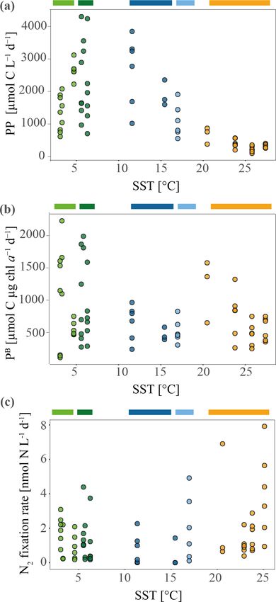
3736                                           C. Hörstmann et al.: Microbial provincialism in the southern Indian Ocean

2.4    Dissolved inorganic nitrogen and carbon                    2.5   Pigment analysis
       assimilation
                                                                  For pigment analyses, 4 L of seawater was filtered (< 10 kPa)
At each CTD station, water samples to measure primary pro-        on a 47 mm Whatman GF/F filter and stored at −80 ◦ C until
ductivity (PP) and N2 fixation were taken from the underway       further analysis. High-performance liquid chromatography
flow-through system (intake at 7 m). As the ship was mov-         (HPLC) was carried out as described in Kilias et al. (2013)
ing during sampling, the distance between samples of the          with the following modifications: 150 µL of the internal stan-
same station can range up to ∼ 15 km. Incubations were per-       dard canthaxanthin was included to each sample. Samples
formed in acid-washed polycarbonate bottles on deck at am-        were dissolved in 4 mL acetone and disrupted with glass
bient light conditions. All polycarbonate incubation bottles      beads using a Precellys 24 tissue homogenizer (Bertin Tech-
were rinsed prior to sampling with 10 % HCl (3×), deion-          nologies, France) at 7200 rpm for 20 s. Detection of the sam-
ized H2 O (3×), and sampling water (2×). In order to obtain       ple at 440 nm absorbance was performed using an HPLC an-
the natural abundance of particulate nitrogen (PN) and par-       alyzer (Varian Microsorb-MV 100-3 C8). We used chl a con-
ticulate organic carbon (POC), which we used as a t0 value        centration to estimate phytoplankton biomass. Pigment con-
to calculate the assimilation rates, 4 L of water was filtered    centrations were calculated according to Kilias et al. (2013)
onto a 25 mm pre-combusted GF/F filter for each station.          and quality controlled according to Aiken et al. (2009) (Sup-
   N2 fixation experiments were carried out in triplicate for     plement File A).
each station. We used the combination of the bubble ap-              HPLC output data were analyzed using diagnostic pig-
proach (Montoya et al., 1996) and the dissolution method          ments for the different taxa and phytoplankton functional
(Mohr et al., 2010) proposed by Klawonn et al. (2015). The        types (PFTs) after Hirata et al. (2011) (Supplement File A,
4.5 L bottles were filled up headspace free. All incubations      Table S2). This approach can be used to reveal dominant
were initialized by adding a 15 N2 gas bubble with a vol-         trends of the phytoplankton community and size structure at
ume of 10 mL. We used 15 N2 -labeled gas provided by Cam-         the regional and seasonal scales (Ras et al., 2008). Further-
bridge Isotope Laboratories (Tewksbury, MA). Bottles were         more, diagnostic pigments were used to delineate three dif-
gently rocked for 15 min. Finally, the remaining bubble was       ferent size classes (pico-, nano-, and microplankton) accord-
removed to avoid further equilibration between gas and the        ing to Vidussi et al. (2001). The relative proportion of each
aqueous phase. After 24 h, a water subsample was transferred      phytoplankton size class (PSC) was calculated based on the
to a 12 mL exetainer® and preserved with 100 µL HgCl2 so-         linear regression model proposed by Uitz et al. (2006). We
lution for later determination of exact 15 N–15 N concentra-      investigated the patterns of PSCs with a second-order poly-
tion in solution. Natural 15 N2 was determined using mem-         nomial fit (S1_code_archive/pigment_HPLC/diaganostic_
brane inlet mass spectrometry (MIMS; GAM200, IPI) for             pigments.R L143:153).
each station with an average enrichment of 3.8 ± 0.007 at. %
15 N (mean ± SD; n = 104). Primary productivity was mea-          2.6   DNA analysis
     2
sured by adding Na13 CO3 at a final 13 C concentration of
                                                                  Two liters of seawater from the shipboard underway system
200 µmol L−1 .
                                                                  from each station were filtered through a 0.22 µm Sterivex®
   Incubation bottles were incubated on board at ambient
                                                                  filter cartridge for DNA isolation, snap-frozen in liquid ni-
sea surface temperature (SST; water intake at 7 m) using
                                                                  trogen, and stored at −80 ◦ C. DNA was extracted using a
a continuous-flow-through system. Temperature of both in-
                                                                  DNeasy® Plant Mini Kit (QIAGEN, Valencia, CA, USA,
cubation bins was continuously measured. After 24 h, the
                                                                  catalog no. or ID 69106) following the manufacturer’s in-
C and N2 fixation experiments were terminated by collect-
                                                                  structions. Sterivex cartridges were gently cracked open, and
ing the suspended particles from each bottle by gentle vac-
                                                                  filters were removed and transferred into a new and ster-
uum filtration through a 25 mm pre-combusted GF/F filter
                                                                  ile screw-cap tube. Approximately 0.3 g of pre-combusted
(< 10 kPa). Filters were snap-frozen in liquid nitrogen and
                                                                  glass beads (diameter 0.1 mm; 11079101 Bio Spec Prod-
stored at −80 ◦ C while at sea. Filters with enriched (T24) and
                                                                  ucts) and 400 µL buffer AP1 were added to the filter, fol-
unenriched (T0) samples were acidified and dried overnight
                                                                  lowed by a bead beating step using a Precellys 24 tissue ho-
at 60 ◦ C. Analysis of 15 N and 13 C incorporated was carried
                                                                  mogenizer (Bertin Technologies, France), with two times at
out by the isotopic laboratory at the University of Califor-
                                                                  5500 rpm for 20 s with 2 min on ice in between and a final
nia, Davis, California campus, using an Elementar Vario EL
                                                                  bead beating step at 5000 rpm for 15 s. DNA concentrations
Cube or MICRO cube elemental analyzer (Elementar Analy-
                                                                  were quantified by the Quantus™ fluorometer and normal-
sensysteme GmbH, Hanau, Germany).
                                                                  ized to 2 ng µL−1 .
   Carbon assimilation rates were calculated according to
Knap et al. (1996), excluding the 14 C–12 C conversion fac-
tor, and N2 fixation was calculated according to Montoya et
al. (1996). The minimum quantifiable rate was calculated ac-
cording to Gradoville et al. (2017).

Biogeosciences, 18, 3733–3749, 2021                                                 https://doi.org/10.5194/bg-18-3733-2021
C. Hörstmann et al.: Microbial provincialism in the southern Indian Ocean 3737
2.6.1 Amplicon 16S and 18S rRNA gene PCR and S1_code_archive/import/import_18S.R L29). ASV tables
sequencing of 16S rRNA gene amplicon (Table S4) and 18S rRNA
gene amplicons (Table S5) were used for further statistical
Amplicons of the bacterial 16S rRNA gene and eukaryotic analyses.
18S rRNA gene (using primers from 27F–519R; Parada et
al., 2016, TA-Reuk454FWD1 – TAReukREV3; Stoeck et al., 2.7 Ecological data and statistical analysis
2010, respectively) were generated following standard proto-
cols of amplicon library preparation (16S Metagenomic Se- A combination of temperature, salinity, dissolved oxygen
quencing Library Preparation, Illumina, part no. 15044223 concentrations, and dissolved inorganic nutrient concentra-
3−
Rev. B; Supplement File B). The 16S and 18S rRNA gene tions (NO− − +
3 , NO2 , NH4 , Si, and PO4 ) were used to char-
PCR products were sequenced using 250 bp paired-end se- acterize the physical and biogeochemical environment of the
quencing with a MiSeq sequencer (Illumina) at the European study region.
Molecular Biology Laboratory (EMBL) in Heidelberg (Ger- All statistical tests were performed in R version 3.6.3 (R
many) and at the Leibniz Institute on Aging (FLI) in Jena Core Team, 2020). Statistical documentation, package cita-
(Germany), respectively. tions, and scripts are available in S1. Microbial alpha diver-
sity was calculated with Hill numbers (richness, Shannon en-
2.6.2 Amplicon sequence data analysis tropy, inverse Simpson, q = 0–2; Chao et al., 2014) using the
iNEXT package v2.0.20 in R with confidence set to 0.95 and
For both 16S rRNA gene and 18S rRNA gene ampli- bootstrap = 100 (S1_code_archive/alpha_diversity). Accord-
con sequences, we used the DADA2 R package, v1.15.1 ingly, rarefaction curves are shown in Fig. S6. Pearson cor-
(Callahan et al., 2016) to construct Amplicon sequence relations between microbial richness (q = 0), inverse Simp-
variant (ASV) tables by the following steps: prefiltering son diversity (q = 2), environmental parameters, and biolog-
“filterandtrim” function with truncL = 50 and default ical rates were calculated and plotted (ggplot2) (Fig. S7).
parameters (S1_code_archive/dada2). Primer sequences The p values were adjusted for multiple testing using Holm
were cut using the Cutadapt software implementation adjustment (Holm, 1979), and residuals were checked for
(v1.18) in the DADA2 pipeline, removing a fixed number normal distribution (Fig. S8). For comparability and statisti-
of bases matching the 16S forward (515F-Y, 19 bp) and cal downstream analyses, we performed the following trans-
reverse (926R, 20 bp) primers and the 18S forward (TA- formations to the ASV table and the environmental meta-
Reuk454FWD1, 20 bp) and reverse (TAReukREV3, 21 bp) data: to account for the compositionality of sequencing data
primers (S1_code_archive/dada2/dada2_16S.R L88:104; (see Gloor et al., 2017), we performed a centered log ra-
S1_code_archive/dada2/dada2_18S.R L92:104). Primer- tio (CLR)-transformation for redundancy analysis (RDA).
trimmed fastq files were quality trimmed with a minimum We used Hellinger transformation (decostand() function
sequence length of 50 bp and checked by inspection of in vegan) of the ASV pseudocount data (minimum pseudo-
the average sequence length distribution (for both the 16S count per ASV cutoff was 3) for PERMANOVA analyses.
rRNA gene and 18S rRNA gene sequences). Samples Environmental data were z scored for comparable metadata
within forward and reverse fastq files were dereplicated analysis (S1_code_archive/transformations). For multivari-
and merged with a minimum overlap of 20 bp. ASV tables ate analyses of microbial beta diversity and environmental
were constructed, and potential chimeras were identified parameters, we performed redundancy analyses (RDA) of
de novo and removed using the “removeBimeraDenovo” the CLR-transformed ASV tables (S1_code_archive/RDA).
command. Sequencing statistics for removed reads and Differences of microbial beta diversity (based on Hellinger-
sequences in each step can be found in Table S3. Tax- transformed ASV tables), phytoplankton community compo-
onomic assignment was performed using the SilvaNGS sition (based on pigment concentrations), and water masses
(v1.4; Quast et al., 2013) pipeline for 16S rRNA gene data were tested with permutational ANOVA (PERMANOVA;
with the similarity threshold set to 1. Reads were aligned Anderson, 2001) using the adonis2() function in vegan
using SINA v1.2.10 (Pruesse et al., 2012) and classified along with a beta dispersion test to evaluate the homogeneity
using BLASTn (v2.2.30; Camacho et al., 2009) with the of the dispersion (Fig. S9). To investigate where differences
Silva database (v132) as a reference database (Supplement of environmental variables have an impact on microbial com-
File C). For taxonomic assignment of 18S rRNA gene munity dissimilarity, we performed a general dissimilarity
amplicons, we used the plugin “feature-classifier” (from model (GDM) of the community dissimilarity and environ-
package “q2-feature-classifier”, v2019.7.0) in QIIME2 mental variables, and we checked for the influence of geo-
(Bokulich et al., 2018) and the pr2 database (v4.12; Guillou graphic distance based on spline magnitude (gdm package;
et al., 2013). We removed ASVs annotated to mitochondria S1_code_archive/GDM).
and chloroplasts from 16S rRNA gene ASV tables and As differences in microbial beta diversity were significant
ASVs annotated as metazoans from 18S rRNA gene ASV in PERMANOVA between provinces and water masses, we
tables (S1_code_archive/import/import_16S.R L35:38; performed a similarity percentage (SIMPER) analysis in R
https://doi.org/10.5194/bg-18-3733-2021 Biogeosciences, 18, 3733–3749, 20213738 C. Hörstmann et al.: Microbial provincialism in the southern Indian Ocean
using the vegan package to assess which ASVs contribute
most to the observed variance of microbial community com-
position (Table S6; S1_code_archive/taxonomy_analyses).
To determine the number of ASVs shared between provinces
(or unique to certain provinces), we transformed ASV pseu-
docount tables into binary tables and calculated shared and
unique ASVs using the upsetR package in R (v.4, Conway
et al., 2017; S1_code_archive/upsetR). We calculated the
percentage of all within-sample-observed ASVs within the
merged samples of a province (Table S7).
3 Results
3.1 Delimitation of regional water masses
Through our analysis of temperature, salinity, oxygen, and
dissolved inorganic nutrient (N, P, Si) concentrations, we
identified five distinct water masses, fronts, and frontal
zones: the ISSG, STF, SAF, PFZ, and AZ, which broadly
aligned with three oceanographic provinces (ISSG, SSTC,
and SO; Fig. 1a). Within the Southern Ocean (SO), we iden-
tified four water masses in our transect including the Antarc-
tic Zone (AZ) and three distinct frontal systems: (1) the Po-
lar Front (PF), (2) the Subantarctic Front (SAF), and (3) the
Subtropical Front (STF; Fig. 1). In our analysis, stations 6,
7, and 9 were placed within the Polar Front Zone (PFZ),
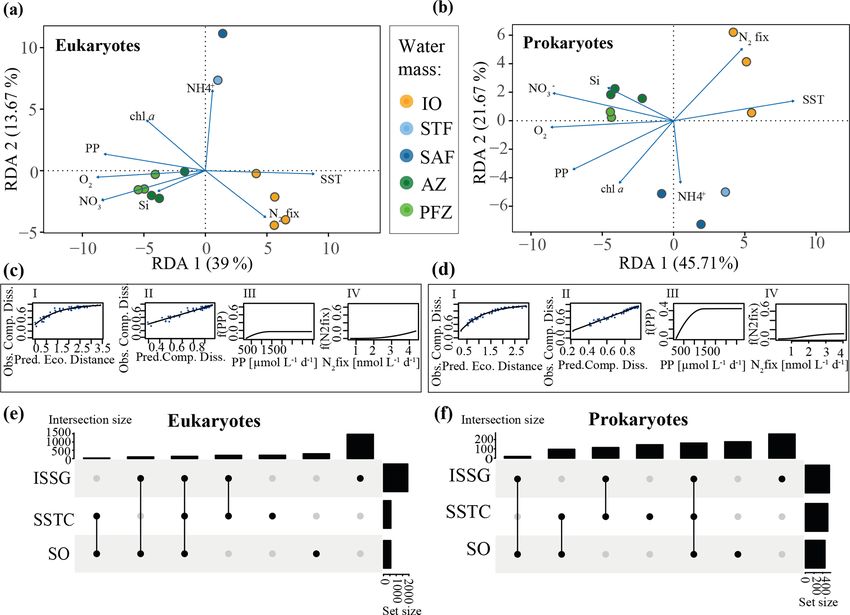
which is between the SAF and PF. Due to the bathymetri- Figure 2. Nutrient concentrations (µmol L−1 ) and molar ratios of
cally driven convergence of the STF and SAF around Ker- particulate organic carbon (POC) to particulate nitrogen (PN) dur-
guelen island, we consider the SAF as part of the conver- ing the MD206 expedition against sea surface temperature (◦ C):
gence zone between the SO and Indian Ocean (IO), i.e., (a) nitrate, (b) phosphate, (c) silicate, and (d) POC : PN ratio. Col-
the South Subtropical Convergence province (SSTC), rather ored bars indicate water masses according to their sea surface tem-
perature: yellow bar highlights the Indian South Subtropical Gyre
than as a Southern Ocean frontal system. At 7 m depth, we
(ISSG), light blue bar highlights the Subtropical Front (STF), blue
noted clear shifts in temperature (SST), salinity, and dis-
3− bar highlights the Subantarctic Front (SAF), dark green bar high-
solved inorganic nutrient (NO− 3 , PO4 , Si) concentrations lights the Polar Front Zone (PFZ), and light green bar highlights the
when crossing the STF. The STF is described as a circum- Antarctic Zone (AZ).
polar frontal zone creating the boundary between our mea-
surements of the warm (20–25 ◦ C), saline (> 35), and olig-
3−
otrophic (NO− 3 < 0.03 µM; PO4 : 0.04–0.21 µM) subtropical values (190.4–642.6 µmol C L−1 d−1 ) were measured at the
waters (STW) of the Indian South Subtropical Gyre (ISSG) stations in the Indian South Subtropical Gyre (ISSG). While
and the cold (3–6 ◦ C) macronutrient-rich SO (NO− 3 : 19.2– stations in the ISSG showed very little variations within
3−
24.9 µM; PO4 : 1.43–1.71 µM) (Figs. 1, 2, S3). In the con- one station (e.g., 226.09–371.07 µmol C L−1 d−1 , n = 6, sta-
text of this study, STW and ISSG could be used interchange- tion 18), variation within SO stations was relatively high
ably; we henceforth refer to it as ISSG. (e.g., 587.42–1875.58 µmol C L−1 d−1 , n = 6, station 37; Ta-
ble 1).
3.2 Primary productivity (PP) Overall, the variation of specific primary productivity
(P B ) did not show great variations between provinces, with
Maximum primary productivity (PP) values within our maximum rates at station 11 (Table 1; Fig. 3b). We did not
dataset were measured near the Kerguelen Plateau in find a significant correlation between mixed layer depth and
the Polar Front Zone (PFZ) at station 9 (3236.8 and P B (Pearson correlation: r = 0.21, p = 0.47, n = 12).
3553.3 µmol C L−1 d−1 , respectively) and station E (2212.4–
2688.1 µmol C L−1 d−1 , n = 6). Comparing all PP measure- 3.3 N2 fixation
ments across water masses, we found relatively high PP in
other stations of the PFZ (stations 6, 7; Fig. 3a; Table 1) and Di-nitrogen (N2 ) fixation was above the minimum quantifi-
in the Subantarctic Front (SAF) (stations 4, 15). Lowest PP able rate (MQR) at all stations (Table 1). N2 fixation mea-
Biogeosciences, 18, 3733–3749, 2021 https://doi.org/10.5194/bg-18-3733-2021C. Hörstmann et al.: Microbial provincialism in the southern Indian Ocean 3739
Table 1. Sampling stations visited during the MD206 cruise, including chlorophyll-a concentrations, primary productivity (PP), specific
primary productivity (P B ), and N2 fixation. Mixed layer depth (MLD) was calculated using 1d = 0.03 kg m−3 compared to a surface
reference depth of 7 m. NA indicates no data. Ranges and mean for sample replicates of N2 fixation and PP are given (n = 3 for stations 3,
9, 11, 15; n = 6 for stations E, 37, 2, 4, 6, 7, 14, 16, 18).
Station Latitude Longitude MLD chl a Primary productivity (PP) Specific PP (P B ) N2 fixation MQR
◦S ◦E [m] [µg L−1 ] [µmol C L−1 d−1 ] [µmol C µg chl a −1 L−1 d−1 ] [nmol N L−1 d−1 ] [nmol N L−1 d−1 ]
37 55.004 52.003 52.5 4.96 587.42–1875.58; 1185.59 118–1628; 795 0.76–3.09; 1.97 1.2
11 56.499 63.006 49.5 0.92 1020.91–2065.12; 1541.95 1115–2255; 1683 0.23–2.20; 0.89 1.2
10 50.667 68.421 88.2 NA NA NA NA NA
E 48.8 72.367 81.3 4.09 2212.37–3114.53; 2645.72 477–762; 567 0.18–2.09; 0.92 0.7
7 47.667 58.004 49.6 3.33 942.99–4305.26; 2129.45 283–1889; 843 1.0–4.39; 1.75 1.2
9 48.501 64.999 69.4 1.76 3236.8–3553.33; 3395.07 1834–2013; 1924 0.19–2.15; 0.88 0.8
6 45.000 52.102 41.7 2.28 676.44–4242.33; 1977.6 296–1609; 784 0.17–3.25; 0.93 0.9
14 42.499 74.884 30.8 3.93 994.1–3847.07; 2635.94 248–979; 665 0.0–2.26; 0.78 0.7
15 39.999 76.407 29.8 3.95 1579.92–2341.93; 1884.88 400–593; 477 0.0–1.43; 0.24 1.2
4 40.001 52.79 54.6 2.23 524.32–1876.67; 1069.21 315–841; 531 0.11–4.91; 2.01 3.5
3 35.000 53.499 15.9 0.53 350.33–845.86; 642.59 662–1599; 1215 0.65–6.91; 2.81 5.4
16 35.001 73.466 19.9 0.40 170.05–537.91; 378.28 271–1341; 790 0.39–2.21; 1.05 1.3
2 30.001 54.1 12.9 0.55 63.24–324.72; 190.38 257–762; 484 0.7–2.88; 1.58 2.6
18 28.0 65.832 16.9 0.49 226.09–371.07; 301.3755 364–762; 563 0.94–7.92; 4.04 5.0
surements did not show a clear temperature-dependent trend ment, divinyl chl a, and showed a relatively high pig-
(Fig. 3), and neither were they directly associated with low ment concentration in the ISSG (0.02–0.03 mg m−3 , n = 4;
dissolved inorganic nutrient (DIN) values (Fig. S10). N2 fixa- Fig. S5a). We found concentrations of diatom-specific fu-
tion in the warm oligotrophic waters of the Indian South Sub- coxanthin (except station 18) ranging from 0.021 mg m−3 in
tropical Gyre (ISSG) was up to 7.93 nmol N L−1 d−1 (sta- the ISSG (station 16) to 0.34 mg m−3 in the SO (station 37;
tion 18; Fig. 3c; Table 1). Lowest N2 fixations were mea- Fig. S5a). Across water masses, fucoxanthin concentration
sured in the productive zone of the STF and SAF (0.24– was slightly higher in the AZ (0.06–0.5 mg m−3 , n = 4) than
2.01 nmol N L−1 d−1 , n = 3). In the AZ, N2 fixation ranged in all other water masses (0–0.13 mg m−3 , n = 10).
between 0.89 and 1.97 nmol N L−1 d−1 . The variation be- The distribution of potential phytoplankton size classes
tween replicates was high; e.g., rates ranged between 0.9 and (PSCs; pico- nano- and microplankton), calculated from di-
7.9 nmol N L−1 d−1 at station 18 (Table 1). Across provinces, agnostic pigments (Supplement File A), showed a clear pat-
we did not find notable differences in N2 fixation. tern over temperature variations (Fig. S5b). The pigment
data suggested that picoplankton dominated warm water in
3.4 Phytoplankton pigment analyses the ISSG, and picoplankton abundance sharply decreased
(second-order polynomial fit: R 2 = 0.98, p < 0.001, n = 14)
Photosynthetic pigment concentrations showed a clear sep- at lower values of SST. Pigment data also suggested that mi-
aration between the oligotrophic ISSG and the nutrient-rich croplankton showed a contrary trend to the relative fraction
SO (Fig. S5). Chlorophyll-a concentrations were relatively of picoplankton, having high abundance in cold water and
low in the warmer water stations of the ISSG than in the decreasing at higher values of SST, with a minimum at 20 ◦ C
SSTC and SO (Table 1). The relative proportion of phyto- SST and a slight increase (14 % microplankton of all phy-
plankton biomass to the total organic matter was estimated toplankton size classes) towards 25 ◦ C SST (second-order
by calculating the ratio of PN : chl a and showed a strong in- polynomial fit: R 2 = 0.77, p < 0.001, n = 14). Nanoplank-
crease in the ISSG (11.5–29.7 PN : chl a, n = 4) in compari- ton showed a maximum at 12 ◦ C SST and decreased both
son to the SSTC (2.7–7.2 PN : chl a, n = 3) and SO (2.8–15.3 towards warmer and colder waters (second-order polynomial
PN : chl a, n = 6; Fig. S4). fit, R 2 = 0.58, p < 0.01, n = 14).
The phytoplankton community composition was signif-
icantly and markedly different across provinces (PER- 3.5 Eukaryotic planktonic community composition
MANOVA; permutations = 999, R 2 = 0.76, p < 0.001; n =
14) and water masses (PERMANOVA; permutations = 999, For each station, except station 4, the V4 region of the
p = 0.002; R 2 = 0.81, n = 14). The pigment concentration small subunit ribosomal RNA gene (18S rRNA) was ampli-
of prokaryote-specific pigment zeaxanthin was high in the fied and sequenced to determine the community composition
ISSG (0.03–0.06 mg m−3 , n = 4; Fig. S5a). Zeaxanthin still of micro-, nano-, and pico-eukaryotes in all three oceanic
occurred in the STF and SAF (0.03–0.04 mg m−3 , n = 3) but provinces. We recovered a total of 2618 ASVs. After remov-
disappeared in the SO (< 0.01 mg m−3 , n = 6). Prochloro- ing sequences annotated to metazoans, 2501 ASVs remained
coccus was distinctly identified through its diagnostic pig- (4.4 % of ASVs removed).
https://doi.org/10.5194/bg-18-3733-2021 Biogeosciences, 18, 3733–3749, 20213740 C. Hörstmann et al.: Microbial provincialism in the southern Indian Ocean
between rate measurements (PP, N2 fixation) and eukary-
otic diversity was only apparent in the ISSG, and no sig-
nificant trend across other provinces (Pearson correlation af-
ter removal of ISSG samples from dataset: for PP r = 0.47,
p = 0.24 and for N2 fixation r = −0.48, p = 0.23, n = 8).
Our RDA constrained 81 % of the variance in the ASV
table, with a p value of 0.095 (permutations = 999, n =
12). Sites were well separated between Longhurst provinces
along the first two RDA axes (capturing 52.67 % constrained
variance, Fig. 4a). Our PERMANOVA, which tested the
province-based separation, produced moderate but signifi-
cant results (permutations = 999, R 2 = 0.54, p = 0.001, n =
12). An additional PERMANOVA grouping sites by water
masses produced similar results (permutations = 999, R 2 =
0.67, p = 0.001, n = 12; Fig. 4a). We found that more ASVs
only occurred in one province rather than in two or more
provinces (Fig. 4e). Sites within the ISSG province were as-
sociated with SST and N2 fixation. Sites in the SSTC were
associated with high NH+ 4 concentrations. Sites belonging to
the SO were associated with dissolved inorganic nutrients
3−
(NO− 3 , PO4 , Si), dissolved oxygen, and chl a concentra-
tions as well as high PP. Linear relationships between beta
diversity and rates were only weak for PP (PERMANOVA;
permutations = 999, R 2 = 0.27, p = 0.004, n = 12) and both
weak and insignificant between beta diversity and N2 fixation
(PERMANOVA; permutations = 999, R 2 = 0.13, p = 0.14,
n = 12).
Investigating whether and at which magnitude environ-
mental parameters have an effect on microbial commu-
nity dissimilarity, our general dissimilarity model (GDM)
showed the expected curvilinear relationship between the
predicted ecological distance and community dissimilarity
(Fig. 4c I). Based on I-spline magnitudes of all tested en-
vironmental variables, geographic distance had little effect
Figure 3. Primary productivity (PP) and specific primary productiv-
on community dissimilarity (Fig. S11a). Community dis-
ity (P B ) measured during the MD206 cruise. (a) PP in micromole
carbon per liter per day against sea surface temperature (SST) in
similarity changed most notably in response to variability
degrees Celsius (◦ C). (b) P B , normalized by chl a concentration. in low magnitudes of PP (i.e., ISSG and STF; 17 % of to-
(c) Nitrogen fixation rates against sea surface temperature (SST) tal community dissimilarity, n = 12) and plateaued with PP
in degrees Celsius measured during the MD206 cruise. Rates are above 1100 µmol C L−1 d−1 (Fig. 4c III). A community dis-
shown in nanomole nitrogen per liter per day. Colored bars indicate similarity change occurred most notably when N2 fixation
water masses: yellow bar highlights the Indian South Subtropical rates were above 2 nmol N L−1 d−1 (∼ 19 % of change in to-
Gyre (ISSG), light blue bar highlights the Subtropical Front (STF), tal community dissimilarity associated with changes in N2
dark blue bar highlights the Subantarctic Front (SAF), dark green fixation rates) (Fig. 4c IV). Among all tested environmental
bar highlights the Polar Front Zone (PFZ), and light green bar marks parameters, our I-spline results showed that community dis-
the Antarctic Zone (AZ). similarity increased most in response to variability in MLD
and PO3− 4 concentrations (49 % of change in total commu-
nity dissimilarity associated with MLD variability and 63 %
We found a strong correlation between both eukaryotic with PO3− 4 variability, n = 12; Fig. S11a).
richness and diversity (inverse Simpson index) with SST Significant differences in community dissimilarity struc-
(Pearson correlations: r = 0.85, p < 0.001 for richness and ture between Longhurst provinces were associated with
r = 0.82, p = 0.001 for inverse Simpson, n = 12; Fig. S7a, high-pseudocount taxa, dominated by dinoflagellates (Dino-
c). Overall, eukaryotic diversity was negatively correlated phyceae) and diatoms (Bacillariophyta; SIMPER analysis;
with PP (r = −0.66, p = 0.02, n = 12; Fig. S7e) and signif- Table S6). The pseudocount of ASVs belonging to the phy-
icantly and positively associated with N2 fixation (r = 0.74, lum Ochrophyta (Bacillariophyta_X) contributed to differ-
p = 0.01, n = 12; Fig. S7g). However, a strong correlation ences between ocean provinces (contributing to at least
Biogeosciences, 18, 3733–3749, 2021 https://doi.org/10.5194/bg-18-3733-2021C. Hörstmann et al.: Microbial provincialism in the southern Indian Ocean 3741
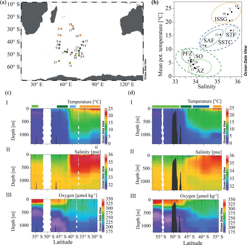
Figure 4. (a) Eukaryotic and (b) prokaryotic community structures of different water masses measured during the MD206 cruise. Redun-
dancy analysis (RDA) of 18S and 16S rRNA gene ASV tables as response variables and environmental metadata as explanatory variables;
environmental metadata are represented as arrows. Constrained analyses were performed by water mass. There were significant relation-
ships between water masses and community dissimilarities (PERMANOVA, 999 permutations; p < 0.001, R 2 = 0.67 for eukaryotes and
p < 0.001, R 2 = 0.74 for prokaryotes). Colors indicate major water masses according to the legend: yellow bar highlights the Indian South
Subtropical Gyre (ISSG), light blue bar highlights the Subtropical Front (STF), blue bar highlights the Subantarctic Front (SAF), dark green
bar highlights the Polar Front Zone (PFZ), and light green bar highlights the Antarctic Zone (AZ). Eukaryotic (c) and prokaryotic (d) general
dissimilarity model (GDM) with (I) observed compositional dissimilarity against predicted ecological distance, calculated from temperature
+ dissolved oxygen + NO− +
3 + NH4 + Si + chl a + PP + N2 fixation; (II) observed compositional dissimilarity against predicted composi-
tional dissimilarity to test the model fit; and contribution of (III) PP and (IV) N2 fixation to community dissimilarity expressed as a function
of the environmental parameter (f (PP) and f (N2 fix), respectively). For all functional plots of environmental data of the GDM analysis, see
Fig. S11. Eukaryotic (e) and prokaryotic (f) UpSet plots of ASV intersections between Longhurst provinces. Analyses are based on binary
tables (presence or absence) and the sum of all ASVs found across samples within one province. Intersection size shows number of ASVs
shared between provinces (black dots, associated) and ASVs only found in one province (only black dot). Set size shows number of ASVs
found in a specific Longhurst province.
9.51 % of the differences in community dissimilarity be- contributing 3.07 % to the community dissimilarity between
tween the SO and ISSG). Moreover, 4.79 % of the differ- the SSTC and the ISSG.
ences in community dissimilarity between the SO and the
SSTC were associated with a higher ASV count of Bacillar- 3.6 Prokaryotic community composition
iophyta_X ASVs in the SO. Further, we identified 10 ASVs
belonging to the phylum Dinophyceae, contributing 2.1 % to From each of the 14 stations, a fragment of the small sub-
the community dissimilarity structure between the SO and unit ribosomal RNA gene (16S rRNA) was amplified and
ISSG and 5.79 % to the community dissimilarity structure sequenced to obtain insights into the diversity and com-
between the SSTC and ISSG. This was further supported by munity composition of prokaryotes. A total of 1308 ASVs
relatively high concentrations of the photosynthetic pigments were recovered from which we removed 267 ASVs annotated
chl c3 and peridinin (both indicative pigments for dinoflagel- as chloroplasts and 68 ASVs annotated as mitochondria.
lates) in the SO and SAF. We found a relatively high number Prokaryotic richness increased with increasing sea surface
of ASV94 and ASV23 (Chloroparvula pacifica) in the SSTC, temperature (Pearson correlation: r = 0.65, p value = 0.03,
n = 11; Fig. S7a). Maximum alpha diversity (inverse Simp-
https://doi.org/10.5194/bg-18-3733-2021 Biogeosciences, 18, 3733–3749, 20213742 C. Hörstmann et al.: Microbial provincialism in the southern Indian Ocean
son) estimate was found in the SAF (81.92, station 15; and Planktomarina (Alphaproteobacteria) (5.69 % of the to-
Fig. S7d). Prokaryotic alpha diversity (inverse Simpson) was tal difference in community dissimilarity, SIMPER analysis,
positively (but not significantly) linked to primary produc- Table S6). Further, the SO had distinct ASVs belonging to
tivity (r = 0.36, p = 0.55, n = 11; Fig. S7f) but showed a the SUP-05 cluster, contributing 2.56 % (ASV_12) to the dif-
significant negative correlation with N2 fixation (r = −0.7, ference between SO and SSTC. The ISSG was characterized
p = 0.05, n = 11; Fig. S7h). by a high number of Cyanobacteria and some Actinobacteria.
Our RDA of the prokaryotic ASV table captured 90 % of The cyanobacterial fraction was dominated by Prochlorococ-
the total variance with a p value of 0.06 (permutations = 999, cus and Synechococcus.
n = 11). Sites clustered into Longhurst provinces along Within the class level, all stations were dominated by
the first two RDA axes (62.48 % of variance constrained; Alpha- and Gammaproteobacteria, Bacteroidia, Oxyphoto-
Fig. 4b). This was also shown in the PERMANOVA solution bacteria (Cyanobacteria), and Verrucomicrobia. Within the
for Longhurst provinces (permutations = 999, R 2 = 0.62, Alphaproteobacteria, we found a great dominance of eco-
p < 0.001, n = 11) and our PERMANOVA grouping into types I, II, and IV of SAR11 clade throughout all sam-
water masses (permutations = 999, R 2 = 0.74, p < 0.001, ples (Table S4). The relative number of pseudocounts of
n = 11; Fig. 4b). We found more ASVs occurring in either bacteria belonging to the phylum Bacteroidetes decreased
the ISSG or the SO provinces rather than across all provinces towards warmer SST in the ISSG, with significant differ-
(Fig. 4f). Further, the ISSG and the SO shared the least ASVs ences between the SO and ISSG (Welch two-sample t test
(Fig. 4f). In the RDA, sites within the ISSG province were t = 4.58, p < 0.001, n1 = 341, n2 = 151). The phylum Bac-
positively associated with SST and N2 fixation. Sites belong- teroidetes was largely dominated by the order Flavobacte-
ing to the SO were positively associated with dissolved in- riales (90.98 % of annotated ASVs). Cyanobacteria mainly
3−
organic nutrients (NO− 3 , PO4 , Si), dissolved oxygen, and occurred in the SSTC and in the ISSG, which were domi-
chl a concentrations as well as high PP (Fig. 4b). The com- nated by Prochlorococcus in the ISSG and Synechococcus in
munity composition within the SSTC (STF and SAF) was the SSTC. Cyanobacterial pseudocounts were significantly
distinct from that of the ISSG and SO along the second RDA lower in the SO in comparison to the SSTC (Welch two-
axis (21.67 % variance constrained) and positively associ- sample t test, t = −3.86, p value < 0.001, n1 = 17, n2 = 31)
ated with NH+ 4 concentrations (Fig. 4b). Linear relationships and to the ISSG (Welch two-sample t test, t = −4.74, p <
between beta diversity and rates were weak for PP (PER- 0.001, n1 = 17, n2 = 45). Atelocyanobacteria (UCYN-A)
MANOVA; permutations = 999, R 2 = 0.31, p = 0.007, n = ASVs occurred in the SAF (station 14) and ISSG (stations 2,
11) and N2 fixation (PERMANOVA; permutations = 999, 3).
R 2 = 0.2, p = 0.05, n = 11).
Investigating whether and at which magnitude envi-
ronmental parameters have an effect on prokaryotic mi- 4 Discussion
crobial community dissimilarity, our general dissimilarity
model (GDM) showed the expected curvilinear relationship Each water mass in our study had a distinct microbial fin-
(Fig. 4d I). Based on I-spline magnitude, geographic dis- gerprint, including unique communities in frontal regions.
tance had little effect on community dissimilarity. The largest We highlight clear relationships between microbial diver-
magnitude in community dissimilarity could be observed be- sity, primary productivity, and N2 fixation (high linear and
tween 190–1200 µmol C L−1 d−1 (Fig. 4d III). Community nonlinear covariability) in the southern Indian Ocean Gyre
dissimilarity changed most notably in response to variabil- (ISSG), the Southern Ocean (SO), and their frontal transi-
ity in low magnitudes of N2 fixation and did not change tion zone. Below, we discuss how this clear provincialism of
in samples with highest average N2 fixation measurements microbial diversity is disconnected from regional gradients
(2.8 nmol N L−1 d−1 station 3, and 4.0 nmol N L−1 d−1 sta- in primary productivity (PP) and N2 fixation across our tran-
tion 18). Largest magnitudes of community dissimilar- sect. This could suggest that microbial phylogenetic diversity
ity were associated with dissolved oxygen concentrations is more strongly bounded by physical oceanographic bound-
(Fig. S11b). aries, while microbial activity (and thus, perhaps, their func-
Taxonomically, based on analysis of the CLR-transformed tional diversity, not assessed here) responds more to chemical
ASV table, the prokaryotic community was dominated by properties that changed more gradually between the low- and
Proteobacteria, Cyanobacteria, and Bacteroidetes, which are high-nutrient provinces we sampled.
all typical clades for surface water samples (e.g., Biers et
al., 2009). The greatest community differences occurred be- 4.1 N2 fixation and associated microbial diversity
tween stations of the Southern Ocean (SO) and the Indian display distinct regional variations
South Subtropical Gyre (ISSG) provinces. Structure in com-
munity dissimilarity between the ISSG and SO were mostly Overall, our N2 fixation (up to 4.4 ± 2.5 nmol N L−1 d−1 )
associated with the number of Flavobacteriaceae (11.52 % of was comparable to N2 fixation measured by González
total community dissimilarity, SIMPER analysis, Table S6) et al. (2014) above the Kerguelen Plateau (up to
Biogeosciences, 18, 3733–3749, 2021 https://doi.org/10.5194/bg-18-3733-2021C. Hörstmann et al.: Microbial provincialism in the southern Indian Ocean 3743 10.27 ± 7.5 nmol N L−1 d−1 ) and showed a similar latitudi- coast of Chile and Peru with rates up to 190 µmol N m−2 d−2 nal trend as N2 fixation further east in the Indian Ocean, (Fernandez et al., 2011); and across the eastern Indian Ocean although with around 10-fold lower absolute rates (0.8–7 (Raes et al., 2015). This evidence counters the hypothesis of vs. 34–113 nmol N L−1 d−1 ; Raes et al., 2014). We note that Breitbarth et al. (2007) that N2 fixation occurs only when the localized rates reported by González et al. (2014) are to other sources of N are limited. The contribution of N2 fixa- date the only published N2 fixation measurements in this re- tion to the N pool – and thus to productivity – varies strongly gion, likely to be close to the annual maxima because of with ecosystem structure: in the SO, despite the local N2 - high irradiance; however, further investigations across sea- fixation measurements, N2 fixation remains likely a very mi- sonal changes within the study area are needed to confirm nor contributor to the N required by the microbial community our observations. Our regional data are therefore important in for primary productivity. closing the gaps in N2 fixation measurements in the Southern Our results also strongly suggest that prokaryotic commu- Ocean, especially considering that large disagreements exist nity structure and composition (beta diversity) were strongly between models of high-latitude N2 fixation rates (Tang et impacted by the presence of biological N2 fixation, which al., 2019). is itself a prokaryotic process (Karl et al., 2002). For exam- N2 fixation measurements often show high basin-wide ple, the N2 -fixing Atelocyanobacteria (UCYN-A) occurred variability as well as high variability between samples at in the SAF and ISSG; however, to gain a clear insight into the same site, being sensitive to details of experimental de- the community and N2 fixation, the diazotrophic community sign, incubation, and sea-state conditions (Mohr et al., 2010). would need to be further resolved by amplicon analysis of In aggregate, these issues are best accounted for by cal- functional (nifH) genes (Luo et al., 2012) as shown in other culating the minimum quantifiable rate (MQR; Gradoville high-latitude studies (Fernández-Méndez et al., 2016; Raes et al., 2017). We observed high heterogeneity of biologi- et al., 2020). cal samples taken from the underway flow-through system 5 min apart (separated by ∼ 15 km) within the same water 4.2 Total and specific primary productivity mass. Similar variability in absolute measurements of N2 fix- differentially affect microbial diversity ation (2.6–10.3 nmol N L−1 d−1 ± 7.5 nmol N L−1 d−1 ) were reported by González et al. (2014) close to our sampling site We found PP was highest in the PFZ and decreased towards around Kerguelen island. This could imply a sub-mesoscale higher latitudes in the SO (Fig. 3a). Strass et al. (2002) variability or influence of other unmeasured parameters. showed that frontal maxima of PP are expected, and the ob- As oligotrophic gyres extend and displace southwards un- served decrease was probably due to Fe limitation in the SO der climate change (Yang et al., 2020), the biogeochem- (Blain et al., 2008). Primary productivity can also be limited ical and physical characteristics of the SO are changing by Si concentration and light availability when the mixed (Caldeira and Wickett, 2005; Swart et al., 2018), and bi- layer deepens (Boyd et al., 2000), but in our data Si con- ological regional N2 fixation might become an important centrations were high in the surface water samples, and light N source for productivity. Our data showed maximal N2 fix- levels were close to maximum in austral summer. The mea- ation in the oligotrophic waters of the ISSG; however, no- sured maximum PP above the Kerguelen Plateau (station E) tably, measurable N2 fixation occurred well into the SO, was likely stimulated by Fe inputs (Blain et al., 2007). to 56◦ S, suggesting that N2 fixation contributes to the re- Our results did not support prior observations that frontal gional N pool, despite other available sources of N (Sh- regions (SAF and STF) supported higher specific primary iozaki et al., 2018; Sipler et al., 2017). Similarly, we found productivity (P B ) (as reported in the Antarctic Atlantic sec- a negative N∗ in the SO, which potentially indicates a P tor; Laubscher et al., 1993). While phytoplankton community excess supporting N2 fixation (Knapp, 2012). Noteworthy composition, phytoplankton size distribution, and nutrient is a slight increase in N2 fixation in the Antarctic Zone concentrations were strikingly different between the ISSG (AZ). High-latitude measurements in northern polar regions and SO, we found little difference in P B , with some slightly (Bering Sea) reached 10–11 nmol N L−1 d−1 (Shiozaki et al., lower values observed within the SSTC (Fig. 3b). Differ- 2017), substantially higher than our measurements of the SO ences in P B usually arise from physiological changes due (0.8–1.9 nmol N L−1 d−1 ), potentially supported by the close to variabilities in irradiance (Geider, 1987), nutrient concen- proximity to the coast or other factors such as day length, trations (Behrenfeld et al., 2008; Chalup and Laws, 1990), seasonality, diazotroph community, or trace metal concentra- or differences in phytoplankton community structure, where tions. cyanobacteria have the highest PP efficiency and diatoms the Our results suggest that regional N2 fixation was not lim- lowest (Talaber et al., 2018). Thus, our observations suggest ited by the presence of other sources of bioavailable N that either (1) there is a lack of selective pressure on pho- (Fig. S10); this is a conclusion also reached in a number of tosynthetic efficiency between provinces or (2) mechanisms studies including culture experiments (Boatman et al., 2018; driving P B are different between provinces, and the sum Eichner et al., 2014; Knapp, 2012), as well as in situ mea- of beneficial (e.g., increased nutrient concentrations in the surements in the South Pacific (Halm et al., 2012); off the SO) and detrimental mechanisms (e.g., low irradiance and https://doi.org/10.5194/bg-18-3733-2021 Biogeosciences, 18, 3733–3749, 2021
3744                                            C. Hörstmann et al.: Microbial provincialism in the southern Indian Ocean

photoinhibition through deep vertical mixing, reported from        rina belonging to the Roseobacter clade affiliated (RCA) sub-
the Antarctic circumpolar current (ACC); Alderkamp et al.,         group had relatively high proportions in the SO and is gener-
2011) result in similar P B . The slight variation around the      ally suggested to occur in colder environments (Giebel et al.,
frontal system is hard to interpret, as the complex interplay      2009) and previously detected in the Polar Front (Wilkins et
between factors may result in stochasticity.                       al., 2013b). The RCA subgroup is known for dimethylsulfo-
   Primary productivity can be an important driver for (phy-       niopropionate (DMSP) degradation in phytoplankton blooms
logenetic) microbial alpha diversity (Vallina et al., 2014), es-   (Han et al., 2020). In addition to bacteria known to be as-
pecially within ocean provinces (Raes et al., 2018). While         sociated with phytoplankton, we also observed those which
our observational study only has a small number of samples         symbiose with other organisms (e.g., Georgieva et al., 2020),
within and between oceanic provinces (n = 12, nISSG = 4,           such as the sulfur oxidizing Thioglobaceae (SUP-05 clus-
nSSTC = 3, nSO = 4), it did suggest that further validation        ter), previously found in symbiosis with Myctophidae fish
of this assumption is needed. We observed that PP changed          near Kerguelen Islands (Gallet et al., 2019). While beyond
gradually across the sampling region and that local variabil-      the scope of this study, we encourage further investigations
ity in PP was high between samples taken ∼ 15 km apart             of such trans-kingdom functional interactions as they them-
within the SSTC and SO (Fig. 3a). These local variabilities        selves may offer regional insights.
can arise from complex physico-chemical interactions be-
tween the STF, SAF, and SO (Mongin et al., 2008). Counter          4.3   Implications for microbial regionality
to Vallina et al. (2014) and Raes et al. (2018), we found a
significant negative correlation between eukaryotic alpha di-      Microbial diversity was regionally constrained independent
versity and PP within the ISSG. Further, we found no corre-        of geographical distance (GDM analysis), but it was parti-
lation between eukaryotic diversity and PP within the SSTC         tioned into ocean provinces as repeatedly described for other
and SO and none between prokaryotic alpha diversity across         ocean basins such as the Pacific (Raes et al., 2018) and
all provinces (Fig. S7).                                           the Atlantic Ocean (Milici et al., 2016). This supports the
   In terms of beta diversity, we observed a structuring ef-       classical concept of microbial biogeography (Martiny et al.,
fect of PP for pigment, 16S rRNA gene, and 18S rRNA                2006). Further, we found that microbial beta diversity was
gene-derived diversity profiles (Figs. 4a, b, S5). Pigment         even better resolved by individual water masses, highlighting
analysis revealed that photosynthetic prokaryotic diversity is     the importance of including oceanographic boundaries that
strongly impacted by the relative abundance of Prochloro-          limit cross-front dispersal (Hanson et al., 2012; Hernando-
coccus, which does not generally occur in cold high-latitude       Morales et al., 2017; Wilkins et al., 2013a).
waters (> 40◦ S/N; Fig. S5) (Partensky et al., 1999) and, if          Our beta diversity analysis confirmed the findings by Bal-
so, only in low abundance (reviewed in Wilkins et al., 2013).      tar and Arístegui (2017), who found unique environmental
Our 16S rRNA gene analyses confirm these observations              sorting and/or selection of microbial populations in the SAF
showing that (1) picoplankton – and specifically Prochloro-        and STF. Further, we were able to link these communities
coccus – had relatively high proportions in the ISSG but           to high NH4 concentrations. This suggests high recycling of
very low in the SSTC, (2) Synechococcus dominated the              nitrogen sources within the microbial loop and potentially fa-
Cyanobacterial fraction in the SSTC, and (3) both Prochloro-       voring nitrification in this area (Sambrotto and Mace, 2000).
coccus and Synechococcus were not detected in the SO (Ta-          We also found increased dinoflagellate concentrations (PFT)
bles S4, S6). In the SSTC and SO, phytoplankton commu-             which have been described to grow well under NH4 con-
nities had high proportions of dinoflagellates (Dinophyceae)       ditions (Townsend and Pettigrew, 1997). Despite our small
and diatoms (Bacillariophyta) (up to 74 % of diatom diag-          sample size within the SAF and STF, we were able to de-
nostic pigment concentrations), which are known as essential       tect these characteristics, supporting the call from Baltar et
contributors to marine PP and microbial diversity (Malviya         al. (2016) for better integrating frontal zones in our under-
et al., 2016) and known to dominate the phytoplankton frac-        standing of microbial biogeography.
tion within the Polar Frontal Zone (PFZ), especially as the           Different trade-offs such as nutrient limitation and graz-
blooming season progresses (Brown and Landry, 2001).               ing can shape the microbial seascape (Acevedo-Trejos et al.,
   Further, our results show that phytoplankton community          2018). In our study, the deviation between PN : chl a was
structure appears to be tightly coupled to the occurrence of       large between the SO and IO with high PN : chl a ratios in the
specific heterotrophic organisms (Table S6) and thus may           ISSG (Fig. S4), which has been used as an indicator of a rela-
mediate an indirect effect of PP through microbial food webs       tively high abundance of heterotrophic microbes and protists
(as also noted in, e.g., Sarmento and Gasol, 2012). For ex-        over autotrophic organisms (Crawford et al., 2015; Hager et
ample, in areas of relatively high diatom concentrations, we       al., 1984; Waite et al., 2007). This would suggest that grazers
found increased proportions of Flavobacteria. These bacte-         formed a higher fraction of total biomass in the ISSG than in
ria specialize on successive decomposition of algal-derived        the SO. However, we did not measure zooplankton biomass
organic matter (Teeling et al., 2012) and are known asso-          or grazing rates, so this remains speculative.
ciates of diatoms (Pinhassi et al., 2004). Further, Planktoma-

Biogeosciences, 18, 3733–3749, 2021                                                  https://doi.org/10.5194/bg-18-3733-2021
You can also read