The potential of increasing man-made air pollution to reduce rainfall over southern West Africa - ACP
←
→
Page content transcription
If your browser does not render page correctly, please read the page content below
Atmos. Chem. Phys., 21, 35–55, 2021
https://doi.org/10.5194/acp-21-35-2021
© Author(s) 2021. This work is distributed under
the Creative Commons Attribution 4.0 License.

The potential of increasing man-made air pollution to reduce
rainfall over southern West Africa
Gregor Pante1,a , Peter Knippertz1 , Andreas H. Fink1 , and Anke Kniffka1,b
1 Instituteof Meteorology and Climate Research, Department Troposphere Research (IMK-TRO),
Karlsruhe Institute of Technology (KIT), Wolfgang-Gaede-Str. 1, 76131 Karlsruhe, Germany
a now at: German Meteorological Service, Frankfurter Str. 135, 63067 Offenbach am Main, Germany
b now at: German Meteorological Service – Research Centre Human Biometeorology,

Stefan-Meier-Str. 4, 79104 Freiburg, Germany

Correspondence: Gregor Pante (gregor.pante@dwd.de)

Received: 13 May 2020 – Discussion started: 29 May 2020
Revised: 25 September 2020 – Accepted: 10 November 2020 – Published: 4 January 2021

Abstract. Southern West Africa has one of the fastest-             is further enhanced by an increase in low-level cloudiness.
growing populations worldwide. This has led to a higher wa-        The large spatial extent of potentially aerosol-related trends
ter demand and lower air quality. Over the last 3 decades,         during the LDS is consistent with the stronger monsoon flow
most of the region has experienced decreasing rainfall dur-        and less wet deposition during this season. Negligible aerosol
ing the little dry season (LDS; mid-July to end of August)         impacts during the FRS are likely due to the high degree of
and more recently also during the second rainy season (SRS;        convective organization, which makes rainfall less sensitive
September–October), while trends during the first rainy sea-       to surface radiation. The overall coherent picture and the ac-
son (FRS; mid-May to mid-July) are insignificant. Here we          celerating trends – some of which are concealed by SST ef-
analyse spatio-temporal variations in precipitation, aerosol,      fects – should alarm policymakers in West Africa to prevent
radiation, cloud, and visibility observations from surface sta-    a further increase in air pollution as this could endanger wa-
tions and from space to find indications for a potential contri-   ter supply and food and energy production for a large and
bution of anthropogenic air pollution to these rainfall trends.    growing population.
The proposed mechanism is that the dimming of incoming
solar radiation by aerosol extinction contributes to reducing
vertical instability and thus convective precipitation. To sep-
arate a potential aerosol influence from large-scale climatic      1   Introduction
drivers, a multilinear-regression model based on sea-surface
temperature (SST) indices is used. During both LDS and             Sub-Saharan Africa in general, but particularly the already
SRS, weakly statistically significant but accelerating nega-       densely populated southern West Africa (SWA hereafter),
tive rainfall trends unrelated to known climatic factors are       currently experiences strong population growth and urban-
found. These are accompanied by a strong increase in pol-          ization (United Nations, 2019). Together with economic
lution over the upstream tropical Atlantic caused by fire          growth in many sectors, this leads to an increasing demand
aerosol from Central Africa, particularly during the LDS.          for water. Currently, agricultural food production in SWA
Over southern West Africa, no long-term aerosol records are        is mostly rain-fed, with only basic or no irrigation systems
available, inhibiting a direct quantification of the local man-    in place (e.g. Namara and Sally, 2014). In addition, hydro-
made effect. However, significant decreases in horizontal vis-     power is a crucial contribution to electricity production in
ibility and incoming surface solar radiation are strong indi-      many countries across SWA (e.g. Lake Volta in Ghana, cf.
cators for an increasing aerosol burden, in line with the hy-      Henley, 2019), which further increases demand. Together
pothesized pollution impact on rainfall. The radiation trend       this creates a vulnerability to climate variability and long-
                                                                   term change, in particular with respect to rainfall (World

Published by Copernicus Publications on behalf of the European Geosciences Union.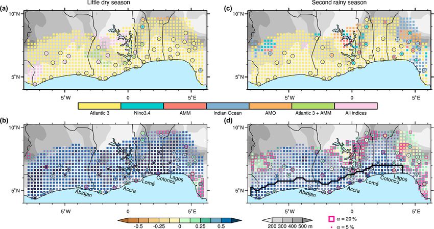
36                                                                  G. Pante et al.: Impacts of air pollution on rainfall over SWA

Bank, 2012). Understanding the causes of rainfall variability           this period (Giglio et al., 2006; Zuidema et al., 2016; Das et
and trends, particularly on interannual to decadal timescales,          al., 2017). Comparing precipitation over SWA on clean and
is crucial to make reliable predictions that allow the develop-         polluted days suggests a suppressing effect of the aerosol, but
ment of strategies for mitigation and adaptation.                       it is difficult to establish a causal relationship due to strong
   The climate of SWA is strongly controlled by the seasonal            covariance with meteorological variables, in particular low-
evolution of the West African monsoon. The main dry sea-                level wind that changes from southerly on polluted days to
son, when the convective zone lies further south, only lasts            easterly on clean days. One should therefore be cautious to
from December to February. The long wet period peaks dur-               link long-term aerosol changes with trends in precipitation
ing mid-May to mid-July (first rainy season; FRS) and in                based on these results. Unfortunately, there are no aerosol
September–October (second rainy season; SRS), interrupted               observations of sufficient quality over a long-enough time
by the so-called little dry season (LDS) (e.g. Thorncroft et al.,       period over SWA itself as satellite data suffer greatly from
2011; Fink et al., 2017; Maranan et al., 2018). Meteorologi-            frequent cloud contamination (Hsu et al., 2012). This hin-
cal conditions vary markedly between these four seasons and             ders establishing a more direct point-to-point relationship of
need to be taken into account to understand trends and vari-            aerosol with precipitation.
ability. On interannual to decadal timescales, SWA is sub-                 The recent Dynamics–Aerosol–Chemistry–Cloud Interac-
ject to marked rainfall variability, which has been linked to           tions in West Africa (DACCIWA) project (Knippertz et al.,
fluctuations in sea-surface temperatures (SSTs) in the nearby           2015a) conducted extensive field measurements in June–
Atlantic Ocean, with a moderate influence from the Pacific              July 2016 (Flamant et al., 2018) accompanied by modelling
and Indian oceans (Sutton and Hodson, 2005; Rowell, 2013;               experiments to better understand the role of aerosols in
Diatta and Fink, 2014). The 1980s stand out as a particularly           the West African monsoon system. DACCIWA studies con-
dry period, but both satellite- and station-based rainfall esti-        firmed the importance of an import of aerosol from fires in
mates show that SWA has undergone a mild recovery of rain-              Central Africa in addition to local pollution sources (Menut
fall since then, however with a large year-to-year variability          et al., 2018; Haslett et al., 2019a). The strong monsoon flow
(Sanogo et al., 2015). The contributions from the different             during the LDS causes a fast spread of pollutants from the
seasons to this trend vary, with rainfall increases during the          main sources in coastal cities inland (Deroubaix et al., 2019).
two rainy seasons (FRS and SRS) and a drying trend during               Given the overall high concentration of aerosol particles and
the LDS (Sanogo et al., 2015; Nicholson et al., 2018a, b).              predominantly stratiform clouds, relatively little susceptibil-
While SST changes appear to have played a role in creating              ity of cloud microphysics to aerosol effects was found (Deetz
this trend (Diatta and Fink, 2014), the magnitude of seasonal           et al., 2018b; Taylor et al., 2019). In contrast, the radiative
changes, i.e. the trends during the FRS, LDS, and SRS, re-              effect appears to be significant, particularly as the very high
mains poorly understood.                                                relative humidity in the moist, deep monsoon layer leads to
   There has been recent speculation about a local influence            wet growth of aerosol particles (Deetz et al., 2018a; Haslett et
of aerosol on rainfall in SWA (Knippertz et al., 2015b), an             al., 2019b). Combined with the high sensitivity of rainfall to
effect that has already been shown for southern Africa (Hod-            destabilization by local radiative heating found by Kniffka et
nebrog et al., 2016) and eastern China (Huang et al., 2016)             al. (2019), this creates potential for a significant direct effect.
for example. The basis for this is the dramatic increase in             Consistently, sensitivity experiments have shown that chang-
anthropogenic air pollution over recent decades (Liousse et             ing anthropogenic emissions along the Guinea coast has the
al., 2014), the predominant source of aerosol in the region             potential to shift the entire monsoonal rainband (Menut et
(Bauer et al., 2019). Aerosol particles can modulate rainfall           al., 2019) and regional circulation. However, climate models
through radiative (direct) and cloud (indirect) effects (Hay-           show substantial uncertainties in simulating the West African
wood and Boucher, 2000). Absorption and scattering reduce               monsoon system (Roehrig et al., 2013; Hannak et al., 2017),
the amount of solar radiation penetrating to the surface (dim-          casting doubt that realistic aerosol effects can be quantified
ming), thereby increasing vertical stability and suppressing            with confidence using modelling approaches.
convective rainfall. Some aerosols act as cloud condensa-                  The goal of this paper is to provide new evidence that
tion or ice nuclei, thereby influencing cloud microphysics,             the documented strong increases in anthropogenic emissions
albedo, and lifetime. The impact of this on precipitation is            in SWA and biomass-burning aerosol imports from Cen-
complex and depends on the cloud type and meteorological                tral Africa have significantly affected decadal rainfall trends.
setting.                                                                Based on the recent DACCIWA results, we hypothesize that
   Ajoku et al. (2020) recently produced daily composites for           aerosol has a suppressing effect due to dimming, in partic-
August 2003–2015 based on aerosol optical depth (AOD)                   ular during the LDS, when rainfall is mostly locally trig-
estimates from the Modern-Era Retrospective analysis for                gered (Maranan et al., 2018). For the FRS and SRS we ex-
Research and Applications, Version 2 (MERRA-2) over the                 pect a lesser import of aerosol from Central Africa (Giglio
Guinea coastal zone (5–10◦ N, 10◦ W–10◦ E), which is af-                et al., 2006), less spreading of coastal pollution inland due
fected by the advection of burning aerosol from mostly man-             to weaker monsoon winds, and more wet deposition due
made agricultural and forest fires in Central Africa during             to the enhanced rainfall (see also the discussion of Fig. 3

Atmos. Chem. Phys., 21, 35–55, 2021                                                          https://doi.org/10.5194/acp-21-35-2021
G. Pante et al.: Impacts of air pollution on rainfall over SWA                                                                 37

in Sect. 3.1). Given the lack of adequate aerosol observa-        5 d (pentad). First, the pentad estimates based on thermal
tions and issues with numerical models as described above,        infrared are corrected through local regression between
we chose to concentrate solely on long-term observations of       cold-cloud-top duration and Tropical Rainfall Measuring
rainfall, radiation, and visibility from surface stations com-    Mission (TRMM) 3B42 precipitation (Huffman et al., 2007).
bined with selected satellite products. Seasonality, spatial      In the second step, the product of the infrared estimates and
distribution, and qualitative meteorological arguments are        CHPClim is bias-corrected using 5 d accumulated gauge
used in the evaluation and interpretation of observed trends,     observations. The disaggregation to daily values is done us-
while influences of other climatic factors such as SST varia-     ing infrared-based cold-cloud duration. Despite the product
tions are eliminated on the basis of a multilinear-regression     being relatively insensitive against changes in the station
model. In Sect. 2 we describe rainfall and other data sets used   network (Chris Funk, personal communication, 6 July 2018)
in this study together with a description of the techniques       and a successful use in trend studies in SWA (e.g. Bichet
employed for the trend analysis. Section 3 contains a short       and Diedhiou, 2018), large changes in surface station avail-
discussion of the climatological background of our study re-      ability (e.g. https://data.chc.ucsb.edu/products/CHIRPS-2.0/
gion followed by a detailed analysis of rainfall and aerosol      diagnostics/stations-perMonth-byCountry/pngs/Benin.003.
trends. We summarize the main results and draw conclusions        station.count.CHIRPS-v2.0.png, last access: 8 May 2020)
in Sect. 4. Results for the FRS, which is not in the focus of     may induce inhomogeneities in long-term trends. This has
this paper, are provided for completeness in the Supplement.      been noticed by Diem et al. (2019) for western Uganda,
                                                                  who stress the necessity to validate satellite-derived trends
                                                                  by ground-based measurements. Furthermore, the algorithm
2     Data and methods                                            tends to smooth spatial inhomogeneities.
                                                                     Therefore as an additional source of precipitation data in
2.1    Region and season definition
                                                                  the region, the Karlsruhe African Surface Station Database
For the definition of seasons, we follow the description al-      (KASS-D), containing daily, quality-controlled rain gauge
ready given in Sect. 1: FRS (15 May–14 July), LDS (15 July–       measurements from manned weather stations operated by na-
31 August), and SRS (1 September–31 October). Figure 1            tional weather services (e.g. Vogel et al., 2018), has been
shows a map of the region of interest in SWA. Longitudi-          used in this study. Only stations with at least 50 % data cov-
nally we concentrate on the region 8◦ W–6◦ E, which avoids        erage are considered to allow a meaningful trend analysis. As
higher topographic features and contains all major cities         this criterion is hardly fulfilled before 1983 and after 2015,
along the Guinea coast such as Abidjan, Accra, and Lagos          the main analysis is restricted to this period. In addition, the
as well as Kumasi in inland Ghana. Our main region of study       trend analysis is repeated for the more recent, shorter time
reaches 3.5◦ of latitude inland from the coastline (red border    span 2001–2017, for which surface observations of incom-
in Fig. 1), a distance for which we suppose to find aerosol       ing solar radiation and more satellite data are available (see
effects on precipitation due to the fast northward transport      Sect. 2.4). Unfortunately, the availability of KASS-D data
of pollutants from the cities with the monsoon flow during        deteriorates during this period, mostly in Nigeria, where our
the LDS. As during the SRS the monsoon flow weakens con-          database has few data after 2015. Despite this, we decided
siderably, implying that pollutants will remain in the densely    not to end this recent period in 2015 because trends become
populated coastal plains, we concentrate on a smaller region,     less meaningful for shorter time spans. Note that in the 1990s
referred to as “coastal strip”, during this season (blue border   to 2010s, KASS-D contains daily data from many stations in
in Fig. 1). The coastal strip only reaches 0.75◦ inland and       SWA that have not been used in CHIRPS.
is restricted to 8◦ W–4◦ E due to the strong curvature of the
coastline to the east of Lagos.                                   2.3   Other surface, satellite-based, and reanalysis data
                                                                        sets
2.2    Rainfall data sets and investigation period
                                                                  Visibility and low- and medium-cloud-cover data from the
Two different rainfall data sets are used in this study: first,   Met Office Integrated Data Archive System (MIDAS) (Met
the Climate Hazards Group InfraRed Precipitation with             Office, 2006) are used from those stations in SWA where
Stations (CHIRPS, Funk et al., 2015a) data set. It utilizes       data are available for at least 50 % of the days in each sea-
both high-resolution satellite imagery and in situ station        son. Horizontal-visibility data are categorized into ranges of
data and provides, amongst other things, daily rainfall           “below 10 km”, “10–20 km”, and “above 20 km”, for which
estimates over land on a 0.25◦ × 0.25◦ horizontal grid            time series and trends are calculated. Observations of sur-
from 1981 onwards. CHIRPS uses an underlying static               face downwelling shortwave radiation (SDSR) are avail-
rainfall climatology (CHPclim; Funk et al., 2015b), which         able at Parakou (October 2001–June 2017) and Lamto (Jan-
contains input from historical station precipitation averages,    uary 2001–May 2018). The instrument in Parakou was re-
historical thermal infrared satellite estimation averages, and    placed in March 2009 and again in March 2014, potentially
a global topographic grid. The analyses are performed every       influencing trend calculations due to inconsistencies in the

https://doi.org/10.5194/acp-21-35-2021                                                  Atmos. Chem. Phys., 21, 35–55, 2021
38 G. Pante et al.: Impacts of air pollution on rainfall over SWA
Figure 1. Geographical overview. Map of southern West Africa showing major cities, topographic features, and the areas used for spatial
averaging in this paper. The red bordered region is analysed for the little dry season (LDS), while only the blue bordered region, referred to
as “coastal strip”, is considered for the second rainy season (SRS).
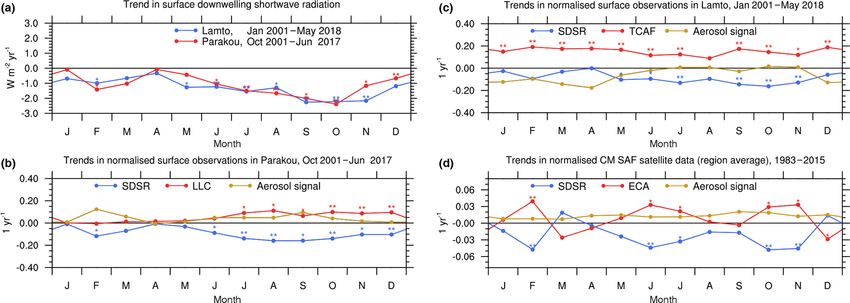
measurements. However, a shorter time series (2002–2015) To give climatological context to the trend analysis pre-
from Djougou, about 100 km north-east of Parakou, indicates sented here, relative humidity, cloud cover, and meridional
that the observations in Parakou are consistent (not shown). wind speed data from the fifth generation of European Cen-
No visibility data are available for Lamto, but human ob- tre for Medium-Range Weather Forecasts (ECMWF) at-
server estimates of total cloud area fraction (TCAF) are avail- mospheric reanalyses of the global climate (ERA5; Hers-
able for January 2000–July 2016. From these (sub-)daily ob- bach et al., 2020) are used. The influence of ocean tem-
servations seasonal and monthly averages were calculated, peratures on rainfall is analysed using the five most im-
again with a 50 % data coverage criterion. For a more com- portant SST-based climate indices for the region, namely
plete look at radiation, monthly data of SDSR and effective Atlantic 3 (3◦ S–3◦ N, 0–20◦ W), Niño3.4 (5◦ S–5◦ N, 120–
cloud albedo (ECA) of the SARAH-2 data set from the Satel- 170◦ W), the coupled ocean–atmosphere Atlantic Meridional
lite Application Facility on Climate Monitoring (CM SAF; Mode, Indian Ocean (10◦ S–30◦ N, 50–90◦ E), and the At-
Pfeifroth et al., 2017) are analysed. The comparison of nor- lantic Multidecadal Oscillation index (Atlantic Ocean from
malized trends (see Sect. 2.4) of SDSR and ECA allows us to 0–70◦ N), all as used by Diatta and Fink (2014). The At-
estimate a residual potentially related to aerosol. This tech- lantic Meridional Mode is based on the National Centers
nique of normalization is also applied to observations from for Atmospheric Prediction/National Center for Atmospheric
the surface stations in Parakou and Lamto. Research (NCEP/NCAR) reanalysis and the Atlantic Multi-
Monthly satellite measurements of aerosol optical depth decadal Oscillation index on the Kaplan SST data set. The
(AOD) on a 1◦ × 1◦ horizontal grid from the Moderate other three indices are computed from SST values from
Resolution Imaging Spectroradiometer (MODIS) (Plat- the Hadley Centre Sea Ice and Sea Surface Temperature
nick et al., 2017a), i.e. the “combined dark target and (HadISST) data set. The same weighting as for the AOD data
deep blue AOD at 0.55 µm for land and ocean: mean is used for the conversion from monthly climate indices to
of daily mean”, are used to calculate seasonal trends seasonal averages.
between July 2002 (beginning of data set) and Octo-
ber 2018. As these are monthly data, they are weighted 2.4 Methods for trend analysis
when calculating season-averaged values. AOD for the
LDS (15 July–31 August), for instance, is computed as Long-term trends for seasonal rainfall totals are computed
AOD(LDS) = (0.5 × AOD(July) +1.0 × AOD(August))/1.5. for every CHIRPS grid point and KASS-D station, applying
Especially over land, clouds often inhibit AOD measure- Sen’s slope method (Sen, 1968; Hirsch et al., 1982; Hipel
ments from space, leading to many missing values in the and McLeod, 1994). It calculates slopes for each pair of 2
MODIS monthly products. To cover the diurnal cycle, only consecutive years in a time series, and the final trend is the
months are used when AOD data from both the Aqua and median from all slopes. These trends are tested on statisti-
Terra platforms are available, which are then averaged to cal significance using the Mann–Kendall test (Mann, 1945;
obtain one single monthly value. For every year a seasonal Davison and Hinkley, 1997; Hipel and McLeod, 2005). Gen-
mean value is computed if data are available for all months erally, trends are considered statistically different from 0 if
of the respective season. Again a sufficiently complete the two-sided p value is smaller than the tested significance
record with data for at least 50 % of the seasons between level α. All our tests are performed for α values of 5 % and
2002 and 2018 is required before calculating a trend. 20 %, the latter being a relatively weak criterion for statis-
tical significance. As discussed in the context of “climate
Atmos. Chem. Phys., 21, 35–55, 2021 https://doi.org/10.5194/acp-21-35-2021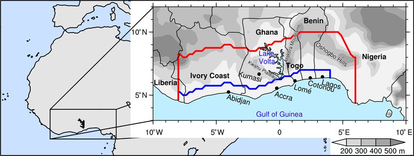
G. Pante et al.: Impacts of air pollution on rainfall over SWA                                                                   39

change attribution” by Lloyd and Oreskes (2018) and Knut-           Atlantic 3 index alone yields best results for a large majority
son et al. (2019), the choice of significance levels depends on     of CHIRPS grid points analysed (yellow in Fig. 2a). This is
how one intends to interpret the results. Small α values reveal     consistent with previous results for a slightly larger region
high confidence that a trend found in the data has some other       along the Guinea coast and a longer season from June to
reason than natural variability. However, a less strict signif-     September (Diatta and Fink, 2014). Exceptions are (a) the
icance level (α = 20 % in our case) can still be useful for a       Kwahu Plateau in south-western Ghana (combination of At-
study like ours that is dealing with the challenge of a rela-       lantic 3 with the coupled ocean–atmosphere Atlantic Merid-
tively short and incomplete data record subject to multiple         ional Mode; green), (b) central Ghana and the far south-west
influence factors and possibly non-linearities. In such a situ-     of Ivory Coast (combination of all five climate indices; pink),
ation, choosing a large α implies reducing so-called “type II       and (c) northern Benin and adjacent Nigeria (Atlantic Multi-
errors”, i.e. retaining the null hypothesis of no trend beyond      decadal Oscillation index; orange), but this region consists
natural variability, although such a trend actually exists but      of only five grid points. The agreement between CHIRPS
is hard to detect with the information at hand. Taking into         and the stations is largely good, with the exceptions of Kara
account additional factors such as geographical distribution        in Togo (Atlantic Multidecadal Oscillation index; orange),
and seasonal behaviour can help in the evaluation of a trend        Sokodé in Togo (Niño3.4 index; turquoise), and Warri in
with weak statistical significance. Ultimately, it is the bal-      Nigeria (Indian Ocean; blue). We are not aware of any con-
ance of all available evidence that does or does not suggest        vincing physical reasons for these deviations and therefore
that an identified trend has other-than-natural causes (Knut-       mostly consider them to be statistical fluctuations. This is
son et al., 2019), and this is the philosophy we are following      consistent with Fig. 2b showing correlations with the best
in this study. We feel that such an approach is particularly        models to be above 0.5 through most of the region, largely
justified in the given situation as a risk assessment for a po-     irrespective of model choice. Only the orange points from
tential local human influence on rainfall in SWA is urgently        Fig. 2a at the far north-eastern fringe of the study region show
needed.                                                             a lower correlation, indicating problems with data or stronger
   Interannual variations in precipitation in SWA are, de-          terrestrial forcings farther away from the ocean. The simple
pending on the exact region and season, influenced by (re-          picture that emerges from this analysis is that a considerable
mote) climate indices. In order to distinguish between these        part of the season-to-season variability is linearly controlled
climatic signals and other parameters such as (local) air pol-      by the SST over the nearby Atlantic Ocean, with warmer wa-
lution, we calculate so-called “residual” time series through       ters leading to more rainfall. This is related to a weaker tem-
subtraction of a linear-regression model based on five climate      perature and pressure gradient towards the Sahel, which leads
indices defined in the previous section from the original time      to stronger convergence and higher moisture content in SWA
series. For each time series, 31 different linear models are        (Losada et al., 2010).
constructed that consist of either single indices (i.e. five lin-      The picture during the SRS is also dominated by the At-
ear models) or any combination of the five indices (i.e. 10         lantic 3 index, but in the northern and especially eastern parts
combinations with two indices, 10 combinations with three           of the region, other climate indices yield better linear models
indices, 5 combinations with four indices, and the one lin-         (Fig. 2c). Given the weaker monsoon flow during this sea-
ear model with all five indices). For each model the leave-         son, this may indicate a less close link to the nearby Atlantic
one-out cross-validation procedure (Efron and Tibshirani,           Ocean and more room for teleconnections to influence rain-
1997, for example) is performed and evaluated calculating           fall. Correlation coefficients are generally lower than dur-
the residual sum of squares. Aiming to keep the model as            ing the LDS but still reach 0.5 across considerable parts of
simple as possible, the linear regression was constructed to        the region, particularly along the coastal strip (marked by
consist of as few indices as possible to avoid (near) multi-        a black line in Fig. 2d). It is striking that the regions that
collinearity. However, if a combination of two indices yields       do not show the simplest model based on the Atlantic 3 in-
a model for which the residual sum of squares is at least 3 %       dex also show the lowest correlations, which again points to-
lower than that of a single-index linear model, the two-index       wards data problems and/or more local influences such as
model is chosen. A third, fourth, or fifth index is again only      topographic forcing by the Oshogbo Hills in Nigeria.
added if the performance of such a linear model increases by           During the FRS, the Atlantic 3 index is also dominating,
more than 3 % compared to a model consisting of fewer in-           but regions where other indices yield better linear models are
dices. Thresholds between 1 % and 5 % were tested for the           larger than during the other two seasons (Fig. S1a). The cor-
performance improvement but all result in the same choice           relation of the best models with rainfall is low during the
for the linear model at the majority of CHIRPS grid points          FRS, rarely exceeding values of 0.5 (Fig. S1b) and showing
and stations.                                                       a rather weak effect of ocean temperatures on rainfall during
   The optimal linear model determined this way and its cor-        this season. As before, the agreement between station and
relation coefficient with the original rainfall time series are     CHIRPS data in both the optimum index combination and
shown in Fig. 2 for the LDS and SRS during the 1983–2015            the correlation is very good.
period. During the LDS a simple linear model built on the

https://doi.org/10.5194/acp-21-35-2021                                                    Atmos. Chem. Phys., 21, 35–55, 2021
40 G. Pante et al.: Impacts of air pollution on rainfall over SWA
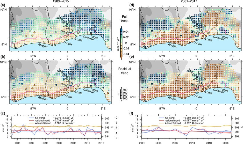
Figure 2. Optimal linear model. (a) Combination of climate indices yielding the best results with respect to the leave-one-out cross-validation
procedure as described in Sect. 2.2 for the LDS. Each of the single-index models (Atlantic 3, Niño3.4, AMM, AMO) can be found. The only
combinations of indices with better results are Atlantic 3 with AMM and the combination of all five indices. (b) Pearson’s correlation
coefficient of the optimal linear model with the original rainfall time series for the LDS. Panels (c) and (d) are the same as (a) and (b) but
for the SRS. The coastal strip is marked by a black line in (d). All panels show data from 1983–2015 for the CHIRPS (coloured pixels) and
station data (coloured circles). Statistically significant correlations in (b) and (d) are marked with pink borders of pixels and stations for the
α = 20 % level and a pink dot in the middle for the α = 5 % level, respectively.
The optimal linear models described above are now used (stationarity). If surface radiation was entirely determined by
to remove the dominant influences of SST fluctuations from cloud cover, identical but opposite normalized trends would
the original time series. Trends in these residual time series result. A non-zero sum of the normalized trends points to
will differ from those computed from the original time series, an additional aerosol effect and/or changes in cloud optical
and we refer to them as “residual” trends and “full” trends, thickness, which could at least in part be related to aerosol.
respectively. Trends and their statistical significance are also Positive sums (e.g. slight reduction in radiation but strong in-
calculated for all other observed parameters described in crease in cloud) would then indicate reduced aerosol, while
Sect. 2.3, namely visibility, clouds, radiation, and AOD, but negative sums (e.g. strong reduction in radiation but only
no residual time series are calculated in these cases. slight increase in cloud) point to increased aerosol. This con-
cept is applied to the time series of CM SAF satellite data and
2.5 Indirect indicators for aerosol trends surface observations from Parakou and Lamto in Sect. 3.3.
Another data set we use as an indirect aerosol indicator
Given the issues with aerosol observations in SWA described are surface observations of horizontal visibility as estimated
above, we have to rely on indirect indicators to determine by human observers. Trends in this parameter are most likely
changes in air pollution. These are observations of cloud an effect of changes in the aerosol burden, but changes in
cover, radiation, and horizontal visibility. As there is not low-level humidity and clouds may also have an effect as
sufficient information for even the simplest radiative trans- they change incoming light and the split between direct and
fer estimates, we chose to estimate a potential aerosol ef- diffuse radiation.
fect on radiation through considering normalized trends. In
this context, normalizing means subtracting the mean and di-
viding by the standard deviation of the respective time se- 3 Results
ries. The dimensionless trends in such normalized time series
can be directly compared to each other assuming no signif- In this section, trends in rainfall (Sect, 3.2) and various in-
icant changes in variance during the considered time period dicators of aerosol burden (Sect. 3.3.) are presented and re-
Atmos. Chem. Phys., 21, 35–55, 2021 https://doi.org/10.5194/acp-21-35-2021
G. Pante et al.: Impacts of air pollution on rainfall over SWA                                                                   41

lated to each other. To put the results into context, the short    centration to the vicinity of sources. Wet deposition will of
Sect. 3.1 summarizes the annual cycle of relevant meteoro-         course also be enhanced during the FRS.
logical variables.                                                    Another parameter of interest is the frequency of relative
                                                                   humidity of 95 % and higher (light-blue curves in Fig. 3) as
                                                                   this determines the potential for wet growth of aerosol parti-
3.1   Climatological conditions
                                                                   cles, which strongly enhances radiative effects (Deetz et al.,
                                                                   2018a; Haslett et al., 2019b). Here large differences are seen
Figure 3 shows the time mean seasonal evolution of key vari-       between the deep layer of very moist conditions in LDS as
ables based on ERA5 and CHIRPS rainfall averaged over the          compared to the much shallower layers in the rainy seasons,
main study region shown in Fig. 1. The main seasons as used        with maxima at 950 hPa (FRS) and even 975 hPa (SRS).
in this paper are delineated by vertical black lines. During the   Qualitatively, these results suggest that during the LDS the
main dry season from December to February, rainfall drops          potential for wet aerosol growth is higher and that consid-
to values well below 1 mm d−1 followed by a gradual ramp-          erable aerosol effects could in fact be spread over a much
up towards the FRS starting in mid-May. Peaks during the           larger region through the combination of faster transport and
two rainy seasons FRS and SRS reach about 8 mm d−1 , while         less wet removal than in the other seasons. For the LDS and
rainfall drops to below 4 mm d−1 during the LDS. The mon-          the SRS, time series of the frequency of relative humidity of
soonal retreat in October and November occurs much more            95 % and higher (Fig. 4) reveal slight decreases over 1983–
rapidly than the onset.                                            2015 of about 0.1 % yr−1 , which are significant only on the
   Maranan et al. (2018) recently developed a seasonal clima-      α = 20 % level. Given the highly non-linear dependence of
tology of rainfall types over the region based on satellite im-    wet growth of aerosol particles on relative humidity (e.g.
agery and reanalysis data. They found that the location of the     Haslett et al., 2019b), this relatively small change implies
African easterly jet close to the Guinea coast during the FRS      that the radiative effect per amount of dry aerosol will be
creates enhanced vertical wind shear, leading to the highest       smaller in the later part of the study period. As our estimates
degree of convective organization into long-lived mesoscale        for aerosol trends rely on horizontal visibility and surface ra-
clusters during the year (marked with ++ in Fig. 3). In con-       diation, the change in dry aerosol may be even larger than
trast, during the SRS, the vertical profiles of shear and insta-   deduced from these parameters alone. The trend of relative
bility lead to a more local convective triggering, for example     humidity exceeding 95 % during the FRS is indistinguishable
by the land–sea breeze, and therefore smaller and shorter-         from 0 (Fig. S2 top).
lived but often intense systems (+ in Fig. 3). Conditions dur-        Finally the red curve in Fig. 3 shows the mean vertical pro-
ing the LDS are significantly different. During this period,       file of cloud cover at 06:00 UTC (corresponds to local time
SWA is subject to a strong southerly monsoon flow, leading         in the study region), the analysis time closest to the diurnal
to fast advection of thermodynamic and chemical properties         maximum of low clouds (van der Linden et al., 2015). These
from the Gulf of Guinea, typically along a low-level jet that      clouds are crucial for the radiative energy budget and, thus,
forms at night. Rainfall during the LDS is often due to rela-      for vertical mixing and the triggering of convection in the
tively weak, isolated, short-lived, and weakly organized con-      afternoon (Kalthoff et al., 2018; Kniffka et al., 2019). We
vection (◦ in Fig. 3; Maranan et al., 2018), mostly occurring      anticipate this factor to influence the significance of aerosol
in the afternoon. Land–sea breeze days have a seasonal min-        changes to the surface energy balance when incoming radi-
imum (Guedje et al., 2019), and stability is often too high to     ation is strongly reduced by cloud cover. Peak coverage at
allow the transition from cumulus clouds in the coastal hin-       about 950 hPa differs only little between the three seasons,
terland into deep cold convective clouds in the course of the      but in the LDS the cloud layer is somewhat thicker.
afternoon.                                                            For the remainder of the paper, the analysis concentrates
   The arrows in Fig. 3 show average wind profiles for             on the LDS and the SRS, for which we found the largest indi-
the three seasons of interest. Clearly the monsoon flow is         cations for aerosol effects. The corresponding results for the
strongest in the LDS, reaching meridional wind speeds ex-          FRS are provided in the Supplement and are referred to along
ceeding 4.5 m s−1 at 950 hPa with southerly winds up to            the way. Figure 3 offers relatively little in terms of potential
875 hPa, marking the depth of the monsoon layer. The FRS is        reasons of fundamentally different behaviour in the FRS, so
also characterized by marked southerlies and an even deeper        we hypothesize that the much larger degree of convective or-
monsoon layer, while the SRS shows weaker flow reduced             ganization during this season found by Maranan et al. (2018)
to a shallower layer. This is consistent with Guedje et al.        is key in reducing sensitivity to local aerosol effects. In addi-
(2019), who investigated upper air data at the coastal station     tion, spatial patterns of positive and negative rainfall trends
of Cotonou. As already discussed earlier, we anticipate that       during FRS change depending on the time period analysed
this should restrict the largest aerosol effects to the coastal    (cf. Fig. S3a, b with S3d, e), and there are more pronounced
strip, which contains the main pollution sources. The higher       discrepancies between CHIRPS and station data. Regionally
rainfall in SRS as compared to the LDS should also lead to         averaged trends are weak and statistically not significant on
more wet deposition, which would further support the con-          the 20 % level (Fig. S3c, f).

https://doi.org/10.5194/acp-21-35-2021                                                    Atmos. Chem. Phys., 21, 35–55, 2021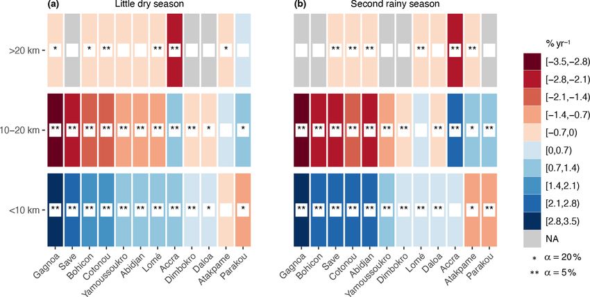
42                                                                      G. Pante et al.: Impacts of air pollution on rainfall over SWA

Figure 3. Climatological overview. Average annual cycle of meteorological conditions over southern West Africa (red bordered region in
Fig. 1). Solid black line shows mean rainfall (CHIRPS), while the profiles give average conditions (ERA5, mean 06:00 UTC values from
1983–2015) for meridional wind (southerly (northerly) wind as vectors to the right (left), strength according to the reference vector); cloud
cover (pink); and the frequency of relative humidity exceeding 95 % (cyan) for the first rainy season (FRS, 15 May–14 July), the little
dry season (LDS, 15 July–31 August), and the second rainy season (SRS, 1 September–31 October). Cloud cover and relative humidity
range from 0 to 1 according to the scales at the bottom for each season. Symbols below the seasons’ names mark the degree of convective
organization (++ strong, + moderate, ◦ weak) according to Maranan et al. (2018).

                                                                            der of Ivory Coast and Liberia. Large parts of Ivory Coast and
                                                                            Ghana show moderate drying, while trends over the eastern
                                                                            countries (Togo, Benin, Nigeria) are somewhat more mixed.
                                                                            Weakly positive trends are seen in the coastal plains between
                                                                            Accra and Lagos and in the far north, in the surroundings of
                                                                            the Atakora Mountains and the Oshogbo Hills. A remarkable
                                                                            pattern evident from Fig. 5a is that, while inland the agree-
                                                                            ment between stations and CHIRPS is largely good, many
                                                                            stations at the immediate coast show positive trends, some
                                                                            quite considerable ones, which are not always reflected well
                                                                            in CHIRPS. This points either to data problems in CHIRPS at
                                                                            the coast or to a very local effect, as for example related to the
Figure 4. Time series of relative humidity. Time series from 1983–
2015 and simple linear-regression lines show the temporal evolution         sea breeze (Guedje et al., 2019). There are indications that
of the frequency of relative humidity exceeding 95 % averaged from          the ongoing deforestation and urbanization along the coastal
925–975 hPa. Data are shown for the LDS (black) and the SRS (red)           strip enhance convective triggering during the afternoon due
and are spatially averaged over the entire study region (see Fig. 1).       to increased turbulent fluxes of sensible heat (Chris Taylor,
                                                                            personal communication, 28 April 2020).
                                                                               Despite the relatively high correlations with SSTs over the
3.2     Rainfall trends                                                     Atlantic (see Fig. 2), the residual trends (Fig. 5b) do not differ
                                                                            fundamentally from the full trends. The main reason for this
3.2.1    Little dry season                                                  is the small warming of the tropical Atlantic during this sea-
                                                                            son (Fig. 5c) that dominates the statistical model at the ma-
Figure 5 shows full (top row) and residual (i.e. with the in-               jority of grid points and stations (see Sect. 2.4). Amongst the
fluence of SST variations removed; see Sect. 2.4, middle                    few exceptions are central Ghana and western Ivory Coast,
row) rainfall trends for the LDS during 1983–2015 (left)                    which both show a combination of all five climate indices to
and 2001–2017 (right) for both surface station observations                 give the best statistical model (Fig. 2a). The Niño3.4 index,
and CHIRPS. The full trend over the long period 1983–2015                   for example, is anti-correlated with rainfall and increases
(Fig. 5a) largely confirms results by Sanogo et al. (2015)                  by 0.1 K per decade (not shown). This explains that resid-
of an overall drying in the region during the LDS. Largest                  ual trends are more positive than the full trends in regions
absolute decreases on the order of −0.04 mm d−1 yr−1 are                    where this index is part of the best linear model. Neverthe-
found over the wet Niger Delta region in the south-eastern                  less, overall the highly negative residual trend points to a pos-
corner of the study region and in the far west along the bor-               sible effect of increased dimming by aerosol. This would not

Atmos. Chem. Phys., 21, 35–55, 2021                                                              https://doi.org/10.5194/acp-21-35-2021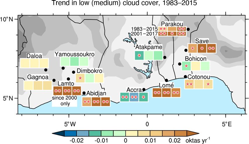
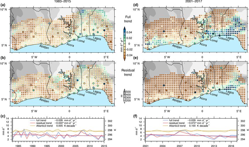
G. Pante et al.: Impacts of air pollution on rainfall over SWA                                                                                  43

Figure 5. Rainfall trends during the little dry season. (a–c) Trends in rainfall from 1983–2015 for CHIRPS data (coloured pixels) and station
data (coloured circles). Panels (d), (e), and (f) are the same as (a), (b), and (c) but for recent trends from 2001–2017. Shown are full (a, d) and
residual (b, e) trends. Note the overall good agreement between CHIRPS and station data. Topography is shown in grey shadings. “Residual”
in this context means that a statistical model was used to remove the influence of other known climatic factors on rainfall (for details, see
Sect. 2.4). Time series (c, f) of full (blue) and residual (red) CHIRPS rainfall, spatially averaged over the entire region, and the Atlantic 3
climate index (gold) are shown together with their trends over the respective time span. A * in (c) and (f) marks statistically significant trends
on the α = 20 % level.

stand in contrast with the positive trends at coastal stations as              The right-hand-side panels in Fig. 5 show the correspond-
also seen in Fig. 5b because the additional aerosol radiative               ing analysis for the shorter and more recent period 2001–
forcing needs time to take effect over land, while the imme-                2017. As for the longer period 1983–2015, there is a general
diate coast is dominated by advection from the ocean (and                   tendency for inland areas to dry, while coastal areas even get
was most strongly changed by urbanization). The positive                    wetter, but this contrast is now much sharper. Removing the
trends to the north of the Kwahu Plateau in central Ghana,                  contribution from an overall positive SST trend over the trop-
the Atakora Mountains in Togo and Benin, and the Oshogbo                    ical Atlantic of 0.1 K per decade (Fig. 5f) has a much larger
Hills in north-west Nigeria could be an indication of delayed               effect than for the longer period, with trends becoming more
convective triggering over higher ground due to the reduced                 negative practically everywhere. Positive values are now re-
solar insolation, allowing rainfall systems to travel further               stricted to the densely populated strip from Accra to Lagos,
downstream.                                                                 the latter by far the largest city of the region and subject to
   Figure 5c shows the CHIRPS trends averaged over all grid                 fast expansion. The area-averaged trend of the full time se-
points of the study region. Not surprisingly, both full and                 ries now amounts to −0.039 mm d−1 yr−1 , while the residual
residual time series are quite similar with relatively small                trend reaches −0.072 mm d−1 yr−1 , which is 2.4 times larger
trends as compared to the large interannual variability. Sub-               than for 1983–2015 and statistically significant on the 20 %
traction of the SST-based statistical model reduces the trend               level. This reduces typical monthly rainfall amounts from
from −0.026 to −0.022 mm d−1 yr−1 , but, since the interan-                 150 to 112 mm, i.e. by one-fourth, indicating that the effect
nual variability is also reduced, this leads to statistical signif-         we are postulating here is accelerating with the fast growing
icance on the 20 % level. The latter value translates to 23 mm              population.
per month over the 33-year period, which corresponds to
nearly 20 % of monthly rainfall during the LDS.

https://doi.org/10.5194/acp-21-35-2021                                                               Atmos. Chem. Phys., 21, 35–55, 2021
44                                                                G. Pante et al.: Impacts of air pollution on rainfall over SWA

3.2.2   Second rainy season                                           become restricted to central Ivory Coast, the northern Lake
                                                                      Volta, and smaller regions in Nigeria, while large parts of
The corresponding analysis for the SRS is shown in Fig. 6.            SWA show negative trends as low as −0.04 mm d−1 yr−1
The full long-term trend (Fig. 6a) is characterized by dry-           (Fig. 6e). The change is most dramatic east of Lake Volta
ing in southern Ivory Coast and southern Ghana, moderate              in Togo and Benin. Most of the large coastal cities, with the
moistening in central Ivory Coast and central Ghana, and              exception of eastern Ghana, now also show clearly negative
strongly positive trends in the north-east. Averaged over our         residual trends.
study region, the trend is positive, which is consistent with            Spatial averages over the coastal strip (Fig. 6f) show a cor-
recent studies by Bichet and Diedhiou (2018) and Nkrumah              responding shift to more negative trends. For the full time se-
et al. (2019). As for the LDS, the overall agreement be-              ries this amounts to −0.050 mm d−1 yr−1 , while the residual
tween stations and CHIRPS is good, but coastal stations tend          trend is −0.087 mm d−1 yr−1 and thus 3.3 times larger than
to show more positive trends than the immediate CHIRPS                for 1983–2015. The residual trend is statistically significant
neighbours.                                                           on the 20 % level, partly also due to a reduced year-to-year
   The dominating positive influence of the Atlantic SSTs on          variability when SST effects are removed. Over the 17-year
rainfall (Fig. 2c and d) combined with a positive trend during        period, this trend corresponds to 45 mm per month or 90 mm
the SRS (Fig. 6c) leads to an overall more negative precipi-          over the September–October period of the SRS. This is a sub-
tation trend after removal of the SST-based statistical model         stantial reduction relative to typical SRS totals of 350 mm
(Fig. 6b). Throughout the coastal strip (marked by a pink line        and annual totals of 1400 mm (Sanogo et al., 2015).
in Fig. 6a and b) rainfall trends are now decreasing almost ev-
erywhere, but negative values stretch much farther into cen-          3.3     Indirect indicators for aerosol trends
tral Ivory Coast and Ghana, while the positive values over
the Atakora Mountains and the Oshogbo Hills are retained.             In the previous section, we have demonstrated that, once in-
This pattern reflects the regions where anthropogenic aerosol         fluences of SST changes are corrected for, large parts of SWA
is assumed to have a major effect (close to the coast) and            have undergone an accelerating drying over recent decades.
a minor or no effect, respectively (far inland and over hilly         Seasonal and geographical patterns, together with the accel-
terrain), for the following reasons: as discussed in Sect. 3.1,       eration, are consistent with the hypothesis of a human influ-
inland transport is much weaker during the SRS than during            ence through rapidly growing emissions of pollutants. What
the LDS (Fig. 3), and wet deposition should be larger. There-         other evidence do we have to support this idea? As we dis-
fore it is to be expected that any aerosol influence is more          cuss in more detail in the next subsection, usable aerosol
confined to the vicinity of the major urban centres along the         measurements are largely restricted to the ocean adjacent to
coast. The negative impact continues over flatter and drier           SWA, impeding the establishment of a direct link to rainfall.
inland areas, while hilly regions may even receive more rain-         Therefore we turn here to indirect indicators such as hori-
fall since they stand out above the polluted boundary layer,          zontal visibility (Sect. 3.3.2) and SDSR (Sect. 3.3.3), which
and instability and water are not so frequently removed else-         need to be regarded in concert with cloud cover that influ-
where. Positive trends in the northern parts of the region dur-       ences both quantities.
ing the SRS are consistent with a projected increase in rain-
fall in the Sahel associated with a delayed withdrawal of the         3.3.1    Satellite-based aerosol estimates
West African monsoon (Monerie et al., 2016).
   Averaging CHIRPS trends across the coastal strip leads             Figure 7 shows trends in AOD as estimated from MODIS
to an insignificantly small trend in the full time series of          over the period 2002–2018, which is almost coincident with
−0.010 mm d−1 yr−1 (Fig. 6c) given the contrast between               the time span used for the rainfall trend analysis in Sect. 3.2.
western and eastern regions (Fig. 6a). The residual trend,            The analysis was restricted to pixels with a sufficiently com-
however, reaches −0.036 mm d−1 yr−1 and is thus statisti-             plete record (see Sect. 2.3 for details), which leaves us with
cal significant on the 20 % level. As for the LDS, this corre-        practically no useful information over SWA during the LDS
sponds to a reduction in monthly rainfall of about 20 % (or           and at best very limited data during the SRS. Such problems
35 mm) over the 33-year period.                                       are also present for other satellite sensors and are related to
   Repeating the analysis for the shorter and more recent pe-         the very frequent cloud cover (Hsu et al., 2012). The follow-
riod from 2001–2017 (right panels in Fig. 6) does again lead          ing analysis therefore focuses on MODIS AOD over the Gulf
to a considerable shift to more negative trends, which sup-           of Guinea from where aerosol particles are frequently trans-
ports the idea of an accelerating human influence. Note, how-         ported into the study region with the predominantly southerly
ever, that for the more recent period, also the full trend be-        flow (Deroubaix et al., 2018).
comes significantly negative over large parts of the study re-           During the LDS (Fig. 7a), MODIS AOD data show a spa-
gion when compared to the last 3 decades. Particularly af-            tially consistent increase over the northern-hemispheric trop-
ter computing the residual (i.e. after removing the impact of         ical Atlantic out to 10◦ W and encroaching into the coastal ar-
warming SSTs during this period), areas with positive trends          eas. Maximum increases are found in the north-eastern parts,

Atmos. Chem. Phys., 21, 35–55, 2021                                                        https://doi.org/10.5194/acp-21-35-2021
G. Pante et al.: Impacts of air pollution on rainfall over SWA 45 Figure 6. Rainfall trends during the second rainy season. (a–c) Trends in rainfall from 1983–2015 for CHIRPS data (coloured pixels) and station data (coloured circles). Panels (d), (e), and (f) are the same as (a), (b), and (c) but for recent trends from 2001–2017. Shown are full (a, d) and residual (b, e) trends. Note the overall good agreement between CHIRPS and station data. Topography is shown in grey shadings, and the coastal strip is marked by a pink line. “Residual” in this context means that a statistical model was used to remove the influence of other known climatic factors on rainfall (for details, see Sect. 2.4). Time series (c, f) of full (blue) and residual (red) CHIRPS rainfall, spatially averaged over the entire region, and the Atlantic 3 climate index (gold) are shown together with their trends over the respective time span. A * in (c) and (f) marks statistically significant trends on the α = 20 % level. where AODs increase by more than 0.1 during this period and found a clear negative impact, most significantly over the (maximum 0.13). Given typical mean values of about 0.4 eastern part of our study domain, where the AOD trends are near the Guinea coast (not shown), this value underlines the largest. However, as already discussed in the introduction, dramatic increase in pollution over this large area. This phe- one has to be cautious to claim a direct causality here as the nomenon has been described extensively in the literature and daily AOD variations are associated with significant changes is related to the increase in biomass-burning aerosol from in circulation. Nevertheless, it appears plausible that the dra- Central Africa during the local dry season (Mari et al., 2011; matic increase in pollution import from Central Africa has Andela et al., 2014). A number of recent field campaigns in contributed to the rainfall trends discussed in Sect. 3.2.1. the south-east Atlantic targeted this aerosol layer and its in- As expected, AOD trends over the tropical Atlantic dur- teraction with clouds specifically (Formenti et al., 2019, and ing the SRS (Fig. 7b) and the FRS (Fig. S4) are markedly references therein). The fire plume typically gets advected smaller than during the LDS. Typical values for the SRS westward to the equatorial Atlantic, from where dry and vary between 0.04 per decade in the eastern parts and 0.02 in cloud-related vertical mixing injects aerosol into the mon- the west. This is mostly related to the fire zone shifting fur- soon layer. Southerly or south-westerly winds then carry it ther into the Southern Hemisphere (Mallet et al., 2019) with northward toward SWA (Dajuma et al., 2020). Model exper- the onset of the rainy season in the Southern Hemisphere in- iments and aircraft measurements in the framework of DAC- ner tropics. An additional factor may be the slower transport CIWA have shown a considerable contribution to air pollu- with the much weaker monsoon winds as evident from Fig. 3. tion along the Guinea coast in addition to the rapidly increas- Over the entire 17-year period, the increases shown in Fig. 7b ing local emissions (Menut et al., 2018; Haslett et al., 2019a). still amount to around 0.05, respectively, which is consider- Ajoku et al. (2020) related daily variations in this aerosol able given the now reduced background values of about 0.26 plume during August to daily variations in rainfall over SWA (not shown). Assuming no large changes in anthropogenic https://doi.org/10.5194/acp-21-35-2021 Atmos. Chem. Phys., 21, 35–55, 2021
46                                                                          G. Pante et al.: Impacts of air pollution on rainfall over SWA

                                                                                Figure 8. Time series of horizontal visibility. Time series from
                                                                                1983–2015 and simple linear-regression lines show the temporal
                                                                                evolution of the frequency of horizontal-visibility observations for
                                                                                the three categories “below 10 km” (solid), “between 10 and 20 km”
                                                                                (dashed), and “above 20 km” (dotted). Data are shown for the LDS
                                                                                (black) and the SRS (red) and are spatially averaged over all avail-
                                                                                able stations (see Fig. 9).

                                                                                3.3.2   Station-based visibility estimates

                                                                                Horizontal visibility is regularly estimated by human ob-
                                                                                servers at standard weather stations. Requesting a certain
                                                                                level of data completeness leaves 12 stations across SWA
                                                                                to investigate for the period 1983–2015, also used for the
Figure 7. Aerosol trends. (a–b) Trends in MODIS aerosol optical
                                                                                long-term rainfall trend analysis in Sect. 3.2. Averaged over
depth (AOD) from 2002–2018 calculated from the mean values of                   all stations, a dramatic increase in the lowest range “below
Aqua and Terra monthly AOD for the LDS (a) and the SRS (b).                     10 km” at the cost of the two other ranges “10–20 km” and
Only pixels with a sufficiently complete record are displayed here              “above 20 km” is evident in all three seasons (LDS and SRS
(see Sect. 2.3 for further details). Statistically significant trends are       in Fig. 8, FRS at the bottom of Fig. S2). All trends are sig-
marked with dotted (α = 20 %) and hatched (α = 5 %) pixels, re-                 nificant on the α = 5 % level and reach about 1.2 % yr−1 in
spectively.                                                                     the “below 10 km” category. Visibilities of more than 20 km
                                                                                were already rare in the 1980s and 1990s and almost vanish
                                                                                after the year 2000.
emission in SWA between the LDS and SRS should therefore                           Figure 9 shows corresponding trends for the individual
shift the relative importance to local sources. A somewhat                      stations. The frequency in the “below 10 km” category in-
surprising result are the negative trends at the far northern                   creased significantly at most stations in all three seasons
fringes of the domain, i.e. mostly between 9 and 10◦ N. These                   (LDS and SRS in Fig. 9, FRS in Fig. S5). The largest in-
are marginally statistically significant, but there is at least                 crease of about 3 % yr−1 is found in Gagnoa in Ivory Coast
some east–west consistency to this signal. Given the south-                     during the LDS (Fig. 9a) and the SRS (Fig. 9b). Large re-
ward shift in the rain belt between the LDS and SRS, this area                  ductions in visibility are also found in Savè, Bohicon, and
is now coming to the end of its local rainy season, and the de-                 Cotonou. The latter is located at the coast, from where pol-
crease in cloudiness allows more frequent aerosol measure-                      lutants are transported northward with the main flow towards
ments from space. The reasons for the reduced aerosol are                       Savè and Bohicon. For the other coastal cities the increase
not clear at the moment. Assuming an increased burden over                      in the lowest category is largest in Abidjan, especially during
coastal areas of SWA, possible candidates are an increase in                    the SRS (Fig. 9b), followed by Lomé and Accra. In Accra the
wet deposition during northward transport and a change in                       decrease in horizontal visibility becomes apparent mainly in
circulation and thus transport. The former likely plays a role                  the decrease in the frequency in the “above 20 km” category
in the far north-west and downstream of Lake Volta, where                       of about 2.5 % yr−1 in both seasons. Roughly since the year
rainfalls are in fact increasing (see Fig. 6b).                                 2000, there have been practically no observations at any sta-
                                                                                tion in this category, as the mean over all stations reveals
                                                                                (Fig. 8). More moderate decreases in visibility are found for
                                                                                the Ivorian stations Yamoussoukro, Dimbokro, and Daloa,
                                                                                which may be related to the predominantly south-westerly

Atmos. Chem. Phys., 21, 35–55, 2021                                                                  https://doi.org/10.5194/acp-21-35-2021
You can also read