Observed snow depth trends in the European Alps: 1971 to 2019
←
→
Page content transcription
If your browser does not render page correctly, please read the page content below
The Cryosphere, 15, 1343–1382, 2021
https://doi.org/10.5194/tc-15-1343-2021
© Author(s) 2021. This work is distributed under
the Creative Commons Attribution 4.0 License.

Observed snow depth trends in the European Alps: 1971 to 2019
Michael Matiu1 , Alice Crespi1 , Giacomo Bertoldi2 , Carlo Maria Carmagnola3 , Christoph Marty4 , Samuel Morin3 ,
Wolfgang Schöner5 , Daniele Cat Berro6 , Gabriele Chiogna7,8 , Ludovica De Gregorio1 , Sven Kotlarski9 ,
Bruno Majone10 , Gernot Resch5 , Silvia Terzago11 , Mauro Valt12 , Walter Beozzo13 , Paola Cianfarra14 ,
Isabelle Gouttevin3 , Giorgia Marcolini7 , Claudia Notarnicola1 , Marcello Petitta1,15 , Simon C. Scherrer9 ,
Ulrich Strasser8 , Michael Winkler16 , Marc Zebisch1 , Andrea Cicogna17 , Roberto Cremonini18 ,
Andrea Debernardi19,20 , Mattia Faletto18 , Mauro Gaddo13 , Lorenzo Giovannini10 , Luca Mercalli6 ,
Jean-Michel Soubeyroux21 , Andrea Sušnik22 , Alberto Trenti13 , Stefano Urbani23 , and Viktor Weilguni24
1 Institute for Earth Observation, Eurac Research, Bolzano, 39100, Italy
2 Institute for Alpine Environment, Eurac Research, Bolzano, 39100, Italy
3 Univ. Grenoble Alpes, Université de Toulouse, Météo-France, CNRS, CNRM,

Centre d’Etudes de la Neige, Grenoble, 38000, France
4 WSL Institute for Snow and Avalanche Research SLF, Davos, 7260, Switzerland
5 Department of Geography and Regional Sciences, University of Graz, Graz, 8010, Austria
6 Società Meteorologica Italiana, Moncalieri, 10024, Italy
7 Chair of Hydrology and River Basin Management, Technical University Munich, Munich, 80333, Germany
8 Department of Geography, University of Innsbruck, Innsbruck, 6020, Austria
9 Federal Office of Meteorology and Climatology MeteoSwiss, Zurich-Airport, 8058, Switzerland
10 Department of Civil, Environmental and Mechanical Engineering, University of Trento, Trento, 38123, Italy
11 Institute of Atmospheric Sciences and Climate, National Research Council, (CNR-ISAC), Turin, 10133, Italy
12 Centro Valanghe di Arabba, Arabba, 32020, Italy
13 Meteotrentino, Provincia Autonoma di Trento, Trento, 38122, Italy
14 Dipartimento di Scienze della Terra, dell’Ambiente e della Vita – DISTAV,

Università degli Studi di Genova, Genova, 16132, Italy
15 SSPT-MET-CLIM, ENEA, Rome, 00123, Italy
16 ZAMG, Innsbruck, 6020, Austria
17 ARPA Friuli Venezia Giulia, Palmanova, 33057, Italy
18 ARPA Piemonte, Torino, 10135, Italy
19 Assetto idrogeologico dei bacini montani, Region Valle d’Aosta, Aosta, 11100, Italy
20 Fondazione Montagna sicura, Courmayeur, 11013, Italy
21 Météo-France, Direction de la Climatologie et des Services Climatiques, Toulouse, 31057, France
22 Meteorology Office, Slovenian Environment Agency, Ljubljana, 1000, Slovenia
23 Centro Nivometeorologico, ARPA Lombardia, Bormio, 23032, Italy
24 Abteilung I/3 – Wasserhaushalt (HZB), BMLRT, Vienna, 1010, Austria

Correspondence: Michael Matiu (michael.matiu@eurac.edu)

Received: 3 October 2020 – Discussion started: 12 October 2020
Revised: 30 January 2021 – Accepted: 31 January 2021 – Published: 18 March 2021

Published by Copernicus Publications on behalf of the European Geosciences Union.
1344                                      M. Matiu et al.: Observed snow depth trends in the European Alps: 1971 to 2019

Abstract. The European Alps stretch over a range of climate           Observations are needed to assess ongoing changes in
zones which affect the spatial distribution of snow. Previous      snow cover. The most widespread snow cover measurements
analyses of station observations of snow were confined to re-      are snow depth (HS), depth of snowfall (HN, also denoted as
gional analyses. Here, we present an Alpine-wide analysis of       fresh snow or snowfall), snow water equivalent (SWE), snow
snow depth from six Alpine countries – Austria, France, Ger-       cover area (SCA), and snow cover duration (SCD). Snow
many, Italy, Slovenia, and Switzerland – including altogether      depth and depth of snowfall measurements have been sci-
more than 2000 stations of which more than 800 were used           entifically documented in the European Alps since the late
for the trend assessment. Using a principal component analy-       18th century (Leporati and Mercalli, 1994). Such measure-
sis and k-means clustering, we identified five main modes of       ments indicating the height of the snow cover relative to
variability and five regions which match the climatic forcing      the ground (snow depth) or a reference surface, usually a
zones: north and high Alpine, north-east, north-west, south-       board (depth of snowfall), are performed each morning by
east, and south and high Alpine. Linear trends of monthly          observers and only require a graduated stake or rod and a
mean snow depth between 1971 and 2019 showed decreases             metre stick. While automatic sensors have been developed
in snow depth for most stations from November to May. The          in recent decades, most European weather and hydrological
average trend among all stations for seasonal (November to         services continue with manual observations. Although there
May) mean snow depth was −8.4 % per decade, for seasonal           is a trend towards automatization, missing standards on the
maximum snow depth −5.6 % per decade, and for seasonal             processing of the data (even at national level) impede their
snow cover duration −5.6 % per decade. Stronger and more           uptake (Haberkorn, 2019; Nitu et al., 2018). The main lim-
significant trends were observed for periods and elevations        itation of snow depth and depth of snowfall measurements
where the transition from snow to snow-free occurs, which is       is that their number decreases sharply with elevation with
consistent with an enhanced albedo feedback. Additionally,         few stations available above 3000 m in the European Alps.
regional trends differed substantially at the same elevation,      SWE is the mass of snow per unit surface area, which cor-
which challenges the notion of generalizing results from one       responds to the amount of water stored in the snow cover
region to another or to the whole Alps. This study presents        and thus is a key hydrological variable. However, its mea-
an analysis of station snow depth series with the most com-        surement is far more complicated and available with lower
prehensive spatial coverage in the European Alps to date.          temporal frequency than snow depth, and thus not as widely
                                                                   observed. SCA and SCD identify the spatial extent and tem-
                                                                   poral duration of snow on the ground. SCD can be inferred
                                                                   from snow depth measurements using a threshold or more re-
                                                                   cently from satellite observations which also allow SCA re-
1   Introduction                                                   trieval at different spatial scales from tens of metres to several
                                                                   kilometres. The main benefit of satellite observations is that
In the European Alps, snow is pervasive throughout nature          they cover the whole elevational gradient and are also avail-
and human society. Snow is a major driver of Alpine hydrol-        able in more data-scarce regions. Satellite observations can
ogy by storing water during the winter season which gets           identify SCA and SCD at high spatial resolutions (1 to 5 km
released in spring and summer and which is used for wa-            for decadal length time periods) and less accurately SWE at
ter supply, agriculture, and hydropower generation. Water          coarser resolution (∼ 25 km) (Schwaizer et al., 2020). How-
stored in the snow cover also feeds alpine aquifers through        ever, they typically cover a relatively short time period and
the network of fault and fracture systems. Ecologically, the       are hampered by cloud cover and rugged topography (Bor-
mountain flora and fauna depend on the timing and abun-            mann et al., 2018), and the satellite orbit might not provide a
dance of snow cover (Esposito et al., 2016; Keller et al.,         worldwide cover. An application of global satellite imagery
2005; Lencioni et al., 2011). Snow is tightly linked to hu-        for 2000–2018 has shown an SCD decline for 78 % of global
man culture in the European Alps and has brought economic          mountain areas and only a few regions with increasing SCD
wealth to previously remote regions through tourism (Benis-        (Notarnicola, 2020), although the short time span of 19 years
ton, 2012a; Steiger and Stötter, 2013). Since snow cover           is a limiting factor in interpreting these trends.
depends on temperature and precipitation, ongoing climate             The European Alps are densely populated and have a long
change in the Alps and especially rising temperatures and          history of manual snow depth and depth of snowfall observa-
changing precipitation patterns affect the abundance of snow       tions which makes them ideal to study long-term trends over
(Beniston and Stoffel, 2014; Gobiet et al., 2014; Steger et al.,   a large spatial domain with complex topography and strong
2013). Snow cover extent decreased globally, while for snow        climate gradients. Not surprisingly, much literature on the
mass, some regions experienced increases (Pulliainen et al.,       topic exists (see Table B1 in Appendix B for an overview).
2020). Decreases are expected in the future, especially at low     However, most studies are limited in their spatial extent to
elevations with more uncertain trends in observations and fu-      regions or nations and restricted by a lack of data sharing,
ture projections at higher elevation (Beniston et al., 2018;       harmonized data portals, and joint projects or initiatives fos-
Hock et al., 2019; IPCC, 2019).                                    tering such analyses (Beniston et al., 2018).

The Cryosphere, 15, 1343–1382, 2021                                                    https://doi.org/10.5194/tc-15-1343-2021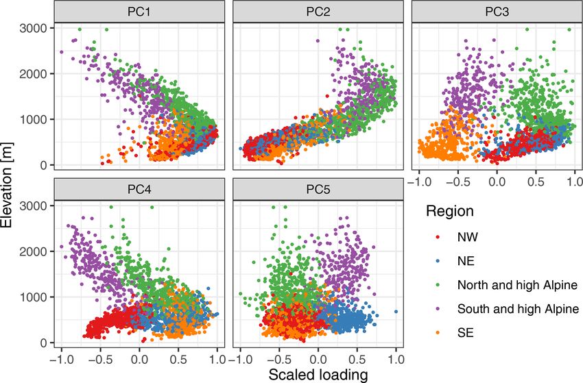
M. Matiu et al.: Observed snow depth trends in the European Alps: 1971 to 2019                                               1345

   The most relevant findings of the latest literature on snow      cal methods, Sect. 3 presents results and discusses them, and
cover trends (Table B1) can be summarized as follows. Snow          Sect. 4 provides conclusions.
variables exhibited a strong temporal and spatial variability
(e.g. Beniston, 2012b; Schöner et al., 2019). Long-term anal-
yses identified periods of high snow cover in the 1940s/50s,        2     Data and methods
as well as in the 1960s/70s, followed by absolute minima in
                                                                    2.1    Study region
the 1980s and early 1990s with some recovery afterwards
but not to the pre-1980s values (Marty, 2008; Micheletti,           The European Alps extend with their arc-shaped structure
2008; Scherrer et al., 2013; Schöner et al., 2009; Valt and         over more than 1000 km from the French and Italian Mediter-
Cianfarra, 2010). Trends were strongly related to elevation         ranean coasts to the lowlands east of Vienna, covering south-
(Laternser and Schneebeli, 2003; Marcolini et al., 2017b;           eastern France, Switzerland, northern Italy, southern Ger-
Valt et al., 2008) and were mostly negative at low eleva-           many, Austria, and Slovenia (see Fig. 1a). The Alpine region
tions (Bach et al., 2018), while higher elevations showed           is characterized by a very complex orography with large el-
no change or even increases (Marty et al., 2017; Terzago            evation gradients and deep valleys of different orientations
et al., 2010). Snow melt was identified as the main contribu-       intersecting the ridge and shaping numerous mountain mas-
tion to the decreasing trends (Klein et al., 2016), which ex-       sifs.
plains the pronounced trends at low elevations and in spring           Regarding their climatic setting, the European Alps are lo-
(Marty et al., 2017). Finally, after accounting for elevation,      cated in a transitional area influenced by the intersection of
regional differences between trends were observed (Benis-           three main climates: the zone impacted by the Atlantic Ocean
ton, 2012b; Laternser and Schneebeli, 2003; Schöner et al.,         with moderate wet climate, the zone linked to the Mediter-
2019; Terzago et al., 2013).                                        ranean Sea characterized by dry summers and wet and mild
   Quantitatively synthesizing all these studies into a com-        winters, and the zone characterized by European continental
mon Alpine view is challenging, and thus the provision of           climate with dry and cold winters and warm summers. Eleva-
quality-ensured information on snow cover climatology and           tional effects and very small-scale climatic features originat-
trends at larger extents, such as the whole Alpine mountain         ing from the complex Alpine topography are superimposed
range, is hampered (Hock et al., 2019). The challenge starts        on this large-scale climatic setting (Auer et al., 2005; Isotta
from the different definitions of the studied seasons, which        et al., 2014).
range from December–February to October–May, and thus                  The interaction of the three climate forcing zones, together
sometimes include the start, middle, and end of the season.         with the topography of the Alps, results in climatic gradients
Difficulties also arise in the selection of existing snow vari-     along the north–south and west–east directions. The intersec-
ables and indices, such as mean snow depth, maximum snow            tion of these two gradients can be characterized by four main
depth, snow days (based on thresholds from 1 to 50 cm), 3 d         climate regions, as shown by Auer et al. (2007). The first and
cumulative values, etc. Naturally, the station series are of dif-   sharpest climatic border is along the central main ridge sepa-
ferent lengths, and the studied periods get longer for the more     rating the temperate westerly from the Mediterranean sub-
recent studies. Finally, the statistical methods differ from        tropical climate. The second climatic border separates the
one study to another: linear regressions, Mann–Kendall tests,       western oceanic from the eastern continental influences.
Sen slopes, moving window approaches (windows ranging
from 5 to 20 years), breakpoint analysis, principal component       2.2    Data sources
analysis/empirical orthogonal function analysis (PCA/EOF),
and more.                                                           The acquisition of snow observation data was performed
   To overcome these limitations, we embarked on the effort         by using open data portals and by directly contacting data
to collect and analyse an Alpine-wide dataset of snow mea-          providers (see Table 1 for an overview). For Austria, the
surements from stations covering Austria, France, Germany,          Austrian Hydrographical Service (HZB, Hydrographisches
Italy, Slovenia, and Switzerland. The main aim is to under-         Zentralbüro) offers free downloads of their data for recent
stand how changes in snow cover vary over space and time by         decades, and additional historical data at the seasonal scale
applying the same methods to an as homogenous as possible           were kindly provided by the HZB. For France, data were
Alpine-wide dataset. This approach avoids sub-regional per-         kindly provided by the national weather service Météo-
spectives, inconsistencies from single data sources and dif-        France. This includes data collected as part of the collabora-
ferent methods, and influences of artificial boundaries such        tive network (réseau nivo-météorologique) between Météo-
as national borders. Since we wanted the data collection ef-        France and mountain stakeholders (in particular Domaines
fort to be of use for the scientific community, we make as          Skiables de France, Association Nationale des Maires des
much of the data as possible openly accessible (as far as data      Stations de Montagne, and l’Association Nationale des Di-
policies allow us to). The remainder of the paper is struc-         recteurs de Pistes et de la Sécurité de Stations de Sports
tured as follows: Sect. 2 introduces the data and the statisti-     d’Hiver). For Germany, data were downloaded from the
                                                                    national weather service’s (DWD, Deutscher Wetterdienst)

https://doi.org/10.5194/tc-15-1343-2021                                                   The Cryosphere, 15, 1343–1382, 2021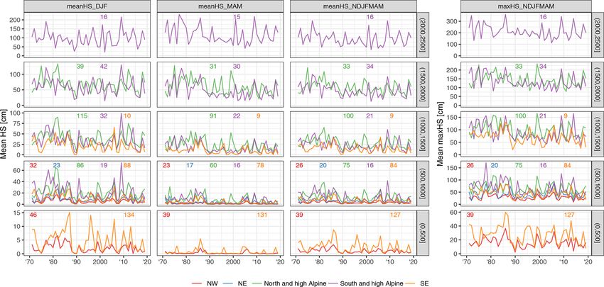
1346 M. Matiu et al.: Observed snow depth trends in the European Alps: 1971 to 2019
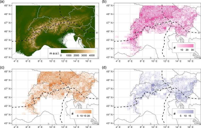
Figure 1. Topography of the European Alps (a) and overview of station locations (b–d). Panel (a) shows the SRTM30 DEM (Shuttle Radar
Topography Mission digital elevation model) with ∼ 1 km resolution. Panel (b) shows the location of snow depth measurement locations that
were available (provided). Panel (c) shows the locations of stations used in the regionalization analysis. Panel (d) shows the stations used for
the long-term trend analysis. The station density for a 0.5◦ × 0.25◦ grid is shown underneath the points in (b–d). The main climatic divides
from Auer et al. (2007) are shown as dashed lines in (a–d). See also Appendix A and Sects. 2.4 and 2.5 for selection criteria.
Table 1. Overview of the number of stations with daily data provided by the different data sources. The data source consists of a country
abbreviation, followed by the data source. Country abbreviations are AT for Austria, CH for Switzerland, DE for Germany, FR for France, IT
for Italy, and SI for Slovenia. For source abbreviations, please see Sect. 2.2. Station numbers are shown for depth of snowfall (HN) and snow
depth (HS) time series. See Appendix A and Sects. 2.4 and 2.5 for more details on station selection procedures associated with the different
types of analyses. HN was not analysed but was used for checking HS.
Data source HN HS HS used (regionalization) HS used (trend analysis)
AT_HZB 653 652 588 335
CH_METEOSWISS 505 501 142 79
CH_SLF 96 96 94 84
DE_DWD 956 964 830 104
FR_METEOFRANCE 239 286 145 45
IT_BZ 60 64 48 0
IT_FVG 30 30 18 8
IT_LOMBARDIA 11 11 11 0
IT_PIEMONTE 34 34 24 15
IT_SMI 6 8 8 7
IT_TN 52 52 29 8
IT_TN_TUM 0 5 1 0
IT_VDA_AIBM 57 57 17 5
IT_VDA_CF 0 17 11 3
IT_VENETO 10 11 11 9
SI_ARSO 130 172 172 152
Total sum 2839 2960 2149 854
The Cryosphere, 15, 1343–1382, 2021 https://doi.org/10.5194/tc-15-1343-2021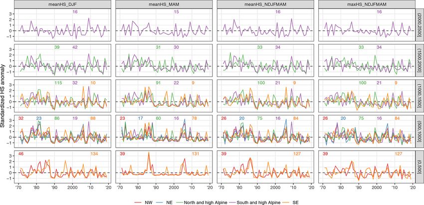
M. Matiu et al.: Observed snow depth trends in the European Alps: 1971 to 2019                                              1347

open data portal using the R package rdwd. For Germany,           or network, the observation modalities are remarkably simi-
only stations below 49◦ N were downloaded. For Italy, the         lar, thus allowing a combination of the different sources. For
data were kindly provided by many regional authorities:           more detailed information on the measuring modalities, we
                                                                  refer to the European Snow Booklet (Haberkorn, 2019). Val-
  – for the province of Bolzano, from the hydrographical          ues of HS and HN were rounded to full centimetres. The
    office of Bolzano (BZ);                                       further processing, quality checking, and gap filling are de-
                                                                  scribed in Appendix A. For all the following statistical anal-
  – for Friuli Venezia Giulia (FVG), from the regional
                                                                  yses, the processed and gap-filled data were used.
    weather observatory (OSMER, Osservatorio meteoro-
                                                                     The fraction of stations used from the MeteoSwiss data is
    logico regionale), which is part of the ARPA (Agen-
                                                                  very low compared to the other networks. The MeteoSwiss
    zia regionale per la protezione dell’ambiente) FVG and
                                                                  data contain a large number of stations from the manual pre-
    from where the data were collected and cleaned by the
                                                                  cipitation network which is not dedicated to snow. Many sta-
    Servizio foreste e corpo forestale struttura stabile cen-
                                                                  tions contain an important data gap for the 1981–1997 period
    trale per l’attività di prevenzione del rischio da valanga;
                                                                  that rendered a large fraction of the stations unusable for this
  – for Lombardy, from the ARPA Lombardia;                        study.
                                                                     The homogenization of series, which is the removal of
  – for Piedmont, from the ARPA Piemonte;                         non-climatic parts in the time series, such as, for example,
                                                                  those caused by instrumentation changes or station reloca-
  – for the province of Trento, from Meteotrentino (TN)           tions, is a standard practice in long-term temperature and
    with some additional long-term series previously anal-        precipitation records (Auer et al., 2007). Applying the same
    ysed (TN_TUM; Marcolini et al., 2017a);                       tools to snow depth is not straightforward. There is an ongo-
                                                                  ing discussion on the appropriate homogeneity tests and suit-
  – for the Aosta Valley (VDA), from the civil protection         able observation frequency, such as daily, monthly, or sea-
    office (CF: Centro funzionale, Regione Valle d’Aosta)         sonally (Marcolini et al., 2017a, 2019; Schöner et al., 2019).
    and from the avalanche office (AIBM: Assetto idrogeo-         An analysis of a dataset with parallel snow measurements in-
    logico dei bacini montani, Regione Valle d’Aosta);            dicates that snow cover duration and maximum snow depth
                                                                  are amongst the indicators least affected by inhomogeneities
  – for Veneto, from the avalanche office (Centro valanghe
                                                                  (Buchmann et al., 2021). Current research has tried to ex-
    di Arabba), which is part of the ARPA Veneto;
                                                                  tend existing approaches with new innovations (Resch et al.,
  – and, finally, additional data for Piedmont and Aosta Val-     2020). Homogenization could improve the robustness of es-
    ley from the Italian meteorological society (SMI, Soci-       timated trends, and be especially useful for areas with sparse
    età Meteorologica Italiana).                                  observations, such as for elevations above 2000 m. Given the
                                                                  large extent of our dataset, it was not possible to apply a com-
For Slovenia, data were kindly provided by the Slovenian En-      mon homogenization framework for our study, and we leave
vironmental Agency (ARSO, Agencija Republike Slovenije            this for future studies.
za okolje). For Switzerland, data were downloaded from the
IDAWEB portal of the national weather service MeteoSwiss,         2.3   Data overview
and additional data were kindly provided by the WSL In-
stitute for Snow and Avalanche Research SLF. This dataset         The locations of the stations are shown in Fig. 1b–d, the
comprises the entire geographical range of the European           availability of stations in time in Fig. 2a, and the elevational
Alps, yet we are aware of the existence of additional datasets    distribution in absolute terms in Fig. 2b and in relative terms
(such as in the private sector or public but not yet digitized)   in Fig. 2c. The stations cover the whole Alpine arc, but they
which unfortunately were not included in this analysis and        are distributed with different station densities arising from
whose inclusion would be beneficial for even more robust          the different national and regional networks. As expected,
results.                                                          most stations were found at lower elevations, the maximum
   The data consist of daily measurements of snow depth           number was at ∼ 500 m, and the number sharply declined at
(HS) and depth of snowfall (HN). The largest part of the          higher elevations. Above 2000 m, the number was low, and
data is manual measurements. Some automatic measure-              no stations above 3200 m were available for this study. The
ments were included in the dataset provided for France. For       longest series dates back to the late 19th century for HS (Pas-
a few sites in the Aosta Valley in Italy, manual series were      sau Maierhof in Germany, starting in 1879). The total number
merged with automatic series. This was done in order to ex-       of available HS stations depended on the availability of dig-
tend up to the present some records that were dismissed at        itized data. It slowly started increasing around ∼ 1900 with
the beginning of the last decade, and this was performed in       significant jumps in the 1960s and 1970s when the French,
close communication with the operating office. While the ob-      Slovenian, and Austrian series started and in the 1980s when
servers follow slightly different guidelines in each country      Germany had a large network increase. The highest number

https://doi.org/10.5194/tc-15-1343-2021                                                The Cryosphere, 15, 1343–1382, 2021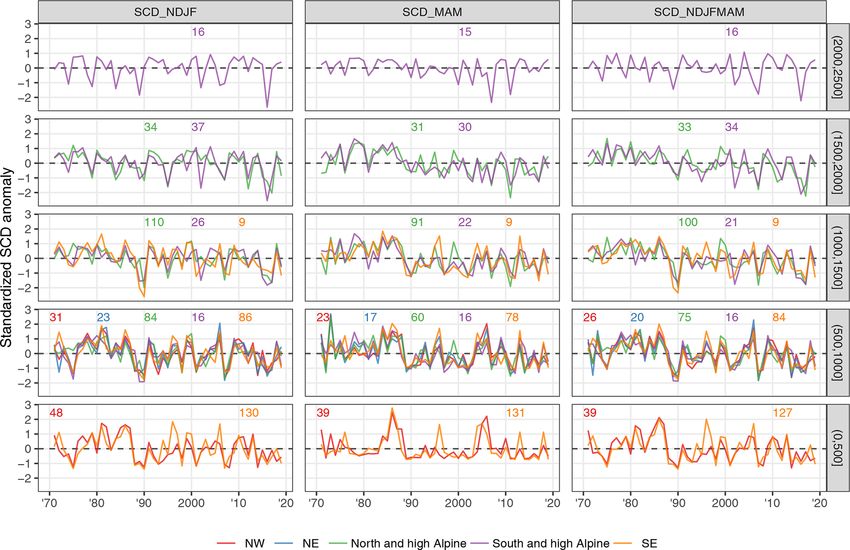
1348                                         M. Matiu et al.: Observed snow depth trends in the European Alps: 1971 to 2019

Figure 2. Overview of temporal data availability and station elevation. (a) The number of stations with daily data (before gap filling) is
shown per year and country, as well as a total sum for the whole Alpine region. Stations are included in the count if they have at least one
non-missing observation in the respective calendar year. This simple threshold was chosen because the aim of this figure is to show the
availability and network abundance. Country abbreviations are like in Table 1. (b) The elevational distribution of snow depth (HS) stations in
absolute numbers. For the histogram, 50 m bins were used. (c) Comparison of the relative elevational distribution of the station locations vs. a
digital elevation model (DEM). The distribution of the stations is shown in relative terms using the same bin width (50 m) as in the histogram
in (b) but normalized to show the relative frequency instead of absolute numbers and displayed as lines instead of bars. This is compared to
the elevation for the whole area spanned by the stations (see polygon in inset map; area was outlined manually along the stations), which is
extracted from the SRTM30 DEM (Shuttle Radar Topography Mission; ∼ 1 km resolution).

of stations was available after the 1980s with approximately              2.4    Regionalization
2000 stations. The total number of stations dropped signif-
icantly after 2017 because the data for Austria were only
available until 2016 due to the delays caused by the data                 An empirical orthogonal function (EOF) analysis, also called
provider performing quality checks. Moreover, the data col-               principal component analysis (PCA), was conducted to de-
lection was performed between 2019 and 2020, thus some                    termine the common modes of spatial variability. PCAs are
sources ended in between. We used two different periods for               widely employed in climatological studies to evaluate spa-
the two analyses that we performed. For the regionalization,              tial modes of variability (Storch and Zwiers, 1999). They
we aimed to have the largest possible spatial extent and den-             have been employed for meteorological records in the Eu-
sity of the stations; so the period 1981 to 2010 was chosen               ropean Alps (Auer et al., 2007) and also for snow variables
because it is the period with the highest number of stations.             (López-Moreno et al., 2020; Scherrer and Appenzeller, 2006;
For the trend analysis, we aimed to have trends as long as                Schöner et al., 2019; Valt and Cianfarra, 2010). For the PCA,
possible that sample the whole region; so the period 1971 to              we used daily quality-checked and gap-filled data. However,
2019 was chosen because it offered the best tradeoff between              the gap filling was only employed when enough confidence
station coverage and period length.                                       in the filled value could be expected (see Appendix A for
                                                                          a detailed description), so some of the series still had gaps.
                                                                          Because the aim of this regionalization was to have a large
                                                                          spatial coverage, we did not want to exclude series with only

The Cryosphere, 15, 1343–1382, 2021                                                             https://doi.org/10.5194/tc-15-1343-2021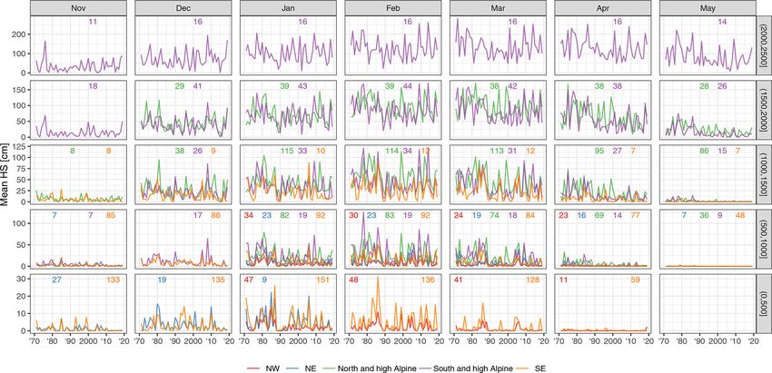
M. Matiu et al.: Observed snow depth trends in the European Alps: 1971 to 2019                                                      1349

a few missing values. Consequently, we used a modification             the snow season: monthly mean HS for November to May,
of the PCA algorithm that allows for the use of data with gaps         mean winter HS (December to February, DJF), mean spring
to estimate the principal components (Taylor et al., 2013).            HS (March to May, MAM), mean seasonal HS (November
   The PCA was applied to the daily data from December to              to May), maximum HS from November to May (maxHS),
April for the hydrological years 1981 to 2010. The period              early season snow cover duration (SCD, November to Febru-
was chosen because it is long enough to provide a climato-             ary), late season SCD (March to May), and full season SCD
logical reference (30 years), and it is the period that has the        (November to May). SCD was the number of days with HS
largest number of stations available. A hydrological year is           above 1 cm (Brown and Petkova, 2007). Indices were cal-
defined here as starting in October, and it is designated as           culated from the quality-checked and gap-filled daily snow
the calendar year of the ending month (e.g. December 1998              depth observations if more than 90 % of the daily values in
to April 1999 belong to the hydrological year 1999). Only              the respective period were available. Trends of all indices
those stations were selected that had at least 70 % of daily           were calculated for the period 1971 to 2019 for stations with
data available in this period. Each series was scaled to zero          complete data in the period. For the monthly mean HS analy-
mean and unit variance before applying the PCA.                        sis only, April and May series displaying mean HS less than
   In order to identify spatially homogeneous regions within           1 cm in all years were discarded because these are insignif-
the Alpine domain, we performed a k-means clustering on                icant snow amounts which divert attention from the other
the estimated PCA matrix. We tested configurations with                sites; series of the other months at the site were still included.
two to eight clusters with the PCA matrix and with two to              The number of series available for each snow variable differs;
eight principal components (PCs) as input. We also applied             the largest number of series is available for the monthly mean
k-means clustering directly on scaled daily observations of            HS, less for the half-seasonal (3 to 4 months) indices, and the
snow depth for comparison. To identify the best number of              fewest for the full-season indices.
clusters, we used the “elbow method”, average silhouette co-              Trend analysis was performed using generalized least
efficients, and visual interpretation. For the elbow method,           squares (GLS) regression. GLS was used because it allows
the fraction of explained variance is plotted against the num-         for changes in the variance to be accounted for (Pinheiro
ber of clusters, and the elbow of this curve is the point where        and Bates, 2000). This was employed because the monthly
the increase in explained variance becomes marginal. This              snow depth series exhibited a change in the interannual vari-
is a semi-objective method because an elbow cannot always              ability, especially at the end of the season when monthly
be clearly identified. The silhouette is a measure of how              snow depths approached zero. The regression formula was
well an observation fits into its own cluster vs. the others.          yt = β0 + β1 t + t , where yt is the value of the respective
For an observation i in cluster Ci , the silhouette coefficient        snow variable in year t (centred such that year 1971 becomes
is 1 − a(i)/b(i) if a(i) < b(i), b(i)/a(i) − 1 if a(i) > b(i)          year 0), β0 and β1 are the estimated regression coefficients,
and 0 if a(i) = b(i), where a(i) is the mean distance be-              and t is the normally distributed errors with mean zero.
tween i and all other points in the same cluster, and b(i) is          GLS allows for the variance to depend on the year t with
the smallest mean distance of observation       i to all other clus-   Var(t ) = σ 2 · exp(2 · γ · t), where γ is a coefficient to be es-
ters. Specifically, a(i) = |Ci1|−1 j Ci ,i6=j d(i, j ) and b(i) =
                                   P
                                                                       timated in the inference procedure that indicates the change
mink6=i |C1k | j Ck d(i, j ), where d(ij ) is the Euclidean dis-
              P                                                        in variance associated to t. The GLS regressions for monthly
tance between observations.                                            mean HS showed a significantly improved goodness of fit
   The optimal number of clusters varied between two and               (p < 0.05, likelihood ratio test) for 40 % of all cases and,
five depending on the input (observations or PCA matrix)               specifically for November, April, and May, even for more
and depending on the metric (elbow in variance explained               than 60 % when compared to ordinary least squares (OLS)
or average silhouette coefficients). Additional PCs only ex-           that assumes a constant error variance. The significance of
plained less than 2.6 % of the variance. After looking at the          trends was assessed using a 95 % confidence level. For the
clustering results on maps (see Fig. S1 in the Supplement),            fraction of the variance explained by the trend, we used the
all two to five clusters are meaningful. They simply highlight         R squared statistic. To determine the magnitude of the inter-
different aspects of the snow depth spatial variability, such          annual variability after accounting for the trend, we used the
as the gradients along elevation, north–south, and west–east.          standard deviation (SD) of the model residuals.
Finally, five clusters based on the PCA matrix were chosen                An alternative for dealing with such heteroscedastic data
because they provide the best trade-off between the semi-              is to use the robust nonparametric Theil–Sen trend estima-
objective metrics and the patterns expected from the climatic          tor with the Mann–Kendall test for significance assessment.
drivers.                                                               We systematically evaluated the differences in the estimated
                                                                       trend magnitudes and trend significance of the Theil–Sen ap-
2.5   Trend analysis                                                   proach vs. the GLS model and found only negligible differ-
                                                                       ences (Fig. S13 and Table S10 in the Supplement); the mean
For the trend analysis, monthly and seasonal indices were              difference between trend estimates was 0.02 cm per decade,
used which are indicative for different aspects and times of           the correlation between trend estimates was 0.96, and the

https://doi.org/10.5194/tc-15-1343-2021                                                       The Cryosphere, 15, 1343–1382, 2021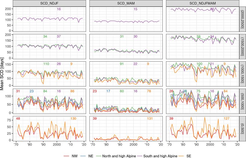
1350                                      M. Matiu et al.: Observed snow depth trends in the European Alps: 1971 to 2019

agreement of significance based on a p value threshold of          6 h for temperature from MESCAN-SURFEX) series were
0.05 was 86 %.                                                     aggregated to monthly means for temperature and monthly
   The SCD variables are bounded counts which can pose             sums for precipitation.
problems to the assumption of standard linear regression with         The gridded products have a reference orography that, in
normally distributed errors. This was only problematic for         complex mountain terrain, can differ significantly from the
very low- and very high-elevation sites which display many         elevation of the point observation, thus, for example, intro-
SCD values at the minimum or maximum. For MAM, this                ducing biases in temperature. Hence, temperatures were ad-
concerns series below 500 m and above 2000 m, while for            justed using a constant lapse rate of 6.5 ◦ C km−1 .
November–February (NDJF) and November–May (NDJF-                      Monthly temperature and precipitation can be considered
MAM), this is problematic below 250 m and above 2500 m.            largely independent from one month to the next, while snow
Instead, for such count data, a probability distribution such as   cover is a cumulative process across the snow season. Be-
negative binomial would be more appropriate (Venables and          cause of this, seasonal comparisons were performed with av-
Ripley, 2002). Compared to the Poisson distribution, the neg-      erage seasonal temperature and precipitation for winter (De-
ative binomial family accounts for overdispersion. We evalu-       cember to February), spring (March to May), and the whole
ated the differences in trend estimates and trend significance     snow season (November to May). The time period 1981 to
between the negative binomial linear model and the GLS             2010 was used, which had the densest station coverage. Cli-
model. Since the negative binomial linear model gives rel-         matological averages were computed for all seasons using
ative estimates of trends, these were transformed to absolute      the quality-checked and gap-filled snow depth data. Since
decadal trends for comparison. Again, differences were neg-        EURO4M-APGD ends in 2008, the time period 1981 to 2008
ligible on average (Fig. S13 and Table S10). Consequently,         was used for the observation-based products. The paper con-
we applied the GLS model for all snow variables.                   tains results from the comparison with the reanalysis product
                                                                   (MESCAN-SURFEX), and the results from the observation-
2.6    Air temperature and precipitation data                      based products are shown in the Supplement as a sensitivity
                                                                   analysis.
In order to study the relationship of snow depth with tem-
perature and precipitation, we extracted temperature and pre-
cipitation series for each station from available gridded prod-    3     Results and discussion
ucts. While gridded datasets clearly have some shortcomings,
e.g. comparisons with point observations need a cautious in-       3.1    Regionalization of daily snow depths 1981 to 2010
terpretation (Salzmann and Mearns, 2011), their strength is
the spatial and temporal coverage.                                 The PCA of daily snow depth series yielded five main modes
   Two types of products were considered. The first is a re-       of spatial variability which explained in total 84 % of the
analysis, and the second is an observation-based spatial anal-     variance in the period December to April from 1981 to 2010
ysis. For the reanalysis, we used temperature and precipi-         (Fig. 3). The first PC explained 54.3 % of the variance and
tation from the MESCAN-SURFEX dataset (Bazile et al.,              distinguished between high- to middle- and low-elevation
2017) which was produced during the UERRA (Uncertain-              stations (approximate threshold 500–1000 m; Fig. 4). It ex-
ties in Ensembles of Regional Reanalyses) project and which        plained the variability in snow depth for stations above
is available via the Copernicus Data Store (CDS). It covers        1000 m and was probably also partly linked to the perma-
the period from January 1961 to July 2019 on a 5.5 km grid.        nence (or permanent absence) of snow cover, which is also
Precipitation is available as total daily sum and temperature      why some low-elevation sites presented similar loading to the
at 6 h intervals (00:00, 06:00, 12:00, 18:00 UTC). For the         high sites (a PC loading can be considered the correlation of
observation-based data, we chose E-OBS v20.0e for mean             the original series with the principal component). The second
daily temperature (Cornes et al., 2018) and the Alpine pre-        PC explained 11.9 % of the variance and was also linked to
cipitation grid dataset (EURO4M-APGD) for total daily pre-         elevation, but it captured the variability below 1000–1500 m
cipitation (Isotta et al., 2014; Isotta and Frei, 2013). E-OBS     (Fig. 4). Consequently, PC1 and PC2 together captured the
v20.0e spans the period from January 1950 to July 2019 on          variability across the whole elevation range. The third PC ex-
a 0.1◦ grid. APGD covers the period from January 1971 to           plained 8.1 % of the variance and separated the stations into
December 2008 on a 5 km grid. It should be noted that the          north and south of the main ridge. The fourth PC explained
observation-based precipitation grids do not account for un-       6.0 % of the variance and separated the stations into east from
dercatch, which can lead to uncertainties at high elevations       west. The fifth PC explained 3.7 % of the variance and sep-
and in winter (Prein and Gobiet, 2017).                            arated the south-eastern and north-western stations from the
   In order to assign grid cells to stations for temperature and   rest.
precipitation, we selected those grid cells which contain the         Some gradients in the PC loading map (Fig. 3) could give
stations. Consequently, some nearby stations could have the        the impression that data artefacts between the different data
same series of temperature and precipitation. The daily (or        providers exist, such as at the Austrian–German border in

The Cryosphere, 15, 1343–1382, 2021                                                   https://doi.org/10.5194/tc-15-1343-2021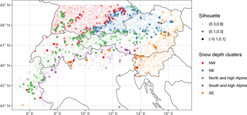
M. Matiu et al.: Observed snow depth trends in the European Alps: 1971 to 2019                                                         1351

Figure 3. Main modes of variability in daily snow depth series. The plots show scaled loadings for the first five principal components (PCs),
which can be considered the correlation of the original series with the respective PC. The title in each panel contains the amount of the
variance explained by the respective PC. The principal component analysis was applied to daily snow depth data from December to April for
the hydrological years 1981 to 2010 for stations that had at least 70 % of available data.

Figure 4. Scatterplots of principal component (PC) loading vs. elevation and region. The PC loading can be considered the correlation of the
original series with the respective PC. See Fig. 3 for a map of the PC loadings and Fig. 5 for a map of the regions.

PC2 and PC5 or at the French–Italian border in PC3-5. How-               of 472 m (min–max: 30–1510 m), which contained stations
ever, this is caused by the fact that the administrative borders         from south-western Germany, north-western Switzerland, a
in the Alps are tied to topography and thus closely located              few from France, and a few from eastern Austria; north-east
near elevational borders (Fig. 1a). A version of Fig. 3 sub-             (NE) with a median elevation of 515 m (215–1188 m), which
divided by data provider highlights clearly that the gradients           contained stations from south-eastern Germany and north-
were not associated with the administrative borders (Fig. S2             ern Austria; and north and high Alpine with a median el-
in the Supplement).                                                      evation of 1050 m (482–2970 m), which contained stations
   The PCA loadings from the five PCs were used as input for             mainly located in France, Switzerland, and Austria but also
a clustering algorithm (k means) which divided the stations              includes the high-elevation sites in Germany, such as in the
into five clusters or regions (Fig. 5). This yielded three re-           Black and Bavarian forests. Two regions emerged south of
gions in the north: north-west (NW) with a median elevation              the main ridge: south and high Alpine with a median el-

https://doi.org/10.5194/tc-15-1343-2021                                                         The Cryosphere, 15, 1343–1382, 2021
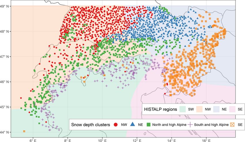
1352                                       M. Matiu et al.: Observed snow depth trends in the European Alps: 1971 to 2019

Figure 5. Clustering of stations based on daily snow depth data. Map of regions from applying a k-means clustering on the first five prin-
cipal components. Underlaid are the HISTALP coarse-resolution subregions (Auer et al., 2007) which were derived using a semi-automatic
principal component analysis of climate variables (temperature, precipitation, air pressure, sunshine, and cloudiness).

evation of 1530 m (588–2735 m), which contained stations               data since the results looked almost identical to a standard
from the southern French Alps, almost all of Italy, a few in           PCA (see Figs. S3 and S4 in the Supplement), in which the
southern Switzerland, and some in southern Austria and east-           clustering agreed in 98.5 % of the stations, and the same sta-
ern Slovenia; and south-east (SE) with a median elevation of           tions seemed mis-clustered. Instead, this might be related to
420 m (55–1300 m), which contained almost all stations from            special local climatic conditions affecting snow cover or to
Slovenia and parts of eastern Austria.                                 the fact that these stations did not have any similar neigh-
   Consequently, clusters NW, NE, and SE contained lower-              bours in the estimated clusters. For example, the five stations
elevation sites, while north and high Alpine and south and             in Ticino, located in Switzerland south of the main ridge,
high Alpine contained the higher elevations. The spatial cov-          are low-elevation stations that had no correspondence in the
erage of the stations in this study included low-elevation sites       south and high Alpine cluster which is comprised of mid-
for Switzerland, Germany, Austria, and Slovenia but not for            dle to high elevations. Thus, the next best clusters were the
France and Italy where the available stations were mostly              SE and NW which, however, did not fit well; these sites and
high-elevation sites. For future analysis, it would be inter-          all other seemingly mis-clustered stations had low silhouette
esting to include more low-elevation sites from France and             values (Fig. B1), which is a measure of how well a point
Italy and see whether a third cluster would emerge (as in the          matches its cluster compared to the others. Low silhouette
north) because the division into south and high Alpine and             values were also found along the borders of the different
SE is surely also caused by the different station elevations.          clusters, especially between NW and NE, which implies a
   The results from the clustering were obtained automati-             smoother transition between NW and NE compared to the
cally, and no manual post-processing or modification of the            north–south boundary.
cluster assignments was performed. Additionally, the only                 The estimated modes of variability in snow are similar
input into the clustering algorithm was daily snow depth               to previous estimates on climatic subregions in the Alps, as
series, and no information on location or elevation was in-            identified in the HISTALP project (Auer et al., 2007) and
cluded. Given this absence of location information in the              which are underlaid in Fig. 5. The HISTALP regions were
clustering process, the estimated modes of variability and the         based on temperature, precipitation, air pressure, sunshine
resulting regions were very homogenous in space. However,              and cloudiness, and the division into north, south, east, and
in the clustering, some stations seemed off, such as the few           west matches what we found for snow depth. Since the four
north-west stations around Lugano in Switzerland, northern             regions were a compromise between all variables, they do
Italy, and on the Adriatic coast in Slovenia, as well as the SE        not match perfectly to what we found for snow depth because
stations in France, Switzerland, and northern Italy. This was          the individual atmospheric variables exert different controls
not related to the PCA algorithm used that allowed gaps in             on surface snow cover. While the north–south boundary is al-

The Cryosphere, 15, 1343–1382, 2021                                                         https://doi.org/10.5194/tc-15-1343-2021
M. Matiu et al.: Observed snow depth trends in the European Alps: 1971 to 2019                                                1353

most identical in the central-western part, the eastern part has   much higher variability than temperature. Correlations of
large mismatches. However, if the single element boundary          snow depth with temperature did not differ by region. How-
for precipitation was considered as a main factor (cf. Fig. 8      ever, the stations in the SE exhibited stronger (more positive)
from Auer et al., 2007), then the agreement with snow depth        correlations with precipitation than the NE and NW regions.
would be almost perfect. This finding confirms a consistent           The findings on the correlations agree with previous esti-
picture of the Alpine climate in which snow depth is strongly      mates for Swiss and Austrian stations (Schöner et al., 2019)
related to precipitation and air temperature patterns.             in terms of signs and elevation patterns. However, our esti-
   The amount of the variance explained in the PCA with five       mates are of higher magnitude for both temperature and pre-
PCs (84 %) might seem surprisingly high given that snow            cipitation. As a sensitivity analysis, we repeated the climatol-
cover is hypothesized to have a high spatial and temporal          ogy and correlational analysis using observation-based spa-
variability. The value is higher than recent estimates for the     tial analyses instead of reanalysis for extracting temperature
Swiss Alps, where the first three PCs explained 78 % of the        and precipitation (Figs. S6 and S7 and Tables S3 and S4 in
snow cover (Scherrer and Appenzeller, 2006), or for Austria        the Supplement), but results did not differ substantially from
and Switzerland, where the first three PCs explained 70 %          above.
of the snow cover (Schöner et al., 2019). However, since we
included here more stations and also stations from regions
                                                                   3.3   Long-term trends for the period 1971 to 2019
with different climatic influences, such as south of the main
ridge, an increase in the amount of the explained variance
could be expected.                                                 Trends of monthly mean snow depth from November to May
                                                                   were mainly negative with some exceptions (Fig. 7 and Ta-
3.2   Snow depth climatology 1981 to 2010 and links to             ble 2). Over all stations and all months, 85 % of the trends
      temperature and precipitation                                were negative and 15 % positive; 23 % were significantly
                                                                   negative and 0 % (only four station–month combinations)
Besides differences in the patterns of daily variability in the    significantly positive (for significance, p values had to be less
snow depth series, the regions also demonstrated different         than 0.05). The percentage of significant negative trends was
snow depth climatologies (Fig. 6). Looking at average winter       substantially higher in the spring months (March to May) and
(December to February) snow depth from 1981 to 2010, the           at lower elevations irrespective of region, and it could reach
northern regions had higher snow depths than their southern        40 %–70 % (see also Table 2).
counterparts. These differences became larger with increas-           In the low-elevation regions (NE, NW, SE), snow depth
ing elevation. While below 750 m no substantial differences        was decreasing much stronger in the SE than in the NE or
were observed, southern stations had ≈ 30 % less snow than         NW across all months. The mean trend of December snow
northern stations until 1750 m and ≈ 20 % less until 2250 m;       depth below 1000 m in the NE was −0.7 cm per decade (all
above this the number of stations is too low to obtain robust      further trends in the same unit) and −0.8 in the SE, while in
results (Table S1).                                                January, it was −0.5 in the NW, −0.6 in the NE, and −1.6
   Average winter temperatures were higher in the NW com-          in the SE (Table 2). In February, NE stations even had an in-
pared to the NE and SE, and the latter two were similar. In        creasing snow depth at +0.8, while in the NW and SE it de-
north and high Alpine and south and high Alpine, temper-           creased. At middle elevations (1000 to 2000 m), differences
atures were also comparable, although northern sites were          between north and south were even stronger and variable in
colder at 1500–2000 m. However, precipitation amounts              amplitude during the snow season; in December, the mean
were significantly lower in the south than north, and south        trend in north and high Alpine (N&hA) stations was more
and high Alpine sites received ≈ 100 mm less winter precip-        strongly negative (−1.9) compared to south and high Alpine
itation than north and high Alpine sites up to 2000 m, which       (S&hA) stations (−0.8), but for January and February, we
amounts to ∼ 1/3 of the precipitation in the north. These re-      observe the opposite behaviour with a less pronounced neg-
sults suggest that the difference in the December to February      ative trend in N&hA (−1.6 and −2.2) compared to S&hA
snow amounts in the north vs. south is predominantly driven        (−3.9 and −5.1).
by precipitation differences and not temperature.                     In the spring months of March and April, trends in snow
   Seasonal snow depth was correlated to temperature and           depth were again more negative in the south than north. For
precipitation extracted from a gridded reanalysis (MESCAN-         example, at middle elevations (1000 to 2000 m), the mean
SURFEX). Results indicated negative correlations with tem-         March snow depth trend was −3.9 in N&hA compared to
perature decreasing strongly with elevation and positive cor-      −7.0 in S&hA, in April −5.7 compared to −6.6, and in May
relations with precipitation mildly increasing with elevation      −1.4 compared to −2.7. Notably, stations in S&hA above
(Fig. S5 in the Supplement). The magnitude of temperature          2000 m exhibited strong variability in trends, and there were
correlations was between −0.8 and −0.5 below 1000 m, and           stations with increasing snow depth in all months (Novem-
the correlation decreased to about −0.2 up to 2000 m. For          ber to May). While mean trends were positive until January
precipitation, correlations were between −0.2 and 0.7 with         (November 2.7, December 4.0, January 0.0), mean trends

https://doi.org/10.5194/tc-15-1343-2021                                                  The Cryosphere, 15, 1343–1382, 2021
1354 M. Matiu et al.: Observed snow depth trends in the European Alps: 1971 to 2019
Figure 6. Climatology of (a) snow depth, (b) temperature, and (c) precipitation across regions and elevations for the winter season (December
to February, DJF) and spring season (March to May, MAM). Average values are for the period 1981–2010. Each point represents one station.
The temperature and precipitation values were extracted from MESCAN-SURFEX reanalysis, while the snow depths are based on station
data. See also Tables S1 and S2 in the Supplement for summary values.
were negative otherwise (February −1.9, March −2.6, April different regions showed similar large-scale patterns, and, for
−8.3, May −9.5). example, the 1990s drop can be seen across the whole Alps.
Particular years, especially extreme ones, show concurrent
3.4 Interannual variability from 1971 to 2019 behaviour, for example February 1986 or 2009. Otherwise,
there is mixed coherence across regions, as can also be seen
Complementing the trend analysis, this section presents an from looking at standardized anomalies (Fig. B2) instead of
evaluation of the interannual variability in snow depth series. raw snow depth.
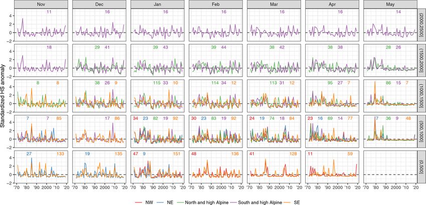
Figure 8 highlights that mean snow depth exhibited a strong These patterns are generally in line with those presented
interannual variability in the analysed period. Because of the in previous studies which showed high snow amounts in the
large number of stations, only time series that average over 1960s and 1980s and negative anomalies in the 1970s and
all stations in 500 m elevation bands are shown; however, in- 1990s, i.e. snow-scarce winters, regime shifts, or breakpoints
dividual station behaviour was well represented by the 500 m in that period in France, Switzerland, Italy, and the west-
averages; see also auxiliary plots in the repository (Matiu ern and southern part of Austria, and a recovery afterwards
et al., 2020). In the 1970s and 1980s, high snow depths were (Durand et al., 2009; Laternser and Schneebeli, 2003; Mal-
observed, followed by a period of extreme low snow depth lucci et al., 2019, 2019; Marcolini et al., 2017b; Marty, 2008;
in the 1990s. Since the 1990s, snow depths in winter have Micheletti, 2008; Scherrer et al., 2013; Schöner et al., 2019;
partly recovered, while in spring, snow depths have contin- Valt and Cianfarra, 2010). In an Alpine-wide view, this tem-
ued to decline. At the end of the snow season and for lower poral variability is also accompanied by a strong regional
elevations, average snow depths approached zero, such as in variability.
April for 500 to 1000 m or in May for 1000 to 1500 m. The
The Cryosphere, 15, 1343–1382, 2021 https://doi.org/10.5194/tc-15-1343-2021M. Matiu et al.: Observed snow depth trends in the European Alps: 1971 to 2019 1355 Figure 7. Long-term (1971 to 2019) linear trends in mean monthly snow depth (HS). Trends are shown separately by month (columns) and region (rows). Each point is one station. The points indicate the trend and the lines the associated 95 % confidence interval. In order to put the trends from Sect. 3.3 in the context of in- cant trends (p < 0.05) was 10 %. However, R 2 increased with terannual variability, we examined their relationship by look- elevation and in the last months of the snow season reached ing at the ratio between the 1971 to 2019 trend and the SD up to 32 %. of residuals (Fig. B3a). This gives an indication of the rela- From Fig. 8, a decrease in the variability in the snow depth tive contribution of the trend to interannual variability. The series can be observed, especially at the end of the season and highest ratios were observed in November to January below for lower elevations. This is confirmed by the large fraction 1000 m, in March between 500 and 2000 m, in April between of negative time coefficients for the error variance in April 0 and 2500 m, and in May between 1500 and 2500 m. and May (Table B2) in which approximately 40 %–80 % of As expected from the high temporal variability in the snow the stations presented significantly decreasing variability de- depth series, the fraction of explained variance from the lin- pending on the region. Notable decreases in variability were ear trends was low. The average R 2 over models with signifi- also observed in November and in January for the NE, NW, https://doi.org/10.5194/tc-15-1343-2021 The Cryosphere, 15, 1343–1382, 2021
1356                                         M. Matiu et al.: Observed snow depth trends in the European Alps: 1971 to 2019

Table 2. Overview of long-term (1971 to 2019) trends in mean monthly snow depth. Summaries are shown by month, region, and 1000 m
elevation bands (0 to 1000, 1000 to 2000, and 2000 to 3000 m). Cell values are the number of stations (#), the mean trend (mean, in centimetres
per decade), and percentages of significant negative (sig−) and positive (sig+) trends; the remaining percentage (not shown) corresponds
to the total of non-significant negative and positive trends. Empty cells denote no station available (for # and mean) and no stations with
significant negative or positive trends (sig− and sig+). Trends were considered significant if p < 0.05. See also Fig. 7. A version of the table
with 500 m bands instead of 1000 m is available in the Supplement (Table S5).

        Month     Region           Elevation: (0,1000] m              Elevation: (1000,2000] m              Elevation: (2000,3000] m
                               #     mean       sig−       sig+      #    mean       sig−     sig+      #      mean      sig−     sig+
        Nov       NW           2    −0.01     50.0 %
                  NE          34    −0.32     41.2 %
                  N&hA         4    −0.93     50.0 %                9    −0.31
                  S&hA         7    −1.02     71.4 %               23    −0.22                         12       2.68
                  SE         218    −0.50     52.3 %                8    −1.21     50.0 %
        Dec       NW           2    −0.01
                  NE          24    −0.68     29.2 %
                  N&hA         3    −1.72     33.3 %               67    −1.91      1.5 %               1     −2.02
                  S&hA        17    −1.34      5.9 %               67    −0.89      1.5 %     1.5 %    17      3.98
                  SE         221    −0.77     24.9 %                9    −2.38     44.4 %
        Jan       NW          81    −0.51     12.3 %
                  NE          32    −0.55      3.1 %                2     0.23
                  N&hA        83    −1.59      3.6 %              154    −1.59      4.5 %               4     −2.02
                  S&hA        19    −4.91     73.7 %               76    −3.94     21.1 %              17      0.50
                  SE         243    −1.59     29.6 %               10    −4.32     70.0 %
        Feb       NW          78    −0.09     11.5 %
                  NE          24     0.75                           1     2.44
                  N&hA        84    −1.36      4.8 %              153    −2.24      7.2 %               4     −3.56
                  S&hA        19    −4.10     10.5 %               78    −5.09     15.4 %              17     −1.91      5.9 %
                  SE         228    −0.63      4.4 %               12    −2.50
        Mar       NW          65    −0.33      4.6 %
                  NE          20    −0.93     10.0 %                1     0.10
                  N&hA        75    −3.10     30.7 %              151    −3.94     21.9 %               4     −1.91
                  S&hA        18    −3.52     33.3 %               73    −7.00     46.6 %              17     −2.55    11.8 %    5.9 %
                  SE         212    −0.65      5.2 %               12    −3.22     16.7 %
        Apr       NW          34    −0.08     23.5 %
                  NE          18    −0.33     38.9 %                1    −0.73
                  N&hA        69    −1.48     68.1 %              133    −5.70     65.4 %               4     −7.07    25.0 %
                  S&hA        14    −0.92     50.0 %               65    −6.63     56.9 %              17     −8.28    41.2 %
                  SE         136    −0.13     38.2 %     0.7 %      7    −1.42     14.3 %
        May       NE           7    −0.01
                  N&hA        36    −0.03      5.6 %              114    −1.42     28.1 %               3     −5.69
                  S&hA         9    −0.01     11.1 %               41    −2.68     39.0 %              15     −9.46    40.0 %
                  SE          52    −0.02                1.9 %      7    −0.02

and SE. Considerable significant increases in variability, on             seasonal indices of mean and maximum snow depth, as well
the other hand, were only observed in December for 27 % of                as snow cover duration (Tables 3 and 4; Appendix C). The
the south and high Alpine series.                                         results of seasonal mean HS agree with the monthly analy-
                                                                          sis and show generally decreasing snow depths in winter up
3.5    Seasonal snow indices of snow depth and snow                       to 2000 m and in spring for all elevations. Maximum snow
       cover duration                                                     depth across the whole season (November to May) decreased
                                                                          stronger than mean snow depth; e.g. the average trend of
In addition to the analysis of monthly mean snow depth from               mean HS for stations in the north (N&hA, NE, NW) between
Sects. 3.3 and 3.4, this section gives a summary of trends in             1000 and 2000 m was −2.8 and −5.2 cm per decade for

The Cryosphere, 15, 1343–1382, 2021                                                              https://doi.org/10.5194/tc-15-1343-2021
You can also read