Optimization Algorithms As Training Approach With Deep Learning Methods To Develop An Ultraviolet Index Forecasting Model

Optimization Algorithms As Training Approach With
Deep Learning Methods To Develop An Ultraviolet
Index Forecasting Model
Abul Abrar Masrur Ahmed (  abulabrarmasrur.ahmed@usq.edu.au )
 University of Southern Queensland https://orcid.org/0000-0002-7941-3902
Mohammad Hafez Ahmed
 West Virginia University
Sanjoy Kanti Saha
 Norwegian University of Science and Technology: Norges teknisk-naturvitenskapelige universitet
Oli Ahmed
 Leading University
Ambica Sutradhar
 Leading University

Research Article

Keywords: Deep Learning, Hybrid Model, Solar Ultraviolet Index, Optimization Algorithms, Public Health

Posted Date: September 21st, 2021

DOI: https://doi.org/10.21203/rs.3.rs-886915/v1

License:   This work is licensed under a Creative Commons Attribution 4.0 International License.
Read Full License

1 Optimization algorithms as training approach with deep learning methods to develop an

 2 ultraviolet index forecasting model

 3 A. A. Masrur Ahmed:

 4 School of Sciences, University of Southern Queensland, Springfield, QLD 4300, Australia.

 5 Email: masrur@outlook.com.au

 6 Mohammad Hafez Ahmed*:

 7 Department of Civil and Environmental Engineering, West Virginia University, PO BOX 6103,

 8 Morgantown, WV 26506-6103, USA. Email: mha0015@mix.wvu.edu

 9 Sanjoy Kanti Saha:

10 Department of Civil and Environmental Engineering, Norwegian University of Science and

11 Technology, Trondheim, Norway. Email: sanjoyks@ntnu.no

12 Oli Ahmed:

13 School of Modern Sciences, Leading University, Sylhet-3112, Bangladesh.

14 Email: oliahmed3034@gmail.com

15
16 Ambica Sutradhar:

17 School of Modern Sciences, Leading University, Sylhet-3112, Bangladesh.

18 Email: ambicasutradhar@gmail.com

19
20 Corresponding Author* A. A. Masrur Ahmed (masrur@outlook.com.au)

21 Abstract: The solar ultraviolet index (UVI) is a key public health indicator to mitigate the

22 ultraviolet-exposure related diseases. However, in practice, the ultraviolet irradiance

23 measurements are difficult and need expensive ground-based physical models and time-

24 consuming satellite-observed data. Furthermore, accurate short-term forecasting is crucial

25 for making effective decisions on public health owing to UVI related diseases. To this end,

26 this study aimed to develop and compare the performances of different hybridized deep

27 learning models for forecasting the daily UVI index. The ultraviolet irradiance-related data

28 were collected for Perth station of Western Australia. A hybrid-deep learning framework

29 was formulated with a convolutional neural network and long short-term memory called

30 CLSTM. The comprehensive dataset (i.e., satellite-derived Moderate Resolution Imaging

31 Spectroradiometer, ground-based datasets from Scientific Information for Landowners,

32 and synoptic-scale climate indices) were fed into the proposed network and optimized by

33 four optimization techniques. The results demonstrated the excellent forecasting capability

34 (i.e., low error and high efficiency) of the recommended hybrid CLSTM model compared

35 to the counterpart benchmark models. Overall, this study showed that the proposed hybrid

36 CLSTM model successfully apprehends the complex and non-linear relationships between

37 predictor variables and the daily UVI. A complete ensemble empirical mode

38 decomposition with adaptive noise (CEEMDAN)-CLSTM-based is appeared to be an

39 accurate forecasting system capable of reacting quickly to measured conditions. Further,

40 the genetic algorithm is found to be the most effective optimization technique. The study

41 inference can considerably enhance real-time exposure advice for the public and help

42 mitigate the potential for solar UV-exposure-related diseases such as melanoma.

43

44 Keywords: Deep Learning; Hybrid Model; Solar Ultraviolet Index; Optimization Algorithms;

45 Public Health.

46
47 List of abbreviations:
 ACO Ant Colony Optimization
 ACF Autocorrelation Function
 ANFIS Adaptive Neuro-Fuzzy Inference System
 ANN Artificial Neural Network
 AO Arctic Oscillation
 ARPANSA Australian Radiation Protection and Nuclear Safety Agency
 BCC Basal Cell Carcinoma
 BOM Bureau of Meteorology
 CEEMDAN Complete Ensemble Empirical Mode Decomposition with Adaptive
 Noise
 CEEMDAN-CLSTM Hybrid Model integrating the CEEMDAN and CNN algorithm with
 LSTM
 CEEMDAN-CGRU Hybrid Model integrating the CEEMDAN and CNN algorithm with
 GRU
 CEEMDAN-GRU Hybrid model integrating the CEEMDAN algorithm with GRU
 CNN-LSTM (or CLSTM) Hybrid model integrating the CNN algorithm with LSTM
 CNN-GRU (or CGRU) Hybrid model integrating the CNN algorithm with GRU
 CEEMDAN Complete ensemble empirical mode decomposition with Adaptive
 Noise
 CEEMDAN-DT Hybrid model integrating the CEEMDAN algorithm with DT
 CEEMDAN-MLP Hybrid model integrating the CEEMDAN algorithm with MLP
 CEEMDAN-SVR Hybrid model integrating the CEEMDAN algorithm with SVR
 CNN Convolutional Neural Network
 COVID-19 Coronavirus disease 2019
 CCF Cross-Correlation Function
 EEMD Ensemble empirical mode decomposition
 EMD Empirical Mode Decomposition
 DEV differential evolution
 DL Deep Learning
 DT Decision Tree
 DWT Discrete wavelet Transformation
 ECDF Empirical Cumulative Distribution Function
 ELM Extreme Learning Machine

EMI El-Nino southern oscillation Modoki indices
ENSO El Niño Southern Oscillation
FE Forecasting Error
GA Genetic Algorithm
GB Giga Bite
GIOVANNI Geospatial Online Interactive Visualization and Analysis
 Infrastructure
GRU Gated Recurrent Unit
GLDAS Global Land Data Assimilation System
GSFC Goddard Space Flight Centre
IMF Intrinsic mode functions
LM Legates-McCabe’s Index
LSTM Long- short term memory
MAE Mean Absolute Error
MAPE Mean Absolute Percentage Error
MARS Multivariate Adaptive Regression Splines
MDB Murray-Darling Basin
MJO Madden-Julian Oscillation
ML Machine Learning
MLP Multi-Layer Perceptron
MODWT Maximum Overlap Discrete Wavelet Transformation
MODIS Moderate Resolution Imaging Spectroradiometer
MRA Multi-resolution Analysis
MSE Mean Squared Error
NAO North Atlantic Oscillation
NASA National Aeronautics and Space Administration
NCEP National Centers for Environmental Prediction
NO Nitrogen Oxide
NOAA National Oceanic and Atmospheric Administration
NMSC Non-melanoma Skin Cancer
NSE Nash–Sutcliffe Efficiency
PACF partial autocorrelation function
PDO Pacific Decadal Oscillation
PNA Pacific North American
PSO Particle Swarm Optimization
r Correlation Coefficient
RMM Real-time Multivariate MJO series
GA Genetic Algorithm
BRF Boruta random forest

RMSE Root-Mean-Square-Error
 RNN Recurrent Neural Network
 RRMSE Relative Root-Mean-Square Error
 SAM Southern Annular Mode
 SARS-CoV-2 Severe Acute Respiratory Syndrome Coronavirus 2
 SCC Squamous Cell Carcinoma
 SILO Scientific Information for Landowners
 SOI Southern Oscillation Index
 SST Sea Surface Temperature
 SVR Support Vector Regression
 US United States
 UV Ultraviolet
 UVI Ultraviolet Index
 WHO World Health Organization
 WI Willmott’s Index of Agreement
48
49 1. Introduction
50 Solar ultraviolet (UV) radiation is an essential component for the sustenance of life on

51 Earth (Norval et al., 2007). The UV irradiance consists of a small fraction (e.g., 5-7%) of the total

52 radiation and produces numerous beneficial effects on human health. It has been in use since the

53 ancient time for improving the body’s immune system, such as strengthening of bones and muscles

54 (Juzeniene and Moan, 2012) as well as in treating various hard-to-treat skin diseases such as atopic

55 dermatitis, psoriasis, phototherapy of localized scleroderma (Furuhashi et al., 2020; Kroft et al.,

56 2008), and vitiligo (Roshan et al., 2020). UV-stimulated tanning has been proved as a positive

57 mood changing and relaxing effect for many (Sivamani et al., 2009). Further, UV-induced nitrogen

58 oxide (NO) plays a vital role in reducing human blood pressure (Juzeniene and Moan, 2012;

59 Opländer Christian et al., 2009).

60 UV light has also been widely used as an effective disinfectant in the food and water

61 industry to inactivate disease-producing microorganisms (Gray, 2014). Because of no harmful by-

62 products generation and its effectiveness against protozoa contamination, the use of UV light as a

63 drinking water disinfectant has achieved an increased acceptance (Timmermann et al., 2015). To

64 date, most of the UV-installed public water supplies are in Europe. In the United States (US), its

65 application is mainly limited to groundwater treatment (Chen et al., 2006). However, its use is

66 expected to increase in the future for the disinfection of different wastewater systems. Developing

67 countries worldwide find it useful as it offers a simple, low-cost, and effective disinfection

68 technique in water treatment compared to the traditional chlorination method (Mäusezahl et al.,

69 2009; Pooi and Ng, 2018).

70 The application of UV light has also shown potency in fighting airborne-mediated diseases

71 for a long time (Hollaender et al., 1944; Wells and Fair, 1935). For instance, a recent study

72 demonstrated that a small dose (i.e., 2 mJ/cm2 of 222-nm) of UV-C light can efficiently inactivate

73 aerosolized H1N1 influenza viruses (Welch et al., 2018). The far UV-C light can also be applied

74 in sterilizing surgical equipment. Recently, the use of the UV-C light as the surface disinfectant

75 has been significantly increased to combat the global pandemic (COVID-19) caused by

76 coronavirus SARS-CoV2. A recent study also highlighted the efficacy of UV light application on

77 the disinfection of COVID-19 surface contamination (Heilingloh et al., 2020).

78 However, the research on UV radiation has also been a serious concern over the years due

79 to its dichotomy nature. UV irradiance can also have detrimental biological effects on human

80 health, such as skin cancer and eye disease (Lucas et al., 2008; Turner et al., 2017). Chronic

81 exposure to UV light has been reported as a major risk factor responsible for melanoma and non-

82 melanoma cancers (Saraiya et al., 2004; Sivamani et al., 2009) and associated with 50-90% of

83 these diseases. In a recent study, the highest global incidence rates of melanoma were observed in

84 the Australasia region compared to other North American and European parts (Karimkhani et al.,

85 2017). Therefore, it is crucial to provide correct information about the intensity of UV irradiance

86 to the people at risk to protect their health. This information would also be helpful for working

 87 people in different sectors (e.g., agriculture, medical sector, water management, etc.).

 88 The World Health Organization (WHO) formulated the global UV index (UVI) as a

 89 numerical public health indicator to convey the associated risk when exposed to UV radiation

 90 (Fernández-Delgado et al., 2014; WHO, 2002). However, the UV irradiance estimation in practice

 91 requires ground-based physical models (Raksasat et al., 2021) and satellite-derived observing

 92 systems with advanced technical expertise (Kazantzidis et al., 2015). The installation of required

 93 equipment (i.e., spectroradiometers, radiometers, and sky images) is expensive (Deo et al., 2017)

 94 and difficult for remote regions, primarily mountainous areas. Furthermore, the solar irradiance is

 95 also highly impacted by many hydro-climatic factors, e.g., clouds and aerosol (Li et al., 2018;

 96 Staiger et al., 2008) and ozone (Baumgaertner et al., 2011; Tartaglione et al., 2020) that can insert

 97 considerable uncertainties into the available process-based and empirical models (detail also given

 98 in method Section). Therefore, the analysis of sky images may also require extensive bias

 99 corrections, i.e., cloud modification (Krzyścin et al., 2015; Sudhibrabha et al., 2006), which creates

100 further technical as well as a computational burden. An application of data-driven models can be

101 useful to minimize these formidable challenges. Specifically, the non-linearity into data matrix can

102 easily be handled using data-driven models that a traditional process-based and/ semi-process-

103 based model fails. Further, the data-driven models are easy to implement, do not demand high

104 process-based cognitions (Qing and Niu, 2018; Wang et al., 2018), and are computationally less

105 burdensome.

106 As an alternative to conventional process-based and empirical models, applying different

107 machine learning (ML) algorithms as data-driven models has proven tremendously successful

108 because of the powerful computational efficiency. With technological advancement,

109 computational efficiency has been significantly increased, and researchers have developed many

110 ML tools. Artificial neural networks (ANNs) are the most common and extensively employed in

111 solar energy applications (Yadav and Chandel, 2014). However, many studies, such as the multiple

112 layer perceptron (MLP) neural networks (Alados et al., 2007; Alfadda et al., 2018), support vector

113 regression (SVR) (Fan et al., 2020; Kaba et al., 2017), decision tree (Jiménez-Pérez and Mora-

114 López, 2016), and random forest (Fouilloy et al., 2018) have also been extensively applied in

115 estimating the UV erythemal irradiance. The multivariate adaptive regression splines (MARS) and

116 M5 algorithms were applied in a separate study for forecasting solar radiation (Srivastava et al.,

117 2019). Further, the deep learning network such as the convolutional neural network (CNN)

118 (Szenicer et al., 2019) and the long short-term memory (LSTM) (Huang et al., 2020; Qing and

119 Niu, 2018; Raksasat et al., 2021) are recent additions in this domain.

120 However, the UVI indicator is more explicit to common people compared to UV irradiance

121 values. Further, only a few data-driven models have been applied for UVI forecasting. For

122 example, an ANN was used in modeling UVI on a global scale (Latosińska et al., 2015). An

123 extreme learning method (ELM) was applied in forecasting UVI in the Australian context (Deo et

124 al., 2017). To date, there have not been many studies that used ML methods to forecast UVI. Albeit

125 the successful predictions of these standalone ML algorithms, they have architectural flaws and

126 predominantly suffer from overfitting efficiency (Ahmed and Lin, 2021). Therefore, the hybrid

127 deep learning models receive increased interest and are extremely useful in predictions with higher

128 efficiency than the standalone machine learning models. Hybrid models such as particle swarm

129 optimization (PSO)-ANN (Isah et al., 2017), wavelet-ANN (Zhang et al., 2019), genetic algorithm

130 (GA)-ANN (Antanasijević et al., 2014), Boruta random forest (BRF)-LSTM (Ahmed et al., 2021;

131 Ahmed et al., 2021b), ensemble empirical mode decomposition (EEMD) (Liu et al., 2015),

132 adaptive neuro-fuzzy inference system (ANFIS)-ant colony optimization (ACO) (Pruthi and

133 Bhardwaj, 2021) and (ACO)-CNN-GRU (Ahmed et al., 2021b) have been applied across

134 disciplines and attained substantial tractions. However, a CNN-LSTM (i.e., CLSTM) hybrid model

135 can efficiently extract inherent features from the data matrix than other machine learning models

136 and has successfully predicted time series air quality and meteorological data (Pak et al., 2018).

137 The application of such a hybrid model for predicting sequence data, i.e., the UVI for consecutive

138 days, can be an effective tool with excellent predictive power. However, the forecasting of UVI

139 with a CLSTM hybrid machine learning model is yet to be explored and was a key motivation for

140 conducting this present study.

141 The conventional MRA, for instance, discrete wavelet transform (DWT), has been

142 implemented for a long time (Deo and Sahin, 2016; Deo et al., 2016; Nourani et al., 2014; Nourani

143 et al., 2009), but there appear to be disadvantages that preclude the full feature extraction, as well

144 as a unique destination of training features into a tested dataset. MODWT, as an advanced DWT,

145 can identify critical issues (Cornish et al., 2006; Prasad et al., 2017; Rathinasamy et al., 2014). In

146 this study, we employed a new model of EMD called complete ensemble empirical mode

147 decomposition with adaptive noise (CEEMDAN) (Prasad et al., 2018). in CEEMDAN-based

148 decomposition, Gaussian white noise with a unit variance is added consecutively at each stage to

149 reduce the forecasting procedure’s complexity (Di et al., 2014). Previous studies used CEEMDAN

150 in predicting soil moisture (Ahmed et al., 2021a; Prasad et al., 2018; Prasad et al., 2019). However,

151 a previous version (i.e., EEMD) was used in forecasting streamflow (Seo and Kim, 2016) and

152 rainfall (Beltrán-Castro et al., 2013; Jiao et al., 2016; Ouyang et al., 2016). The only machine

153 learning algorithm used in the study is CLSTM, which has not been coupled with the EEMD or

154 CEEMDAN to produce a UVI forecast system.

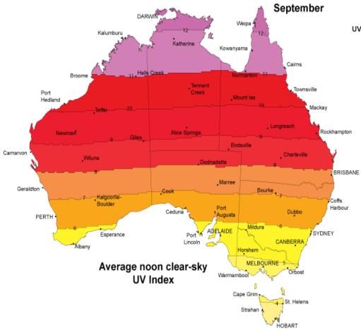
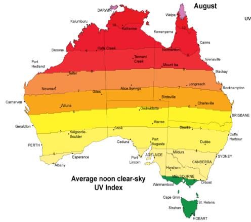
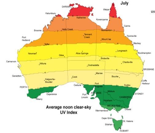
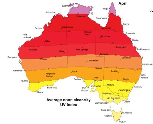
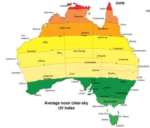
155 This study aims to apply a CLSTM hybrid machine learning model, which can exploit the

156 benefits of both convolutional layers (i.e., important feature extraction) and LSTM layers (i.e.,

157 storing sequence data for an extended period) and evaluate its ability to efficiently forecast the

158 UVI for the next day. The model was constructed and fed with hydro-climatic data in association

159 with UV irradiance in the Australian context. The model was optimized using ant colony

160 optimization, genetic algorithm, particle swarm optimization, and differential evolutional

161 algorithms. The model accuracy (i.e., efficiency and errors involved in UVI estimations) was

162 assessed with the conventional standalone data-driven models’ (e.g., SVR, decision tree, MLP,

163 CNN, LSTM, gated recurrent unit (GRU), etc.) performance statistics. The inference obtained

164 from the modeling results was also discussed that could be tremendously useful in building expert

165 judgment to protect public health in the Australian region and beyond.

166 2. Materials and Methods

167 2.1 Study area and UVI data

168 The study assessed the solar ultraviolet index of Perth (Latitude: -31.93oE and Longitude:

169 115.10oS), Western Australia. The Australian Radiation Protection and Nuclear Safety Agency

170 (ARPANSA) provided the UVI data of Australia (ARPANSA, 2021). Figure 1 shows the monthly

171 UVI data, the location of Perth, and the assessed station. The figure shows that Perth has low to

172 extreme UV concentration over the year between 1979 – 2007. The Summer season (December to

173 February) had the most extreme UV concentration, whereas the Autumn (March to May) has

174 moderate to high, and Winter (June to August) demonstrates lower to moderate, and Spring

175 (September to November) has higher to extreme UVI value in Perth.

176 Malignant melanoma rates in Western Australia are second only to those in Queensland,

177 Australia’s most populated state (Slevin et al., 2000). Australia has the highest incidence of NMSC

178 (Non-melanoma skin cancer) globally (Anderiesz et al., 2006; Staples et al., 1998). Approximately

179 three-quarters of the cancer cases have basal cell carcinoma (BCC) and squamous cell carcinoma

180 (SCC) types. These are attributed to the fair-skinned population’s high exposure to ambient solar

181 radiation (Boniol, 2016; McCarthy, 2004). As a result, Australia is seen as a world leader in public

182 health initiatives to prevent and detect skin cancer. Programs that have brought awareness of

183 prevention strategies and skin cancer diagnoses have data to show that people act on their

184 knowledge (Stanton et al., 2004). Many research showed that reducing sun security measures is

185 linked to reducing rates of BCC and SCC in younger groups. They might have received cancer

186 prevention messages as children (Staples et al., 2006). Considering the diversified concentration

187 of UVI concentration, this study considers Perth as an ideal study area.

188 2.2 Datasets of predictor variables

189 Three distinct data sources were used to collect the predictor variables in this analysis. The

190 Moderate Resolution Imaging Spectroradiometer (MODIS) satellite datasets are used to capturing

191 land surface status and flow parameters at regular temporal resolutions. These are supplemented

192 by ground-based Scientific Information for Landowners (SILO) repository meteorological data for

193 biophysical modeling and climate mode indices to help achieve Sea Surface Temperature (SST)

194 over Australia. Geospatial Online Interactive Visualization and Analysis Infrastructure

195 (GIOVANNI) is a geoscience data repository that provides a robust online visualization and

196 analysis platform for geoscience datasets. It collects data from over 2000 satellite variables (Chen

197 et al., 2010). The MODIS- aqua yielded 8 predictor variables for our study: a high-temporal

198 terrestrial modeling system consisting of a surface state and providing daily products with a high

199 resolution (250 m at nadir). A list of predictors of the MODIS Satellite can be obtained from the

200 National Aeronautics and Space Administration (NASA) database (Giovanni, 2021).

201 The surface UVI is influenced by atmospheric attenuation of incident solar radiation (Deo

202 et al., 2017). The angle subtended from the zenith (θs) to the solar disc is another factor that affects

203 the intensity of solar UV radiation (Allaart et al., 2004). The ultraviolet attenuation of clear-sky

204 solar radiation is dependent on ozone and atmospheric aerosol concentrations, along with cloud

205 cover (Deo et al., 2017). This implies that the measurements of biologically effective UV

206 wavelengths are affected by total column ozone concentration. Incident radiation at the Earth’s

207 surface is reduced by aerosols such as dust, smoke, and vehicle exhausts (Downs et al., 2016;

208 Román et al., 2013). Moreover, Lee et al. (2009) found a significant correlation between UV solar

209 radiation and geopotential height. Considering the direct influence of the predictors over ultraviolet

210 radiation and UV index, this study collected Ozone total column, aerosol optical depth (550nm

211 and 342.5nm), geopotential height, cloud fraction, and combined cloud optical thickness data from

212 the Geospatial Online Interactive Visualization and Analysis Infrastructure (GIOVANNI)

213 repository.

214 Therefore, meteorological predictor variables (i.e., temperature, u- and v-winds) were

215 significant while modeling UVI (Lee et al., 2009). Moreover, the cloud amount and diurnal

216 temperature range have a strong positive correlation, while rainfall and cloud amount show a

217 strong negative correlation (Jovanovic et al., 2011). Although overall cloud patterns agree with

218 rainfall patterns across Australia, the higher-quality cloud network is too coarse to represent

219 topographic influences accurately. Changes in the amount of cloud cover caused by climate change

220 can result in long-term changes in maximum and minimum temperature. Owing to the relations of

221 hydro-meteorological variables with UVI and their interconnections with cloud cover, the study

222 selected nine meteorological variables from the Scientific Knowledge for Land-Owners (SILO)

223 database to expand the pool of predictor variables, allowing for more practical application and

224 model efficiency. SILO data are managed by Queensland’s Department of Environment and

225 Research and can be obtained from https://www.longpaddock.qld.gov.au/silo.

226 Aerosol-rainfall relationships are also likely to be artifacts of cloud and cloud-clearing

227 procedures. During the Madden-Julian Oscillation (MJO) wet phase, the high cloud's value

228 increases, the cloud tops rise, and increased precipitation enhances wet deposition, which reduces

229 aerosol mass loading in the troposphere (Tian et al., 2008). The MJO (Lau and Waliser, 2011;

230 Madden and Julian, 1994, 1971) dominates the intra-seasonal variability in the tropical

231 atmosphere. A relatively slow-moving, large-scale oscillation in the deep tropical convection and

232 baroclinic winds exists in the warmer tropical waters in the Indian and western Pacific Oceans

233 (Hendon and Salby, 1994; Kiladis et al., 2001; Tian et al., 2008). The study used the Real-time

234 Multivariate MJO series 1 (RMM1) and 2 (RMM2) obtained from the Bureau of Meteorology,

235 Australia (BOM, 2020). Though RMM1 and RMM2 indicate an evolution of the MJO independent

236 of season, the coherent off-equatorial behavior is strongly seasonal (Wheeler and Hendon, 2004).

237 Pavlakis et al. (2008, 2007) studied the spatial and temporal variation of long surface wave and

238 short wave radiation. A high correlation was found between the longwave radiation anomaly and

239 the Niño3.4 index time series over the Niño3.4 region located in the central Pacific.

240 Moreover, Pinker et al. (2017) investigated the effect of El Niño and La Nina cycles on

241 surface radiative fluxes and the correlations between their anomalies and a variety of El Niño

242 indices. The maximum variance of anomalous incoming solar radiation is located just west of the

243 dateline. It coincides with anomalous SST (Sea surface temperature) gradient in the traditional

244 eastern Pacific El Niño Southern Oscillation (ENSO). However, we derive the Southern

245 Oscillation Index highly correlated with solar irradiance and mean Northern Hemisphere

246 temperature fluctuations reconstructions (Yan et al., 2011). In North America and the North

247 Pacific, land and sea surface temperatures, precipitation, and storm tracks are determined mainly

248 by atmospheric variability associated with the Pacific North American (PNA) pattern. The modern

249 instrumental record indicates a recent trend towards a positive PNA phase, which has resulted in

250 increased warming and snowpack loss in northwest North America (Liu et al., 2017). This study

251 used fifteen climate mode indices to increase the diversity.

252 2.3 Standalone models

253 2.3.1 Multiple layer perceptron (MLP)

254 The MLP is a simple feedforward neural network with three layers and is commonly used as a

255 reference model for comparison in machine learning application research (Ahmed and Lin, 2021).

256 The three layers are the input layer, a hidden layer with n-nodes, and the output layer. The input

257 data are fed into the input layer, transformed into the hidden layer via a non-linear activation

258 function (i.e., a logistic function). The target output is estimated, Eq. (1).

259 = (∑ + ) (1)

260 where = the vector of weights, = the vector of inputs, = the bias term; = the non-linear

 1
261 sigmoidal activation function, i.e., ( ) = .
 1+ − 

262 The computed output is then compared with the measured output, and the corresponding loss, i.e.,

263 the mean squared error (MSE), is estimated. The model parameters (i.e., initial weights and bias)

264 are updated using a backpropagation method until the minimum MSE is obtained. The model is

265 trained for several iterations and tested for new data sets for prediction accuracy.

266 2.3.2 Support vector regression (SVR)

267 The SVR is constructed based on the statistical learning theory. In SVR, a kernel trick is applied

268 that transfers the input features into the higher dimension to construct an optimal separating

269 hyperplane as follows (Ji et al., 2017):

270 ( ) = . ( ) + (2)

271 where w is the weight vector, b is the bias, and ( ) indicates the high-dimensional feature space.

272 The coefficients w and b, which define the location of the hyperplane, can be estimated by

273 minimizing the following regularized risk function:
 1
274 Minimize: || 2 || + ∑ 1( + ∗ ) (3)
 2

275 Subject to − . ( ) − ≤ + ; . ( ) + − ≤ + ∗ ; ≤ 0; ∗ ≤ 0

276 where C is the regularization parameter, and ∗ are slack variables. The Eq. (7) can be solved in

277 a dual form using the Lagrangian multipliers as follows:
 1
278 Maximize: − ∑ =1 ∑ =1( − ∗ ) ( − ∗ ) ( , ) − ∑ =1( − ∗ ) + ∑ = ∗
 1 ( − ) 
 2

279 (4)

280 Subject to ∑ =1( − ∗ ) = 0; , ∗ ∈ [0, ]

281 Where, ( , ) is the non-linear kernel function. In this present study, we used a radial basis

282 function (RBF) as the kernel, which is represented as follows:

 −|| − ||2
283 ( , ) = ( 2 2
 ), where is the bandwidth of the RBF.

284 2.3.3 Decision tree (DT)

285 A decision tree is a predictive model used for both classification and regression analysis (Jiménez-

286 Pérez and Mora-López, 2016). As our data is continuous, we used it for the regression predictions.

287 It is a simple tree-like structure that uses the input observations (i.e., x1, x2, x3, …, xn) to predict

288 the target output (i.e., Y). The tree contains many nodes, and at each node, a test to one of the

289 inputs (e.g., x1) is applied, and the outcome is estimated. The left/right sub-branch of the decision

290 tree is selected based on the estimated outcome. After a specific node, the prediction is made, and

291 the corresponding node is termed the leaf node. The prediction averages out all the training points

292 for the leaf node. The model is trained using all input variables and corresponding loss; the mean

293 squared error (MSE) is calculated to determine the best split of the data. The number of maximum

294 features is set as the total input features during the partition.

295 2.3.4 Convolutional neural network (CNN)

296 The CNN model was originally developed for document recognition (Lecun et al., 1998)

297 and used for predictions. Aside from the input and output layer, the CNN architecture has three

298 hidden layers: the convolutional layers, the pooling layers, and a fully connected layer. The

299 convolutional layers abstract the local information from the data matrix using a kernel. The

300 primary advantage of this layer is the implementation of weight sharing and spatial correlation

301 among neighbors (Guo et al., 2016). The pooling layers are the subsampling layers that reduce the

302 size of the data matrix. A fully connected layer is similar to the traditional neural network added

303 at the final pooling layer after completing an alternate stack of convolutional and pooling layers.

304 2.3.4 Long short-term memory (LSTM)

305 An LSTM network is a special form of recurrent neural network that stores sequence data

306 for an extended period (Hochreiter and Schmidhuber, 1997). The LSTM structure has three gates:

307 an input gate, an output gate, and a forget gate. The model regulates all these three gates and

308 determines how much data from previous time steps must be stored and transferred to the next

309 steps. The input gate controls the input data at the current time as follows:

310 = ∑ =1 + ∑ −1
 ℎ=1 ℎ ℎ + ∑ =1 −1 ; = ( ) (5)

311 Where = the input received from the ith node at time t; ℎ −1 = the result of the hth node at time

312 t-1; −1 = the cell state (i.e., memory) of the cth node at time t-1. The symbol ‘w’ represents the

313 weight between nodes, and the f is the activation function. The output gate transfers the current

314 value from Eq. (5) to the output node, Eq. (6). Then, at the final stage, the current value is stored

315 as the cell state in the forget gate, Eq. (7).

316 
 = ∑ =1 + ∑ −1
 ℎ=1 ℎ ℎ + ∑ =1 −1 ; 
 
 = ( ) (6)

317 ∅ = ∑ =1 ∅ + ∑ −1
 ℎ=1 ℎ∅ ℎ + ∑ =1 ∅ −1 ; ∅ = ( ∅ ) (7)

318 2.3.5 Gated recurrent unit (GRU) network

319 The GRU network is an LSTM variant having only two gates, such as reset and update gates (Dey

320 and Salem, 2017). The implementation of this network can be represented by the following

321 equations, Eq. (14-17):

322 = ( + ℎ −1 + ) (8)

323 = ( + ℎ −1 + ) (9)

324 = ∅( + (ℎ −1 . ) + ) (10)

325 ℎ = (1 − )ℎ −1 + . (11)

326 where = the sigmoidal activation function; = the input value at time t; ℎ −1 = the output value

327 at time t-1; and the , , , , , are the weight matrices for each gate and cell state.

328 The symbols r and z represent the reset and update gates, respectively. ∅ is the activation function,

329 and the dot [.] represents the element-wise dot product.

330 2.4 The proposed hybrid model

331 2.4.1 CLSTM (or CNN-LSTM) Hybrid Model

332 In this paper, a deep learning method using optimization techniques is constructed on top

333 of a forecast model framework. This study demonstrates how the CNN-LSTM (CLSTM) model,

334 comprised of four-layered CNN, can be effectively used for UVI forecasting. The CNN is

335 employed to integrate extracted features to forecast the target variable (i.e., UVI) with minimal

336 training and testing error. Likewise, the CNN-GRU (CGRU) hybrid model is prepared for the same

337 purpose.

338 2.5 Optimization techniques

339 2.5.1 Ant colony optimization
340 Ant colony optimization (ACO) algorithm model is the graphical representation of the real

341 ants’ behavior. In general, ants live in colonies, and they forage for food as a whole by

342 communicating with each other using a chemical substance, the pheromones (Mucherino et al.,

343 2015). An isolated ant cannot move randomly; they always optimize their way towards the food

344 deposit to their nests by interacting with previously laid pheromones marks on the way. The entire

345 colony optimizes their routes with this communication process and establishes the shortest path to

346 their nests from feeding sources (Silva et al., 2009). In ACO, the artificial ants find a solution by

347 moving on the problem graph. They deposit synthetic hormone pheromones on the graph so that

348 upcoming artificial ants can follow the pattern to build a better solution. The artificial ants calculate

349 the model's intrinsic mode functions (IMFs) anticipation by testing artificial pheromone values

350 against the target data. The probability of finding the best IMFs increases for every ant because of

351 changing pheromones value throughout the IMFs. The whole process is just like ant’s behavior of

352 finding the optimal option to reach the target. The probability ( ) of selecting the shortest

353 distance between the target and the IMFs of the input variable can be mathematically expressed as

354 follows (Prasad et al., 2019):

 ( +∆ ( ))2
355 ( ) = ( +∆ ( ))2 +( +∆ ( ))2
 (12)

356 Where ∈ {1,2} denotes decision point, and express as short and long distance to the target at

357 an instant is the total amount of pheromone ∆ ( ). The probability of the longest path can be

358 determined where ( ) + ( ) = 1. The testing update on the two branches is described as

359 follows:

360 ∆ ( ) = ∆ ( − 1) + ( − 1) ( − 1) + ( − 1) ( − 1) (13)

361 ∆ ( ) = ∆ ( − 1) + ( − 1) ( − 1) + ( − ) ( − ) (14)

362 Where , ∈ {1,2} and the value of represent the remainder in the model. ( ) denotes the

363 number of ants in the node at a certain period is given by:

364 ( ) = ( − 1) ( − 1) + ( − ) ( − ) (15)

365 The ACO algorithm is the most used simulation optimization algorithm where myriad artificial

366 ants work in a simulated mathematical space to search for optimal solutions for a given problem.

367 The ant colony algorithm is dominant in multi-objective optimization as it follows the natural

368 distribution and self-evolved simple process. However, with the increase of network information,

369 the ACO algorithm faces various constraints such as local optimization and feature redundancy

370 for selecting optimal pathways (Peng et al., 2018).

371 2.5.2 Differential evaluation optimization

372 The differential evolution (DEV) algorithm is renowned for its simplicity and powerful stochastic

373 direct search method. Besides, DEV has proven an efficient and effective method for searching

374 global optimal solutions for the multimodal objective function, utilizing N-D-dimensional

375 parameter vectors (Seme and Štumberger, 2011). It does not require a specific starting point, and

376 it operates effectively on a population candidate solution. The constant value N denotes the

377 population; in every module, a new generation solution is determined and compared with the

378 previous generation of the population member. It is a repetition process and runs until it reaches

379 the maximum number of generations (i.e., Gmax). The defines the generation number of

380 populations which can be written in mathematical proportional order. If the initial population

381 vector is , then = 1, , 2, … … , , , and = 0, … , 

382 , , = 1,2, … … . . , 

383 The initial population =0 is generated using random within given boundaries, which can be

384 written in the following equation:

 ( ) ( ) ( )
385 ,0 = [0,1]( − ) + , = 1,2, … , , = 1,2, … , (16)

386 Where [0,1] is the uniformly distributed number at the interval [0,1], which is chosen a new

387 for each . represents the boundary condition. In contrast, ( ) and ( ) represents the upper and

388 lower limit of the boundary vector parameters. For every generation, a new random vector is

389 randomly created, selecting vectors from the previous generation from the following manner:

 , −1 + ( , −1 − , −1 ) [0,1] ≤
390 , ={ } (17)
 , −1 ℎ 

391 Where, is the number of optimizations, is the candidate vector, ∈ [0,1] and ∈ [0,2]

392 control parameter. is the randomly selected index that ensures the difference between the

393 candidate vector and the generation vector. The population for new the new generation will be
 
394 assembled from the vector of the previous generation −1 and the candidate vectors , the

395 following equation can describe selection:

396 = 0, … , ; = 1,2, … … . . , 

 ( ) ≤ ( −1
 
 )
397 = { } (18)
 −1 ℎ 

398 The process repeats with the following generation population number until it satisfies the pre-

399 defined objective function.

400 2.5.3 Particle swarm optimization
401 The particle swarm optimization (PSO) method was developed for continuous non-linear

402 functions optimization having roots in artificial life and evolutionary computation (Kennedy and

403 Eberhart, 1995). The method was constructed using a simple concept that tracks each particle’s

404 current position in the swarm by implementing a velocity vector for particle’s previous to the new

405 position. However, the movement of the particles in the swarm depends on the individuals’

406 external behavior. Therefore, the process is very speculative, uses each particle's memory for

407 calculating new position, and gained knowledge by the swarm as a whole. Nearest neighbor

408 velocity matching and craziness, eliminating ancillary variables and incorporate multidimensional

409 search and acceleration by distance, were the precursor of PSO algorithm simulation (Eberhart and

410 Shi, 2001). Each particle in the simulation coordinates in the n-dimensional space calculation and

411 responds to the two quality factors called ‘gbest’ and ‘pbest’. gbest represents the best location

412 and value of particle in the population globally, and pbest represents the best-fitted solution

413 achieved by the particle so far in the population swarm. Thus, at each time step in the swarm, the

414 PSO concept stands, each particle changing its acceleration towards its two best quality factor

415 locations. The acceleration process begins by separating random numbers and presenting the

416 optimal ‘gbest’ and ‘pbest’ locations. The basic steps for the PSO algorithm are given below,

417 according to (Eberhart and Shi, 2001):

418 1. The process starts with initializing sample random particles with random velocities and

419 locations on n-dimensions in the design space.

420 2. The velocity vector for each particle in the swarm is carried out in the next step as the initial

421 velocity vector value.

422 3. Plot the velocity vector value and compare particle fitness evaluation with particle’s pbest.

423 If the new value is better than the initial value, update the new velocity vector value as

424 pbest and previous location equal to the current location in the design space.

425 4. In this step, compare the fitness evaluation with the particles’ overall previous global best.

426 If the current value is better than gbest, update it to a new gbest value and location.

427 5. The velocity and position of the particle can be changed according to the equations:

428 = + 1 ∗ ( ) ∗ ( − ) + 2 ∗ ( ) ∗ ( − ) (19)

429 = + (20)

430 6. Repeat step 2 and continue until the sufficiently fitted value and position are achieved.

431 Particle swarm optimization is well known for its simple operative steps and performance for

432 optimizing a wide range of functions. PSO algorithm can successfully solve the design problem

433 with many local minima and deal with regular and irregular design space problems locally and

434 globally. Although PSO can solve problems more accurately than other traditional gradient-based

435 optimizers, the computational cost is higher in PSO (Ventor and Sobieszczanski-Sobieski, 2003).

436 2.5.4 Genetic algorithm
437 The genetic algorithm (GA) is a heuristic search method based on natural selection and

438 evolution principles and concepts. This method was introduced by John Holland in the mid-

439 seventies, inspired by Darwin’s theory of descent with modification by natural selection. To

440 determine the optimal set of parameters GA mimics the reproduction behavior of the biological

441 populations in nature. It has been proven effective for the selection process in solving cutting-edge

442 optimization problems. It can also handle regular and irregular variables, non-traditional data

443 partitioning, and non-linear objective functions without requiring gradient information (Hassan et

444 al., 2004). The basic steps for the PSO algorithm are given below:

445 1. The determination of the maximum outcomes from an objective function, the genetic

446 algorithm uses the following function (Mayer and Lobet, 2018):

447 = (( 1 + 2 ), … . ( + +1 ) ) (21)

448 where is the number of decision variables ∈ [ , ] with a discretization step . The

449 initial boundary conditions , determined in the beginning of the simulation. is the

450 determines the physical parameters performances in the experiment. These decision variables

451 are represented by a sequence of binary digits ( ).

452 2. The decisions variables are given within initial boundary conditions = +

453 ( ) ∗ , where ∈ [0, 2 − 1] refers to the value of GENES. is the bit

454 length of each GENE, which is the first integer where +2 − 1 ∗ ≥ . The

455 total number of bits in each DNA refers = ∑ =1 . The algorithm process starts with

456 a random selection of objectives. After evaluation of each objective in the fitness function

457 = (( 1 + 2 ), … . ( + +1 ) ), and rank them from best to worst.

458 The genetic similarity determines the selection progress indicator. These random individual

459 objectives with rank are transferred to the next generation. The remaining individuals participate

460 in the steps of selection, crossover, and mutation. The individual objective parent selection process

461 can happen several times, and this can be achieved by many different schemes, such as the roulette-

462 wheel ranked method. For any pair of objective parents’ selection, crossover, and mutation process

463 of next-generation is defined. After that, the fitness of all individuals scheduled for the next

464 generation is evaluated. This process repeats from generation to generation until a termination

465 criterion is met.

466 GA methodology is quite similar to another stochastic searching algorithm PSO. Both

467 methods begin their search from a randomly generated population of designs that evolve over

468 successive generations. They do not require any specific starting point for the simulation. The first

469 operator is the “selection” procedure similar to “Survival for the Fittest” principle. The second

470 operator is the “Crossover” operator, which mimics mating in a biological population. Both

471 methods use the same convergence criteria for selecting the optimal solution in the problem space

472 (Hassan et al., 2004). However, GA differs in two ways from the most traditional optimization

473 methods. First, GA does not operate directly on the design parameter vector but a symbolic

474 parameter known as a chromosome. Second, it optimizes the whole design chromosomes at once,

475 unlike other optimization methods single chromosome at a time (Weile and Michielssen, 1997).

476 2.5.5 Complete Ensemble Empirical Mode Decomposition with Adaptive Noise (CEEMDAN)

477 The complete ensemble empirical mode decomposition with adaptive noise (CEEMDAN)

478 decomposition approach initiates by discretizing the n-length predictors of any model χ(t) into

479 IMFs (intrinsic model functions) and residues to conform with tolerability. However, to ensure no

480 information leakage in the IMFs and residues, the decomposition is performed separately by taking

481 training and testing subsets. The actual IMF is produced by taking the mean of the Empirical mode

482 decomposition (EMD)-grounded IMFs across a trial and combining white noise to model the

483 predictor-target variables. The CEEMDAN is used in machinery, electricity, and medicine such as

484 impact signal denoising, daily peak load forecasting, health degradation monitoring for rolling

485 bearings, friction signal denoising combined with mutual information (Li et al., 2019).

486 The CEEMDAN process is as follows:

487 Step 1: The decomposition of p-realizations of [ ] = 1 [ ] using EMD to develop their first

488 intrinsic approach, as explained according to the equation:

489 ̂1 [ ] = 1 ∑ =1 1 [ ] = 
 ̅ 1 [ ] (23)
 
490 Step 2: Putting k = 1, the 1st residue is computed following Eq. (1).

491 ̂1 [ ]
 1 [ ] = [ ] − (24)

492 Step 3: Putting k = 2, the 2nd residual is obtained as

493 ̂2 [ ] = 1 ∑ =1 1 ( 1 [ ] + 1 1 ( [ ]))
 (25)
 
494 Step 4: Setting k = 2… K calculates the kth residue as.

495 ̂ [ ]
 [ ] = −1 [ ] − (26)

496 Step 5: Now, we decompose the realizations [ ] + 1 1 ( [ ]), Here, = 1, … until

497 their first model of EMD is reached; Here the (k + 1) is

498 ̂( +1) [ ] = 1 ∑ =1 1 ( [ ] + ( [ ]))
 (27)
 

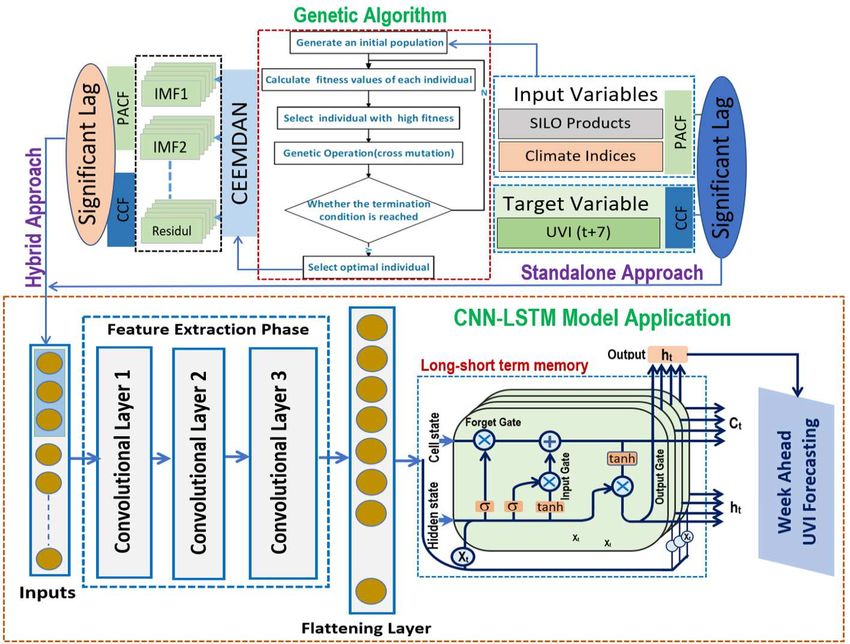
499 Step 6: Now, the k value is incremented, and steps 4–6 are repeated. Consequently, the final

500 residue is achieved:

501 [ ] = [ ] − ∑ ̂
 =1 (28)

502 Here, K is defined as the limiting case (i.e., the highest number of modes). To comply with the

503 replicability of the earliest input, [ ]., the following is performed for the CEEMDAN approach.

504 [ ] = ∑ ̂
 =1 + [ ] (29)

505

506 2.6 Model implementation procedure

507 It is crucial to optimize the objective model’s architecture to incorporate the relationship between

508 predictors and model. A multi-phase CNN-GRU and GRU model is included, built using Python-

509 based deep learning packages such as TensorFlow and Keras. A total of nine statistical metrics

510 was used to investigate the forecasting robustness of the models that have been integrated. The

511 model was powered by an Intel i7 @ 3.6GHz processor and 16 GB of memory. Deep learning

512 libraries like Keras (Brownlee, 2016; Ketkar, 2017) and TensorFlow (Abadi et al., 2016) were

513 used to demonstrating algorithms for the proposed models. In addition, packages like matplotlib

514 (Barrett et al., 2005) and seaborn (Waskom, 2021) were used for visualization.

515 The determination of the model’s valid predictors does not have any precise formula.

516 However, the literature suggests three methods, i.e., trial-and-error, the autocorrelation function

517 (ACF) and partial autocorrelation function (PACF), and the cross-correlation function (CCF)

518 approaches, for selecting lagged UVI memories and predictors to make an optimal model. In this

519 study, the PACF was used to determine significant antecedent behavior in terms of the lag of UVI

520 (Tiwari and Adamowski, 2013; Tiwari and Chatterjee, 2010). Figures 6b and 7b demonstrated the

521 PACF for UVI time series showing the antecedent behavior in terms of the lag of UVI and

522 decomposed UVI (i.e., IMFn) where antecedent daily delays are apparent. Generally, the CCF

523 selects the input signal pattern based on the predictors’ antecedent lag (Adamowski et al., 2012).

524 The CCF determined the predictors’ statistical similarity to the target variable (Figures 6a and 7a).

525 A set of significant input combinations was selected after evaluating each predictor’s rcross with

526 UVI. The figure shows that the highest correlation between p data and UVI was found for all

527 stations at lag zero (i.e., rcross = 0.22 – 0.75). AOD and GBI both demonstrated significant rcross

528 from 0.65 to 0.80 and 0.68 to 0.75, respectively. Some predictors with insignificant lags such as

529 AO, CT, and OTC were also considered to increase the predictors' diversity. The CCF with UVI

530 with predictors significantly varied for all other stations. However, selecting lags from the cross-

531 correlation function is identical to that used in the objective stations.

532 As mentioned, the CEEMDAN method was used to decompose the data sets. The daily

533 time series of UVI data and predictor variables were decomposed into respective daily IMFs and

534 a residual component using CEEMDAN procedures. The example of the IMFs and the residual

535 component of the respective CEEMDAN is shown in Figure 3. PACF was applied to the daily

536 IMFs and residual component time series generated in the above process. An individual input

537 matrix was created for each IMF, and the residual component was made up based on the significant

538 lagged memory with that of IMF of target UVI. These separate input matrices were used to forecast

539 the respective future IMFs and the residual component. Next, the anticipated IMFs and residuals

540 were combined to produce daily forecasts of UVI values. Note that the CEEMDAN

541 transformations are completely self-adaptive and data-dependent multi-resolution techniques. As

542 such, the number of IMFs and the residual component generated are contingent on the nature of

543 the data.

544 The predictor variables were used to forecast the UVI were normalized between 0 and 1 to

545 minimize the scaling effect of different variables as follows:

 − 
546 = (30)
 − 

547 In Eq. (30), is the respective predictors, is the minimum value for the predictors, is

548 the maximum value of the data and is the normalized value of the data. After normalizing

549 the predictor variables, the data sets were partitioned: 70% of the data sets were considered training

550 data, 15% were used for testing, and the remaining 15% of the data sets were considered validation

551 data. The LSTM model was followed by developing a hybrid LSTM model with 3-layered CNN

552 and 4-layered LSTM, as illustrated in Figure 2. Using the conventional models, the traditional

553 antecedent lagged matrix of the daily predictors’ variables was applied. The prior application of

554 the optimization algorithm was made before using CCF and PACF and before significant

555 predictors being removed from the model. Table 2 shows the selected predictors using four

556 optimization techniques in association with the UVI.

557 2.7 Model performance assessment

558 In this study, the effectiveness of the deep learning hybrid model was assessed using a variety of

559 performance evaluation criteria, e.g., Pearson’s Correlation Coefficient (r), root mean square error

560 (RMSE), Nash- Sutcliffe efficiency (NS) (Nash and Sutcliffe, 1970), and mean absolute error

561 (MAE). The relative RMSE (denoted as RRMSE) and relative MAE (denoted as RMAE) were used

562 to explore the geographic differences between the study stations.

563 The exactness of the relationship between predicted and observed values was used to

564 evaluate the effectiveness of a predictive model. When the error distribution in the tested data is

565 Gaussian, the root mean square error (RMSE) is a more appropriate measure of model performance

566 than the mean absolute error (MAE) (Chai and Draxler, 2014), but for an improved model

567 evaluation, Legates-McCabe’s (LM) Index are used as more sophisticated and compelling

568 measures (Legates and McCabe, 2013; Willmott et al., 2012). Mathematically, the metrics are as

569 follows:

570 i) Correlation coefficient (r):
 2
 ∑ ̅̅̅̅̅̅ ̅̅̅̅̅̅
 =1( − )( − )
571 = { 2
 } (31)
 √∑ ( − 
 ̅̅̅̅̅̅ )2 ∑ ̅̅̅̅̅̅
 =1 =1( − )

572 ii) Mean absolute error (MAE):
 1
573 MAE = ∑N
 i=1| for− obs | (32)
 N

574 iii) Root mean squared error (RMSE):

 1
575 RMSE = √ ∑N
 i=1(UVIfor − obs )
 2 (33)
 N

576 iv) Nash-Sutcliffe Efficiency (NS):

 ∑N
 i=1( )
 2
577 NSE = 1 − [1 − 2 ]) (34)
 ∑N ̅̅̅̅̅̅
 i=1( − )

578 v) Legates–McCabe’s Index (LM):

 ∑N | |
579 = 1 − [∑Ni=1|| for− ̅̅̅̅̅̅
 
 obs
 ||
 ] (35)
 i=1 obs− obs

580 vi) Relative Root Mean Squared Error (RRMSE, %):

 1
 √ ∑N
 i=1( for− obs )
 2
 
581 (%) = 1 100 (36)
 ∑ ( )
 =1

582 vii) Relative Mean Absolute Error (RMAE, %):

1 N
 ∑ | for − obs |
 N i=1
583 (%) = 1 100 (37)
 ∑ ( )
 =1

584 In Eq. (31–37), and for represents the observed and forecasted values for ith test

585 ̅̅̅̅̅ and 
 value; ̅̅̅̅̅ refer to their averages, accordingly, and N is defined as the number of

586 observations, while the CV stands for the coefficient of variation.

587 3. Results
588
589 This section describes results obtained from the proposed hybrid deep learning model (i.e.,

590 CEEMDAN-CLSTM) and other hybrid models (i.e., CEEMDAN-CGRU, CEEMDAN-LSTM,

591 CEEMDAN-GRU, CEEMDAN-DT, CGRU, and CLSTM), and the standalone LSTM, GRU, DT,

592 MLP, and SVR models. The evolutionary algorithms (i.e., ACO, DEV, GA, and PSO) were

593 incorporated to obtain the optimum features in model building. Seven statistical metrics from Eqs.

594 (31) to (37) were used to analyze the models in the testing dataset and visual plots to justify the

595 forecasted results’ justification.

596 3.1 The evaluation of hybrid and standalone models

597 The hybrid deep learning model (i.e., CEEMDAN-CLSTM) demonstrated high r and NS

598 values and low RMSE and MAE compared to their standalone models (Table 3). The best overall

599 performance was recorded using the CEEMDAN-CLSTM model with the Genetic Algorithm with

600 the highest correlation (i.e., r = 0.996), the highest data variance explained (i.e., NS = 0.997), and

601 the lowest errors (i.e., RMSE = 0.162 and MAE = 0.119). The performance was followed by the

602 same model with Partial Swarm Optimisation (i.e., r ≈ 0.996; NS ≈ 0.992; RMSE ≈ 0.216; MAE

603 ≈ 0.163) and Ant Colony Optimisation (i.e., r ≈ 0.996; NS ≈ 0.993; RMSE ≈ 0.220; MAE ≈ 0.165).

604 The single deep learning models (i.e., LSTM and GRU) performed better than the single machine

605 learning models (i.e., DT, SVR, and MLP). Moreover, the hybrid deep learning models without a

606 CNN (i.e., CEEMDAN-GRU and CEEMDAN-GRU) also demonstrated higher forecasting

607 accuracy (i.e., r = 0.973 – 0.993; RMSE = 0.387 – 0.796) in comparison with standalone deep

608 learning models ( i.e., r ≈ 0.959 – 0.981; RMSE ≈ 0.690 – 0.986). The following models’

609 performance is then predicted by the CNN-GRU, CEEMDAN-GRU, and GRU models in that

610 order.

611 3.2 The selection of the best model

612 RRMSE and LM for all tested models were used to assess the robustness of the proposed

613 hybrid models as well as for comparisons. The magnitude of RRMSE (%) and LM for the objective

614 model (CEEMDAN-CLSTM) shown in Figure 6 indicates that the proposed hybrid model

615 performed significantly better than other benchmark models. The RRMSE and LM values ranged

616 between 2 and 3.5 percent and between 0.982 and 0.991, respectively. The performance indices

617 (i.e., RRMSE and LM) using four optimization algorithms were higher for the CEEMDAN-CGRU

618 model. Overall, the CEEMDAN-CLSTM model with the GA optimization methods provided the

619 best performance (i.e., RRMSE = ~2.0%; LM = 0.991), indicating its high efficiency in forecasting

620 the future UV-Index a higher degree of accuracy.

621 A precise comparison of forecasted and observed UVI can also be seen by examining the

622 scatterplot of forecasted (UVIfor) and observed (UVIobs) UVI for four optimization algorithms (i.e.,

623 ACO, PSO, DEV, and GA) (Figure 7). Here, scatter plots showed the coefficient of determination

624 (r2) and a least-square fitting line, along with the equation for UVI and an observed UVI close to

625 the forecasted UVI. As demonstrated in Figure 7, it also appears that the proposed hybrid model

626 performed better when compared with other applied models. However, among the four