Extending a land-surface model with Sphagnum moss to simulate responses of a northern temperate bog to whole ecosystem warming and elevated CO2 ...
←
→
Page content transcription
If your browser does not render page correctly, please read the page content below
Biogeosciences, 18, 467–486, 2021
https://doi.org/10.5194/bg-18-467-2021
© Author(s) 2021. This work is distributed under
the Creative Commons Attribution 4.0 License.

Extending a land-surface model with Sphagnum moss to simulate
responses of a northern temperate bog to whole ecosystem
warming and elevated CO2
Xiaoying Shi1 , Daniel M. Ricciuto1 , Peter E. Thornton1 , Xiaofeng Xu2 , Fengming Yuan1 , Richard J. Norby1 ,
Anthony P. Walker1 , Jeffrey M. Warren1 , Jiafu Mao1 , Paul J. Hanson1 , Lin Meng3 , David Weston1 , and
Natalie A. Griffiths1
1 Climate Change Science Institute and Environmental Sciences Division, Oak Ridge National Laboratory,
Oak Ridge, TN, 37831, USA
2 Biology Department, San Diego State University, San Diego, CA, 92182-4614, USA
3 Department of Geological and Atmospheric Sciences, Iowa State University, Ames, IA, 50011, USA

Correspondence: Xiaoying Shi (shix@ornl.gov)

Received: 11 March 2020 – Discussion started: 6 May 2020
Revised: 20 November 2020 – Accepted: 23 November 2020 – Published: 20 January 2021

Abstract. Mosses need to be incorporated into Earth sys-        tion for the peatland ecosystem. Microtopography is critical:
tem models to better simulate peatland functional dynam-        Sphagnum mosses on hummocks and hollows were simu-
ics under the changing environment. Sphagnum mosses are         lated to show opposite warming responses (NPP decreasing
strong determinants of nutrient, carbon, and water cycling in   with warming on hummocks but increasing in hollows), and
peatland ecosystems. However, most land-surface models do       hummock Sphagnum was modeled to have a strong depen-
not include Sphagnum or other mosses as represented plant       dence on water table height. The inclusion of this new moss
functional types (PFTs), thereby limiting predictive assess-    PFT in global ELM simulations may provide a useful foun-
ment of peatland responses to environmental change. In this     dation for the investigation of northern peatland carbon ex-
study, we introduce a moss PFT into the land model com-         change, enhancing the predictive capacity of carbon dynam-
ponent (ELM) of the Energy Exascale Earth System Model          ics across the regional and global scales.
(E3SM) by developing water content dynamics and nonva-
scular photosynthetic processes for moss. The model was
parameterized and independently evaluated against obser-
vations from an ombrotrophic forested bog as part of the        Copyright statement. This paper has been authored by UT-Battelle,
Spruce and Peatland Responses Under Changing Environ-           LLC, under contract no. DE-AC05-00OR22725 with the US De-
                                                                partment of Energy. The publisher, by accepting the article for pub-
ments (SPRUCE) project. The inclusion of a Sphagnum PFT
                                                                lication, acknowledges that the United States government retains a
with some Sphagnum-specific processes in ELM allows it to       nonexclusive, paid-up, irrevocable, worldwide license to publish or
capture the observed seasonal dynamics of Sphagnum gross        reproduce the published form of this paper or allow others to do
primary production (GPP) albeit with an underestimate of        so for United States government purposes. The Department of En-
peak GPP. The model simulated a reasonable annual net           ergy will provide public access to these results of federally spon-
primary production (NPP) for moss but with less interan-        sored research in accordance with the DOE Public Access Plan
nual variation than observed, and it reproduced aboveground     (http://energy.gov/downloads/doe-public-access-plan).
biomass for tree PFTs and stem biomass for shrubs. Differ-
ent species showed highly variable warming responses un-
der both ambient and elevated atmospheric CO2 concentra-
tions, and elevated CO2 altered the warming response direc-

Published by Copernicus Publications on behalf of the European Geosciences Union.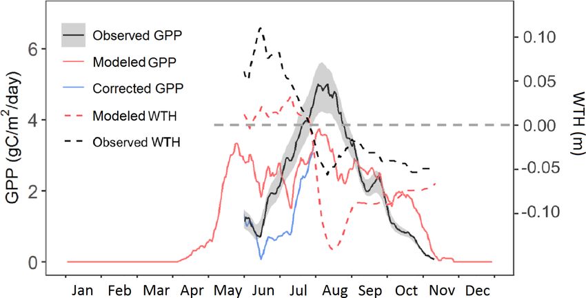
468                                     X. Shi et al.: Modeling the responses of Sphagnum moss to environmental changes

1   Introduction                                                  2009; Frolking et al., 2010). Several peatland-specific mod-
                                                                  els contain moss species and have been applied globally or
Boreal peatlands store at least 500 pg of soil carbon due         at selected peatland sites. For example, the McGill Wetland
to the incomplete decomposition of plant litter inputs re-        Model (MWM) was evaluated using the measurements at
sulting from a combination of low temperature and water-          Degerö Stormyr and the Mer Bleue bogs (St-Hilaire et al.,
saturated soils. Because of this capacity to store carbon, bo-    2010). The peatland version of the General Ecosystem Sim-
real peatlands have played a critical role in regulating the      ulator – Model of Raw Humus, Moder, and Mull (GUESS-
global climate since the onset of the Holocene (Frolking and      ROMUL) was used to simulate the changes in daily CO2 ex-
Roulet, 2007; Yu et al., 2010). The total carbon stock is large   change rates with water table position at a fen (Yurova et al.,
but uncertain: a new estimation of northern peatland carbon       2007). The PEATBOG model was implemented to character-
stock of 1055 pg was recently reported by Nichols and Pe-         ize peatland carbon and nitrogen cycles in the Mer Bleue bog,
teet (2019). The rapidly changing climate at high latitudes       including moss PFTs but without accounting for microtopog-
is likely to impact both primary production and decomposi-        raphy (Wu and Blodau, 2013). The CLASS-CTEM model
tion rates in peatlands, contributing to uncertainty in whether   (the coupled Canadian Land Surface Scheme and the Cana-
peatlands will continue their function as net carbon sinks in     dian Terrestrial Ecosystem Model), which includes a moss
the long term (Moore et al., 1998; Turetsky et al., 2002; Wu      layer as the first soil layer, was applied to simulate water, en-
and Roulet, 2014). Manipulative experiments and process-          ergy, and carbon fluxes at eight different peatland sites (Wu et
based models are thus needed to make defensible projections       al., 2016). The IAP-RAS (Institute of Applied Physics, Rus-
of the net carbon balance of northern peatlands under antici-     sian Academy of Sciences) wetland methane (CH4 ) model
pated global warming (Hanson et al., 2017; Shi et al., 2015).     with a 10 cm thick moss layer (Mokhov et al., 2007) was run
   Peatlands are characterized by a ground layer of               globally to simulate the distribution of CH4 fluxes (Wania
bryophytes, and the raised or ombrotrophic bogs of the bo-        et al., 2013). The CHANGE model (a coupled hydrologi-
real zone are generally dominated by Sphagnum mosses that         cal and biogeochemical process simulator), which includes
contribute significantly to total ecosystem CO2 flux (Oechel      a moss cover layer (Launiainen et al., 2015), was used to in-
and Van Cleve, 1986; Williams and Flanagan, 1998; Robroek         vestigate the effect of moss on soil temperature and carbon
et al., 2009; Vitt, 2014). Sphagnum mosses also strongly af-      flux at a tundra site in northeastern Siberia (Park et al., 2018).
fect the hydrological and hydrochemical conditions at the         Chadburn et al. (2015) added a surface layer of moss to the
raised bog surface (Van, 1995; Van der Schaaf, 2002). As          JULES land-surface model to consider the insulating effects
a result, microclimate and Sphagnum species interactions in-      and treated the thermal conductivity of moss depending on its
fluence the variability of both carbon accumulation rates and     water content to investigate the permafrost dynamics. Porada
water and exchanges within peatland and between peatland          et al. (2016) integrated a stand-alone dynamic nonvascular
and atmosphere (Heijmans et al., 2004a, b; Rosenzweig et          vegetation model LiBry (Porada et al., 2013) to land-surface
al., 2008; Brown et al., 2010; Petrone et al., 2011; Goetz        scheme JSBACH, but JSBACH mainly represents bryophyte
and Price, 2015). Functioning as a keystone species of bo-        and lichen cover in upland forest and not a peatland ecosys-
real peatlands, Sphagnum mosses strongly influence the nu-        tem. Druel et al. (2017) investigated the vegetation–climate
trient, carbon, and water cycles of peatland ecosystems (Nils-    feedbacks at high latitudes by introducing a nonvascular
son and Wardle, 2005; Cornelissen et al., 2007; Lindo and         plant type representing mosses and lichens to the global land-
Gonzalez, 2010; Turetsky et al., 2010, 2012) and exert a sub-     surface model ORCHIDEE. Moreover, those models did not
stantial impact on ecosystem net carbon balance (Clymo and        consider microtopography and the lateral transports between
Hayward; 1982; Gorham, 1991; Wieder, 2006; Weston et el.,         hummocks and hollows. Two models, the “ecosys” model
2015; Walker et al., 2017; Griffiths et al., 2018).               (Grant et al., 2012) and CLM_SPRUCE (Shi et al., 2015),
   Numerical models are useful tools to identify knowl-           have been parameterized to represent peatland microtopo-
edge gaps, examine long-term dynamics, and predict future         graphic variability (e.g., the hummock and hollow micro-
changes. Earth system models (ESMs) simulate global pro-          terrain characteristic of raised bogs) with lateral connections
cesses, including the carbon cycle, and are primarily used        across the topography. The prediction of water table dynam-
to make future climate projections. Poor model representa-        ics in the “ecosys” model is constrained by specifying a re-
tion of carbon processes in peatlands is identified as a defi-    gional water table at a fixed height and a fixed distance from
ciency, causing biases in simulated soil organic mass and het-    the site of interest, thereby missing key controlling factors of
erotrophic respiratory fluxes for current ESMs (Todd-Brown        a precipitation-driven dynamic water table (Shi et al., 2015).
et al., 2013; Tian et al., 2015). Although most ESMs do           The CLM_SPRUCE model (Shi et al., 2015) was developed
not include moss, a number of offline dynamic vegetation          to parameterize the hydrological dynamics of lateral trans-
models and ecosystem models do include one or more moss           port for microtopography of hummocks and hollows in the
plant functional types (PFTs) (Pastor et al., 2002; Nungesser,    raised bog environment of the SPRUCE (Spruce and Peat-
2003; Zhuang et al., 2006; Bond-Lamberty et al., 2007; Hei-       land Responses Under Changing Environments) experiment
jmans et al., 2008; Euskirchen et al., 2009; Wania et al.,        (Hanson et al., 2017). That model version did not include

Biogeosciences, 18, 467–486, 2021                                                      https://doi.org/10.5194/bg-18-467-2021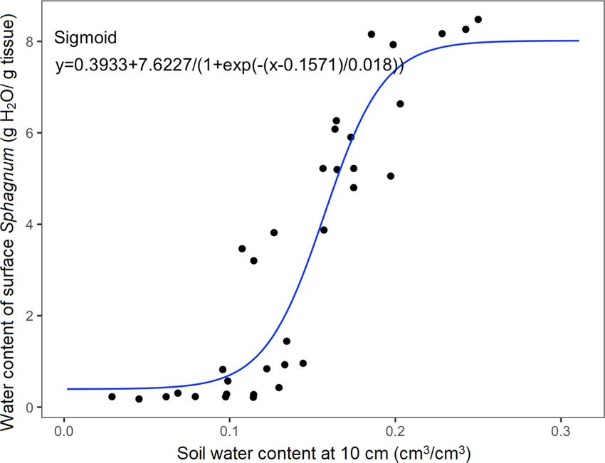
X. Shi et al.: Modeling the responses of Sphagnum moss to environmental changes                                                      469

the biophysical dynamics of Sphagnum moss, and it used a           Table 1. Physiological parameters of Sphagnum mosses as given in
prescribed leaf area instead of allowing leaf area to evolve       Hobbie (1996).
prognostically.
   In this study, we introduce a new Sphagnum moss PFT                   Parameters   Description                           Values
into the model and migrate the entire raised-bog capability              lflitcn      Leaf litter C : N ratio (g C / g N)      66
into the new Energy Exascale Earth System Model (E3SM),                  lf_fcel      Leaf litter fraction of cellulose     0.737
specifically into version 1 of the E3SM land model (ELM v1;              lf_flab      Leaf litter fraction of labile        0.227
Ricciuto et al., 2018). The objectives of this study are as fol-         lf_flig      Leaf litter fraction of lignin        0.036
lows: (1) to introduce a Sphagnum PFT to the ELM model
with additional Sphagnum-specific processes to better cap-
ture the peatland ecosystem and (2) to apply the updated           ported by Tables 1–3. We use the same framework as for
ELM to explore how an ombrotrophic, raised-dome bog peat-          C3 arctic grasses, but the Ball–Berry slope term is assumed
land ecosystem will respond to different scenarios of warm-        to be zero, and the intercept term is the conductance term
ing and elevated atmospheric CO2 concentration.                    as a function of water content of Sphagnum mosses. For
                                                                   all other processes like the evapo(transpi)ration and associ-
2     Model description                                            ated parameters not described below, we used the C3 arctic
                                                                   grasses equations reported by Oleson et al. (2013). Drying
2.1    Model provenance                                            impacts the conductance and affects evapo(transpi)ration of
                                                                   the internal water. The specific leaf area (SLA) and leaf C : N
ELM v1 is the land component of E3SM v1, which is sup-             ratio parameters are strong controls on the maximum rate of
ported by the US Department of Energy (DOE). Developed             Rubisco carboxylase activity (Vcmax) and therefore overall
by multiple DOE laboratories, E3SM consists of atmosphere,         productivity and Sphagnum moss leaf area index (LAI). The
land, ocean, sea ice, and land ice components linked through       high sensitivities occur because LAI is a strong control on
a coupler that facilitates across-component communication          evapo(transpi)ration.
(Golaz et al., 2019). ELM was originally branched from the
Community Land Model (CLM4.5; Oleson et al., 2013) with            2.3     New model developments
new developments that include representation of coupled car-
bon, nitrogen, and phosphorus controls on soil and vege-           2.3.1    Water content dynamics of Sphagnum mosses
tation processes and new plant carbon and nutrient storage
pools (Ricciuto et al., 2018; Yang et al., 2019; Burrows et        The main sources for water content of Sphagnum mosses are
al., 2020). Inputs of new mineral nitrogen of ELM are from         passive capillary water uptake from peat and the intercep-
atmospheric deposition and biological nitrogen fixation. The       tion of atmospheric water on the capitulum (growing tip of
fixation of new reactive nitrogen from atmospheric N2 by soil      the moss) (Robroek et al., 2007). Capillary water uptake, the
microorganisms is an important component of nitrogen bud-          internal Sphagnum moss water content, is modeled as func-
gets. ELM follows the approach of Cleveland et al. (1999)          tions of soil water content and evaporation losses. Water in-
that uses an empirical relationship of biological nitrogen fix-    tercepted on the Sphagnum moss capitulum is modeled as a
ation as a function of net primary production to predict the       function of moss foliar biomass, current canopy water, water
nitrogen fixation. The model version used in this study is des-    drip, and evaporation losses.
ignated ELM_SPRUCE and includes the new implementa-                   Since evaporation at the Sphagnum surface depends on the
tion of Sphagnum mosses, as well as the hydrological dy-           atmospheric water vapor deficit, moss–atmosphere conduc-
namics of lateral transport between hummock and hollow             tance, and available water pool which depends on capillary
microtopographies. The implementation has been parameter-          wicking of water up to the surface, we developed a relation-
ized based on observations from the S1-Bog in northern Min-        ship between measured soil water content at depth and sur-
nesota, USA, as described by Shi et al. (2015) with additional     face Sphagnum water content. At SPRUCE, the peat volu-
details provided below.                                            metric water content is measured at several depths using au-
                                                                   tomated sensors (model 10HS, Decagon Devices, Inc., Pull-
2.2    Nonvascular plants: Sphagnum mosses                         man, WA) calibrated for the site-specific upper peat soil us-
                                                                   ing mesocosms (reference Fig. S1 in the Supplement; Han-
To represent the nonvascular plant, Sphagnum mosses, we            son et al., 2017). During those calibrations, we periodically
modified the C3 arctic grasses equations as follows. We con-       sampled the surface Sphagnum for gravimetric water content
sidered Sphagnum biomass to be represented mainly by leaf          and water potential using a dew point potentiometer (WP4,
and stem carbon (only a very shallow root). In addition, we        Decagon Devices, Inc.) which also provided a surface soil
modified the vascular C3 arctic grasses equations for pho-         water retention curve. The destructive sampling of surface
tosynthesis and stomatal conductance (see below the new            Sphagnum was primarily hummock species but did include
model development) and the associated parameters as re-            some hollow species. The automated measurements of peat

https://doi.org/10.5194/bg-18-467-2021                                                        Biogeosciences, 18, 467–486, 2021
470 X. Shi et al.: Modeling the responses of Sphagnum moss to environmental changes
Table 2. PFT-specific optimized model parameters.
Parameter Description Sphagnum Picea Larix Shrub Range
flnr Rubisco-N fraction of leaf N 0.2906 0.0678 0.2349 0.2123 (0.05, 0.30)
croot_stem Coarse root to stem allocation ratio N/A 0.2540 0.1529 0.7540 (0.05, 0.8)
stem_leaf1 Stem to leaf allocation ratio N/A 1.047 1.016 0.754 (0.3, 2.2)
leaf_long Leaf longevity (yr) 0.9744 53 N/A N/A (0.75, 2.0)
slatop Specific leaf area at canopy top (m2 g C−1 ) 0.00781 0.00462 0.0128 0.0126 (0.004, 0.04)
leafcn Leaf C to N ratio 35.56 70.17 64.84 33.14 (20, 75)
froot_leaf2 Fine root to leaf allocation ratio 0.3944 0.8567 0.3211 0.6862 (0.15, 2.0)
mp Ball–Berry stomatal conductance slope N/A 7.50 9.32 10.8 (4.5, 12)
Optimized values of PFT-specific parameters. The range column values in brackets indicate the range of acceptable parameter values used in the sensitivity
analysis and the optimization across all four PFTs in the format (minimum, maximum). N/A indicates that parameter is not relevant for that PFT.
1 For tree PFTs, this parameter depends on NPP. The value shown is the allocation at an NPP of 800 g C m−2 yr−1 . 2 The fine root pool is used as a surrogate
for non-photosynthetic tissue in Sphagnum. 3 This parameter was not optimized; we used the default value.
Table 3. Non-PFT-specific optimized model parameters.
Description Optimized value Default Range
r_mort Vegetation mortality 0.0497 0.02 (0.005, 0.1)
decomp_depth_efolding Depth-dependence e-folding 0.3899 0.5 (0.2, 0.7)
depth for decomposition (m)
qdrai,0 Maximum subsurface drainage 3.896 ×10⁻⁶ 9.2 ×10−6 ∗ (0, 1 ×10⁻³ )
rate (kg m−2 s−1 )
Q10 _mr Temperature sensitivity of 2.212 1.5 (1.2, 3.0)
maintenance respiration
br_mr Base rate for maintenance 4.110 ×10⁻⁶ 2.52 ×10⁻⁶ (1 ×10⁻⁶ , 5 ×10⁻⁶ )
respiration (g C (g N)−1 s−1 )
crit_onset_gdd Critical growing degree days 99.43 200 (20, 500)
for leaf onset
lw_top_ann Live wood turnover proportion 0.3517 0.7 (0.2, 0.85)
(yr−1 )
gr_perc Growth respiration fraction 0.1652 0.3 (0.12, 0.4)
rdrai,0 Coefficient for surface water 6.978 ×10⁻⁷ 8.4 ×10−8 ∗ (1 ×10−9 , 1 ×10⁻⁶ )
runoff (kg m−4 s−1 )
Optimized and default values for non-PFT-specific parameters. The range column values in brackets indicate the range of acceptable parameter values used
in the sensitivity analysis and the optimization in the format (minimum, maximum).
∗ Previously calibrated value from Shi et al. (2015).
water content at 10 cm depth were shown to be a good indi- The Sphagnum moss surface water (Wsurface ) was calcu-
cator of surface Sphagnum water content (Fig. 1). Based on lated using the model predicted canopy water and the dry
this relationship, we model the water content of Sphagnum foliar biomass as follows:
moss due to capillary rise (Winternal ) (g water / g dry moss)
as follows: Wsurface = can_water/fmass, (2)
Winternal = 0.3933 + 7.6227/ (1 + exp (− (Soilvol where Wsurface (g water / g dry moss) is the surface water
−0.1571)) /0.018) , (1) content and fmass is the foliar biomass of Sphagnum mosses.
The can_water is the Sphagnum moss canopy water, and it is
where Soilvol is the averaged volumetric soil water of mod- simulated by a function of interception, canopy drip, dew,
eled soil layers nearest the 10 cm depth horizon (layers three and canopy evaporation (Oleson et al., 2013).
and four in the ELM v1 vertical layering scheme).
Biogeosciences, 18, 467–486, 2021 https://doi.org/10.5194/bg-18-467-2021X. Shi et al.: Modeling the responses of Sphagnum moss to environmental changes 471
sure (Ci ) of vascular PFTs:
1.4gs + 1.6gb
Ci = Ca − Patm An , (4)
gs gb
where Ci is the internal leaf CO2 partial pressure, Ca is the
atmospheric CO2 partial pressure, An is leaf net photosyn-
thesis (µmol CO2 m−2 s−1 ), Patm is the atmospheric pressure,
and values 1.4 and 1.6 are the ratios of the diffusivity of CO2
to H2 O for stomatal conductance and the leaf boundary layer
conductance, respectively.
For Sphagnum moss photosynthesis, we followed the
method from the McGill Wetland Model (St-Hilaire et al.,
2010; Wu et al., 2013), which is based on the effects of
Sphagnum moss water content on photosynthetic capac-
ity (Tenhunen et al., 1976) and total conductance of CO2
(Williams and Flanagan, 1998) and replaces the stomatal
Figure 1. The measured relationship between soil water content at conductance representation used for vascular PFTs.
depth and the water content of surface Sphagnum based on destruc- Patm An
tive sampling. Ci = Ca − . (5)
gtc
The total conductance to CO2 (gtc ) was determined from a
The total water content (Wtotal ) of Sphagnum mosses is least-squares regression described by Williams and Flana-
the sum of water taken up from peat and the surface water gan (1998) as follows:
content (St-Hilaire et al., 2010; Wu et al., 2013). 2
gtc = −0.195 + 0.134Wtotal − 0.0256Wtotal
3 4
Wtotal = Winternal + Wsurface . (3) + 0.0028Wtotal − 0.0000984Wtotal
5
+ 0.00000168Wtotal , (6)
2.3.2 Modeling Sphagnum CO2 conductance and where Wtotal is as defined in Eq. (3). This relationship is only
photosynthesis valid up to the maximum water holding capacity of mosses.
Note that we assume that the boundary layer conductance
ELM_SPRUCE computes photosynthetic carbon uptake is greater than moss surface layer conductance, and the moss
(gross primary production or GPP) for each vascular PFT on surface layer conductance is greater than chloroplast conduc-
a half-hourly time step based on the Farquhar biochemical tance.
approach (Farquhar et al., 1980; Collatz et al., 1991, 1992) In addition to the water content, the effects of moss sub-
with implementation as described by Oleson et al. (2013). mergence were taken into account in the calculation of moss
While Sphagnum lacks a leaf cuticle and stomata that regu- photosynthesis. Walker et al. (2017) reported significant im-
late water loss and CO2 uptake in vascular plants (Titus et al., pacts of submergence on measured Sphagnum GPP and mod-
1983), the primary transport pathway for CO2 is through the eled the effect by modifying the Sphagnum leaf (stem) area
cells and is analogous to mesophyll conductance in higher index. Submergence in Walker et al. (2017) was expressed as
plants. Thus, we calculate the total conductance to CO2 for photosynthesizing stem area index (SAI) as a logistic func-
Sphagnum mosses by using total water content following the tion of water table depth. A maximum SAI of 3 was used,
method reported by Williams and Flanagan (1998) described and the parameter combination that most closely described
below. Goetz and Price (2015) also indicated that capillary the GPP data gave a range of water table depth from −10 cm
rise through the peat is essential to maintain a water con- for complete submergence and SAI of ∼ 2.5 at 10 cm. This
tent sufficient for photosynthesis for Sphagnum moss species allowed for a range of processes such as floatation of Sphag-
but that atmospheric inputs can provide small but critical num with the water table and adhesion of water to the Sphag-
amounts of water for physiological processes. num capitula. For simplicity, in ELM_SPRUCE, we calcu-
The stomatal conductance for vascular plant types in lated such impacts on Sphagnum GPP directly as a function
ELM_SPRUCE is derived from the Ball–Berry conductance of the height of simulated surface water, assuming that GPP
model (Collatz et al., 1991). That model relates stomatal con- from the submerged portion of photosynthetic tissue is negli-
ductance to net leaf photosynthesis scaled by the relative hu- gible. GPP is thus reduced linearly according to the following
midity and the CO2 concentration at the leaf surface. The equation:
stomatal conductance (gs ) and boundary layer conductance
(gb ) are required to obtain the internal leaf CO2 partial pres- GPPsub = GPPorig × (hmoss − H2 Osfc ) , (7)
https://doi.org/10.5194/bg-18-467-2021 Biogeosciences, 18, 467–486, 2021472 X. Shi et al.: Modeling the responses of Sphagnum moss to environmental changes
where GPPsub is the GPP corrected for submergence ef- pretreatment net primary productivity (NPP) (Norby et al.,
fects, GPPorig is the original GPP, H2 Osfc is the surface wa- 2019). ELM_SPRUCE was driven by climate data (temper-
ter height, and hmoss is the height of the photosynthesizing ature, precipitation, relative humidity, solar radiation, wind
Sphagnum layer above the soil surface, set to 5 cm in our speed, pressure, and long-wave radiation) from 2011 to 2017
simulations. If H2 Osfc is equal to or greater than hmoss , GPP measured at the SPRUCE S1-Bog (Hanson et al., 2015a, b).
is reduced to zero. Because in our simulations surface water The surface weather station is outside of the enclosures and
is never predicted to occur in the hummocks, in practice this not impacted by the experimental warming treatments that
submergence effect only affects the moss GPP in the hollows. began in 2015. These data are available at https://mnspruce.
ornl.gov/ (last access: 13 January 2021).
3 Methods 3.3 Simulation of the SPRUCE experiment
3.1 Site description
Based on measurements at the SPRUCE site, ELM_SPRUCE
We focused on a high C, ombrotrophic peatland (the S1- includes four PFTs: boreal evergreen needleleaf tree (Picea),
Bog) that has a perched water table with limited groundwater boreal deciduous needleleaf tree (Larix), boreal deciduous
influence (Sebestyen et al., 2011; Griffiths and Sebestyen, shrub (representing several shrub species), and the newly in-
2016). This southern boreal bog is located in the Marcell troduced Sphagnum moss PFT. Currently, ELM_SPRUCE
Experimental Forest approximately 40 km north of Grand does not include light competition among multiple PFTs
Rapids, Minnesota, USA (lat 47.50283◦ , long −93.48283◦ ) and thus does not represent cross-PFT shading effects. Our
(Sebestyen et al., 2011), and is the site of the SPRUCE cli- model also allows the canopy density of PFTs to change
mate change experiment (http://mnspruce.ornl.gov, last ac- prognostically, and their fractional coverage is held constant.
cess: 13 January 2021; Hanson et al., 2017). The S1-Bog We used measurements from Sphagnum moss collected at
has a raised hummock and sunken hollow microtopography, a tussock tundra site in Alaska (Hobbie, 1996) to set sev-
and it is nearly covered by Sphagnum mosses. S. angusti- eral of the model leaf litter parameters for our simulations
folium (C.E.O. Jensen ex Russow) and S. fallax (Klinggr.) (Table 1). The values for other parameters have been opti-
occupy 68 % of the moss layer and exist in both hummocks mized based on observations at the SPRUCE site (Tables 2
and hollows. S. magellenicum (Brid.) occupies ∼ 20 % of and 3; optimization methods described in Sect. 3.4). We pre-
the moss layer and is primarily limited to the hummocks scribe both hummock and hollow microtopographies to have
(Norby et al., 2019). The vascular plant community at the the same fractional PFT distribution. Consistent with Shi et
S1-Bog is dominated by the evergreen tree Picea mari- al. (2015), hummocks and hollows were modeled on sepa-
ana (Mill.) B.S.P., the deciduous tree Larix laricina (Du rate columns with lateral flow of water between them. All the
Roi) K. Koch, and a variety of ericaceous shrubs. Trees are ELM_SPRUCE simulations were conducted using a prog-
present due to natural regeneration following strip cut har- nostic scheme for canopy phenology (Oleson et al., 2013).
vesting in 1969 and 1974 (Sebestyen et al., 2011). The soil of The SPRUCE experiment at the S1-Bog consists of com-
this peat bog is the Greenwood series, a Typic Haplohemist bined manipulations of temperature (various differentials up
(https://websoilsurvey.sc.egov.usda.gov, last access: 13 Jan- to +9 ◦ C above ambient) and atmospheric CO2 concentration
uary 2021), and its average peat depth is 2 to 3 m (Parsekian (ambient and ambient plus 500 ppm) applied in 12 m diam-
et al., 2012) eter and 8 m tall enclosures constructed in the S1-Bog. The
Northern Minnesota has a subhumid continental climate whole ecosystem warming began in August 2015, elevated
with average annual precipitation of 768 mm and annual air CO2 started from June 2016, and various treatments are en-
temperature of 3.3 ◦ C for the time period from 1965 to 2005. visioned to continue until 2025. Extensive pretreatment ob-
Mean annual air temperatures at the bog have increased about servations at the site began in 2009.
0.4 ◦ C per decade over the last 40 years (Verry et al., 2011). For the ELM_SPRUCE, we continuously cycled the 2011–
2017 climate forcing (see Sect. 3.2) to equilibrate carbon and
3.2 Field measurements nitrogen pools under preindustrial atmospheric CO2 concen-
trations and nitrogen deposition and then launched a simu-
Multiple observational pretreatment data (the data were col- lation starting from year 1850 through year 2017. This tran-
lected prior to the initiation of the warming and CO2 treat- sient simulation includes historically varying CO2 concentra-
ments) were used in this study. The flux-partitioned GPP tions, nitrogen deposition, and the land-use effects of a strip
of Sphagnum mosses was derived from measured hourly cut and harvest at the site in 1974. These simulations were
Sphagnum–peat net ecosystem exchange (NEE) flux (Walker used to compare model performance with pretreatment ob-
et al., 2017). The GPP–NEE relationship was also evalu- servations. A subset of these observations was also used for
ated using observed vegetation growth and productivity al- optimization and calibration (Sect. 3.4).
lometric and biomass data on tree species, stem biomass To investigate how the bog vegetation may respond to
for shrub species (Hanson et al., 2018a, b), and Sphagnum different warming scenarios and elevated atmospheric CO2
Biogeosciences, 18, 467–486, 2021 https://doi.org/10.5194/bg-18-467-2021X. Shi et al.: Modeling the responses of Sphagnum moss to environmental changes 473
concentrations, we performed 11 model runs from the same ing data included year 2012–2013 tree growth and biomass
starting point in the year 2015. These simulations were de- (Hanson et al., 2018a), year 2012–2013 shrub growth and
signed to reflect the warming treatments and CO2 concen- biomass (Hanson et al., 2018b), year 2012 and 2014 Sphag-
trations being implemented in the SPRUCE experiment en- num net primary productivity (Norby et al., 2019; Norby and
closures. The model simulations include one ambient case Childs, 2018), enclosure-averaged leaf area index by PFT
(both ambient temperature and CO2 concentration) and five (year 2011 for tree and year 2012 for shrub and Sphagnum),
simulations with modified input air temperatures to represent and year 2011–2013 water table depth (WTD) observations
the whole ecosystem warming treatments at five levels (+0, aggregated to seasonal averages (Hanson et al., 2015b). The
+2.25, +4.50, +6.75, and +9.00 ◦ C above ambient) and at goal of the optimization is to minimize a cost function, which
ambient CO2 and another five simulations with the same in- we define here as a sum of squared errors over all observation
creasing temperature levels and at elevated CO2 (900 ppm). types weighted by observation uncertainties. When observa-
In the treatment simulations, we also considered the pas- tion uncertainties were not available, we assumed a range
sive enclosure effects which reduce incoming shortwave ra- of ±25 % from the default value. Site measurements were
diation and increase incoming longwave radiation (Hanson also used to constrain the ranges of two parameters: leafcn
et al., 2017). Following the SPRUCE experimental design, (leaf carbon to nitrogen ratio) and slatop (specific leaf area at
there was no water vapor added so that the simulations used canopy top). The uniform prior ranges for these parameters
constant specific humidity instead of constant relative humid- represent the range of plot to plot variability. Optimized pa-
ity across the warming levels. All the treatment simulations rameter values are shown in Tables 2 and 3. Section 4 reports
were performed through the year 2025 by continuing to cycle the results of simulations using these optimized parameters
the 2011–2017 meteorological inputs (with modified temper- which were used to perform a spinup, transient (1850–2017),
ature and radiation to reflect the treatments) to simulate fu- and set of 11 treatment simulations (2015–2025) as described
ture years. above.
3.4 Model sensitivity analysis and calibration
4 Results
The vegetation physiology parameters in ELM_SPRUCE
were originally derived from CLM4.5 and its predeces- 4.1 Model sensitivity analysis
sor, Biome-BGC, and represent broad aggregations of plant
traits over many species and varied environmental condi- Main effect (first-order) sensitivities are shown for eight
tions (White et al., 2000). To achieve reasonable model per- model output quantities of interest: total site gross pri-
formance at SPRUCE, site-specific parameters and targeted mary productivity (GPP), GPP for the moss PFT only
parameter calibration are needed. Since the ELM_SPRUCE (GPP_moss), total site net primary productivity (NPP), NPP
contains over 100 uncertain parameters, parameter optimiza- for the moss PFT only (NPP_moss), total site vegetation
tion is not computationally feasible without first performing transpiration (QVEGT), evaporation from the moss surface
some dimensionality reduction. Based on previous ELM sen- (QVEG_moss), net ecosystem exchange (NEE), and site to-
sitivity analyses (e.g., Lu et al., 2018; Ricciuto et al., 2018; tal vegetation carbon (TOTVEGC) (Fig. 2). Out of 35 param-
Griffiths et al., 2018), we chose 35 model parameters for eters investigated, 25 show a sensitivity index of at least 0.01
further calibration (Tables 2 and 3). An ensemble of 3000 for one of the quantities of interest, and these are plotted in
ELM_SPRUCE simulations were conducted, with each en- Fig. 2. In that figure, sensitivities are stacked in order from
semble member using a randomly selected set of parame- highest to lowest for each variable with the height of the bar
ter values within uniform prior ranges. This model ensem- equal to the sensitivity index. The first order sensitivities sum
ble was first used to construct a polynomial chaos surrogate to at least 0.95 for all variables, indicating that higher order
model which was then used to perform a global sensitiv- sensitivities (i.e., contributions to the sensitivity from combi-
ity analysis (Sargsyan et al., 2014; Ricciuto et al., 2018). nations of two or more parameters) contribute relatively little
Main sensitivity indices, reflecting the proportion of output to the variance in these quantities of interest.
variance that occurs for each parameter, are described in According to this analysis, the variance in total site GPP
Sect. 4.1. is dominated by three Picea parameters: the fraction of
To minimize potential biases in model predictions of treat- leaf nitrogen in Rubisco (flnr_picea), leaf carbon to ni-
ment responses, we calibrated the same 35 model parame- trogen ratio (leafcn_picea), and the specific leaf area at
ters using pretreatment observations as data constraints. We canopy top (slatop_picea). GPP sensitivity for the moss
employed a quantum particle swarm optimization (QPSO) PFT is dominated by the same three parameters but for the
algorithm (Lu et al., 2018). While this method does not al- moss PFT instead of Picea (flnr_moss, leafcn_moss, and
low for the calculation of posterior prediction uncertainties, slatop_moss). For NPP, QVEGT, and NEE, the highest sen-
it is much more computationally efficient than other methods sitivity is the maintenance respiration base rate br_mr, sim-
such as Markov chain Monte Carlo (MCMC). The constrain- ilar to earlier results in Griffiths et al. (2018). The mainte-
https://doi.org/10.5194/bg-18-467-2021 Biogeosciences, 18, 467–486, 2021474 X. Shi et al.: Modeling the responses of Sphagnum moss to environmental changes
Figure 2. Sensitivity analysis of ELM_SPRUCE for selected parameters (Tables 2 and 3). The colored bars indicate the fraction of variance
in site gross primary productivity (GPP), moss-only GPP (GPP_MOSS), site net primary productivity (NPP), moss-only NPP (NPP_MOSS),
total vegetation transpiration (QVEGT), moss evaporation (QVEG_MOSS), site net ecosystem exchange (NEE), and total vegetation carbon
(TOTVEGC) controlled by each parameter. The legend shows the top 25 most influential parameters; the remaining parameters not shown
have sensitivities of no more than 0.01 for any of the outputs. All variables represent 2011–2017 average values over the ambient conditions.
For parameters that are treated as PFT dependent, the PFT is indicated with a suffix (picea, larix, shrub, or moss).
nance respiration temperature sensitivity Q10 _mr is also a 4.2 Model evaluation
key parameter for NPP and NEE. The critical onset grow-
ing degree day threshold (crit_onset_gdd), which drives de- Our model simulates GPP for vascular plants and Sphagnum
ciduous phenology in the spring for the Larix and shrub moss in both hummock and hollow settings with separate cal-
PFTs, is an important parameter for NPP and NEE. The culations for each PFT. Here we use the model estimate of
flnr_picea parameter is important for both NPP and QVEGT. GPP prior to downregulation by nutrient limitation from the
For NPP_moss and QVEG_moss, leafcn_moss and the ratio ambient case based on recent studies indicating that nutrient
of non-photosynthesizing tissue to photosynthesizing tissue limitation effects are occurring downstream of GPP (Raczka
(npt_moss) are sensitive. For TOTVEGC and NEE, vegeta- et al., 2016; Metcalfe et al., 2017; Duarte et al., 2017). This
tion mortality (r_mort) is also a sensitive parameter. For the treatment of nutrient limitation on GPP has been modified in
site-level quantities of interest, at least 10 parameters con- a more recent version of ELM, and our moss modifications
tribute significantly to the uncertainty, illustrating the com- will be merged to that version as a next step. For now, by re-
plexity of the model and large number of processes contribut- ferring to the pre-downregulation GPP, we are capturing the
ing to uncertainty in SPRUCE predictions. For the moss vari- most significant impact of those changes for the purpose of
ables, there are some cases where significant sensitivities ex- comparison to observations.
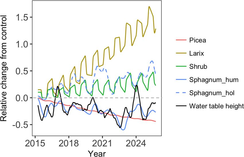
ist for non-moss PFT parameters. For example, leafcn_shrub Our model simulated two seasonal maxima of Sphagnum
is the seventh most sensitive parameter for GPP_moss, indi- moss GPP: one at the end of May and the other in August
cating that competition between the PFTs for resources may (Fig. 3). Both peaks are lower than the maximum of observed
be important. In this case, uncertainty about parameters on (flux-partitioned) GPP, which occurs in August. Based on re-
one PFT may drive uncertainties in the simulated productiv- sults of the sensitivity analysis, it could be that the base rate
ity of other PFTs. for maintenance respiration for moss is too high, causing an
underestimate of NPP and biomass, which leads to a low bias
in peak GPP.
Biogeosciences, 18, 467–486, 2021 https://doi.org/10.5194/bg-18-467-2021X. Shi et al.: Modeling the responses of Sphagnum moss to environmental changes 475
creased mortality and autotrophic respiration rate parameters
compared to the default model (Table 3), which causes the
simulations to approach steady state relatively quickly after
the 1974 disturbance. However, the sensitivity analysis also
identifies these mortality and maintenance respiration param-
eters as highly sensitive; therefore, this simulated response
is uncertain. For the shrub stem carbon, the simulated mean
from year 2012 to 2015 was 140.4 g C m−2 , slightly higher
than the observation (133.9 g C m−2 ) but well within the ob-
served range of inter-plot variability (Fig. 4c).
Figure 3. Predicted GPP (solid red line) compared with flux- 4.3 Simulated carbon cycle response to warming and
partitioned GPP (solid black line; GPP data were not used in the elevated atmospheric CO2 concentration
parameters optimization) of Sphagnum mosses for the year 2014.
The blue line is the predicted GPP corrected with the observed wa- Different PFTs demonstrated different warming responses
ter table height. The dashed black and red lines are observed and for both ambient CO2 and elevated CO2 concentration con-
modeled water table height (the dashed gray line is the hollow sur- ditions (Fig. 5). Both Larix and shrub NPP increased with
face). warming under both CO2 concentration conditions (Fig. 5b,
c, h, and i). In addition, CO2 fertilization stimulates the
growth of these two PFTs, and the fertilization effect further
During June and October, observations suggest that increases with warming (Fig. S1). In contrast, Picea NPP de-
ELM_SPRUCE overpredicts GPP. The model does limit GPP creased with warming levels (Fig. 5a and g) for both CO2
as a function of the depth of standing water on the bog sur- conditions. For Sphagnum, NPP decreased in hummocks but
face (Eq. 7). The water table height (WTH) above the bog increased in hollows with increasing temperature (Fig. 5d, e,
surface is being predicted by the model (dashed red line in j, and k). The CO2 fertilization also stimulates the growth of
Fig. 3), and while the seasonal pattern of higher water table the Picea and Sphagnum PFTs (Fig. 5a, d, e, g, j, and k). The
in the spring and lower water table in the fall agrees well total enclosure NPP for all PFTs responded differently to the
with observations (dashed black line in Fig. 3), the predicted warming only and warming with elevated CO2 (Fig. 5f and
WTH is generally too low by 5–10 cm. The modeled WTH l). The total enclosure NPP for each warming level changed
here is for hollow. We turned off the lateral transport when less under the ambient CO2 condition than those with the
there is ice on the soil layers above the water table to avoid elevated CO2 condition, and NPP decreased with warming
an unreasonable amount of ice accumulation on the frozen in most of the years under the ambient CO2 condition but in-
layers which results when there is no flow from hummock creased under the elevated CO2 condition (Fig. 5f and l). This
to hollow. Forcing the modeled GPP to respond to observed result demonstrated that the elevated CO2 scenario changes
WTH (during the period with observations) gives a pattern of the sign of the NPP warming response for the bog peatland
increasing GPP through June and July which is more consis- ecosystem.
tent with observations (blue line in Fig. 3). We do not have Compared with the ambient biomass, the biomass of black
observations for GPP earlier than June due to limitations of spruce (Picea) significantly decreased, but the biomass of
the instrumentation when the bog surface is flooded. Larix significantly increased under the greatest warming
The model simulated reasonable annual values for Sphag- treatment (+9.00 ◦ C; Fig. 6). Biomass of shrub and hollow
num NPP for the period 2014–2017 but showed much lower Sphagnum also increased but less than Larix did. The hum-
NPP compared to observation (139 vs. 288 g C m−2 yr−1 ) for mock Sphagnum biomass also showed a strong correlation
the year 2012 (Fig. 4a). Measurement uncertainties are larger with water table height at roughly a 3-month lag (the maxi-
in 2016–2017 than in earlier years, perhaps related to a new mum correlation occurs with an 82 d lag; R 2 = 0.56). NPP
measurement protocol for those years, and the model esti- is allocated instantaneously into biomass. A positive NPP
mates are within measurement uncertainty bounds for years anomaly caused by water table shifts leads to higher LAI,
2014–2017 (Griffiths et al., 2018; Norby et al., 2019). The which also increases future productivity for some amount
observed Sphagnum NPP was measured at different plots, of time even if the water table returns to normal. Sphag-
and each plot included different species abundances. As a num biomass has a 1-year turnover time in the simulation.
result, the scaled NPP includes spatial variations and uncer- This combination of effects leads to a roughly 3-month time
tainty in species distribution (Norby and Childs, 2018). lag. Due to the relative lower height of the water table in the
Simulated tree aboveground biomass is within the ob- hummock than the hollow, the simulated hummock Sphag-
served inter-plot variability (Fig. 4b). Observations suggest num was more significantly water-stressed than the hollow
an increasing trend in tree biomass which was not pre- Sphagnum as the water table height declines. This is con-
dicted by the model. The optimized parameters show in- sistent with multiple studies finding that an increase in tem-
https://doi.org/10.5194/bg-18-467-2021 Biogeosciences, 18, 467–486, 2021476 X. Shi et al.: Modeling the responses of Sphagnum moss to environmental changes
Figure 4. Predicted (red bars) Sphagnum NPP (a), aboveground tree biomass (b), and shrub stem carbon (c) compared with the observations
(black bars). Observed NPP data are based on growth of 12–17 bundles of 10 Sphagnum stems in 2012–2015 (unpublished data) and in two
ambient plots by the method described by Norby et al. (2019) in 2016–2017 (data in Norby and Childs, 2018). The Sphagnum NPP data for
the years 2015–2017 and aboveground tree biomass and shrub stem carbon for the years 2014–2015 are independent of the related parameter
optimization.
peratures associated with drought (low water table height) tent using a stand-alone photosynthesis model. In both cases,
reduces Sphagnum growth (Bragazza et al., 2016; Granath the predicted peak GPP is lower than observations. Walker
et al., 2014; Mazziotta et al., 2018). We plotted the pre- et al. (2017) were, however, able to capture the observed
dicted canopy evaporation for hummock and hollow Sphag- peak magnitude with a combination of light extinction co-
num responses to warming and found that both hummock efficient, canopy clumping coefficient, maximum SAI, and a
and hollow Sphagnum canopy evaporation amounts increase logistic function describing the effective Sphagnum SAI in
with warming for both ambient and elevated atmospheric relation to the water table. Here we used model default val-
CO2 conditions despite the Larix and shrubs growing with ues for the light extinction and canopy clumping coefficients.
warming. Moreover, the hollow Sphagnum canopy evapora- While the water table impacts Sphagnum productivity in our
tion warming response is stronger than that of the hummock simulation, modeled LAI is mainly controlled by NPP and
Sphagnum (Fig. S2). In summary, the growth of bog vegeta- turnover. In addition, we use the default formulation for the
tion is predicted to have species-specific warming responses acclimation of Vcmax in ELM which is based on a 10 d mean
that differ in sign and magnitude. growing temperature. At this point, we do not have sufficient
measurements to test this assumption, but we can prioritize
these measurements in the future. Sphagnum temperature is
5 Discussion computed from surface energy balance, but because the cur-
rent model does not estimate the shading effects from trees
Sphagnum moss is the principal plant involved in the peat ac-
and shrubs, this may be overestimated. Moreover, biases in
cumulation in peatland ecosystems, and the effective charac-
predicted water table height contribute to errors in the cal-
terization of its biophysical and physiological responses has
culated submergence effect. Improving these biases and as-
implications for predicting peatland and global carbon, wa-
suming an exponential rather than a linear CO2 uptake pro-
ter, and climate feedbacks. This study moves us closer to our
file may improve representation of the submergence effect.
long-term goal of improving the prediction of peatland water,
All these aspects may be attributed to the biases of the sim-
carbon, and nutrient cycles in ELM_SPRUCE by introducing
ulated Sphagnum GPP. We can consider this in the future
a new Sphagnum moss PFT and implementing water content
when we have more detailed measurements. Further inves-
dynamics and photosynthetic processes for this nonvascular
tigation is thus needed to understand how representative the
plant. The Sphagnum model development combined with our
chamber-based observations of the larger-scale SPRUCE en-
previous hummock and hollow microtopography represen-
closures from Walker et al. (2017) are and to reconcile these
tation and laterally coupled two-column hydrology scheme
GPP estimates with plot-level NPP observations (Norby et
enhance the capability of ELM_SPRUCE in simulating high-
al., 2019).
carbon wetland hydrology and carbon interactions and their
The hydrology cycle, especially water table depth (WTD),
responses to plausible environmental changes.
is also a key factor that influences the seasonality of GPP
5.1 Uncertainties in simulating Sphagnum productivity in Sphagnum mosses (Lafleur et al., 2005; Riutta et al., 2007,
Sonnentag et al., 2010; Grant et al., 2012; Kuiper et al., 2014;
Our predicted peak GPP is similar to the results found by Walker et al., 2017). One key feedback is that if the water ta-
Walker et al. (2017) when they calculated the internal resis- ble declines, there can be enhanced decomposition and subsi-
tance to CO2 diffusion as a function of Sphagnum water con- dence of the peat layer, which brings the surface down closer
Biogeosciences, 18, 467–486, 2021 https://doi.org/10.5194/bg-18-467-2021X. Shi et al.: Modeling the responses of Sphagnum moss to environmental changes 477 Figure 5. Predicted NPP response to warming with ambient atmospheric CO2 (a–f, solid lines) and warming with elevated atmospheric CO2 concentration (g–l, dashed lines). The solid black line TAMB is the ambient temperature and CO2 case, and T0.00 to T9.00 means increasing temperature from 0 to 9 ◦ C. to the water table again. But we currently did not consider the side the warmer plots, some disequilibration could remain. peat layer elevation changes in our model, and this will be High-frequency latent heat flux data from the site are cur- one of the future development directions. The capillary rise rently lacking but could help to constrain these effects in the plays into the Sphagnum hydrological balance, which varies future. depending on water table depth and evaporative demand. At The current phenology observations also include whether short timescales or under rapidly changing conditions, there Sphagnum hummock and hollow are wet or dry, and we may not be equilibration between the Sphagnum water con- could look at the relationship with soil water content sen- tent and the peat moisture. Generally, the Sphagnum water sors in the future. Moreover, the timescales for rewetting may content will equilibrate with the peat on a daily basis out- change as the peat dries since the cross section for capillary side the plot since the dew point is often reached at night. rise will decline, and thus the maximum flux to the surface But since the vapor pressure deficit does not go to zero in- will decline. At some point between gravity potential and re- https://doi.org/10.5194/bg-18-467-2021 Biogeosciences, 18, 467–486, 2021
478                                      X. Shi et al.: Modeling the responses of Sphagnum moss to environmental changes

                                                                    Sphagnum water content to soil water content or to water ta-
                                                                    ble depth they used for the SPRUCE site was empirical and
                                                                    may not be representative for a peatland ecosystem. To better
                                                                    represent the peatland ecosystem in our model, we will even-
                                                                    tually treat the Sphagnum mosses as the “top” soil layer with
                                                                    a lower thermal conductivity and higher hydraulic capacity
                                                                    (Beringer et al., 2001; Wu et al., 2016; Porada et al., 2016).

                                                                    5.2   Predicted warming and elevated CO2
                                                                          concentration response uncertainties

                                                                    Our model warming simulations suggested that increasing
Figure 6. The relative changes in biomass for different PFTs and    temperature reduced the Picea growth but increased the
water table height (the weighted average between hummock and
                                                                    growth of Larix under both ambient and elevated atmo-
hollow) between the +9.00 ◦ C treatment case and the ambient case
((+9.00 ◦ C / ambient) − 1).
                                                                    spheric CO2 conditions. The main reason for this model dif-
                                                                    ference in response for the two tree species is that despite
                                                                    their similar productivity under ambient conditions, Picea
                                                                    has more respiring leaf and fine root biomass because of
duced hydraulic conductivity, we expect that the capillarity        lower SLA, longer leaf longevity, and higher fine root alloca-
will no longer satisfy evaporative demand. Alternately, un-         tion. Therefore, warming results in a much larger increase in
der saturated conditions when the water table is close to the       maintenance respiration relative to changes in NPP for Picea
Sphagnum surface, Sphagnum photosynthesizing tissue can             compared to Larix (Figs. 5 and S4). Increased tree growth
become submerged or surrounded by a film of water that              and productivity in response to the recent climate warming
is likely to reduce the effective LAI of the Sphagnum and           for high-latitude forests has been reported (Myneni et al.,
thus reduce photosynthesis (Walker et al., 2017). Submerged         1997; Chen et al., 1999; Wilmking et al., 2004; Chavardes,
Sphagnum can take up carbon derived from CH4 via symbi-             2013). On the other hand, reductions in tree growth and neg-
otic methanotrophs (Raghoebarsing et al., 2005), but in any         ative correlations between growth and temperature have also
case, CO2 diffusion for photosynthesis will dramatically de-        been shown (Barber et al., 2000; Wilmking et al., 2004; Silva
crease under water. Larmola et al. (2014) also reported that        et al., 2010; Juday and Alix 2012; Girardin et al., 2016;
the activity of oxidizing bacteria provides not only carbon but     Wolken et at., 2016).
also nitrogen to peat mosses and, thus, contributes to carbon          Our model also predicted the increasing growth of shrubs
and nitrogen accumulation in peatlands, which store approx-         with increased temperature in a similar way to the simulated
imately one-third of the global soil carbon pool. We currently      increase in shrub cover caused mainly by warmer temper-
did not consider this kind of CH4 associated carbon and ni-         atures and longer growing seasons reported by Miller and
trogen uptake by Sphagnum.                                          Smith (2012) using their model LPJ-GUESS. In addition,
   The live green Sphagnum moss layer buffers the exchange          several other modeling studies have also found increased
of energy and water at the soil surface and regulates the soil      biomass production and LAI related to shrub invasion and
temperature and moisture because of its high water holding          replacement of low shrubs by taller shrubs and trees in re-
capacity and the insulating effect (McFadden et al., 2003;          sponse to increased temperatures in tundra regions (Zhang et
Block et al., 2011; Turetsky et al., 2012; Park et al., 2018).      al., 2013; Miller and Smith, 2012; Wolf et al., 2008; Porada
Currently, we apply the same method for the hummock and             et al., 2016; Rydssa et al., 2017).
hollow Sphagnum water content prediction and can test the              The responses of Sphagnum mosses to warming simu-
model against the measured data when more data are avail-           lated by ELM_SPRUCE showed that Sphagnum growth in
able. Our model still can predict Sphagnum water content            hollows was consistently higher with increased temperatures
differences between these microtopographies as expected,            when water availability was not limited. Sphagnum growing
though with the water content of hollows greater than that          on hummocks, on the other hand, showed negative warming
of hummocks. In addition, our model is able to represent            responses that are related to the strong dependency on wa-
the self-cooling effect, although we do not yet have measure-       ter table height. A recent study of the same SPRUCE site
ments available to validate the model. The relationship of the      (Norby et al., 2019) had suggested that the hummock and
differences between vegetation temperature (TV) and 2 m air         hollow microtopography had a larger influence on Sphag-
temperature (TBOT) (TV-TBOT) and canopy evaporation for             num responses to warming than species-specific traits. In ad-
both hummock and hollow Sphagnum demonstrated that the              dition, the previous studies had demonstrated that the most
differences of TV-TBOT was negative and the canopy evap-            dominant mechanism of Sphagnum warming response was
oration had a negative relationship with TV-TBOT (Fig. S3).         probably through the effect of warming on depth to the water
Moreover, Walker et al. (2017) reported that the function of        table and water content of the acrotelm, both of which re-

Biogeosciences, 18, 467–486, 2021                                                      https://doi.org/10.5194/bg-18-467-2021
X. Shi et al.: Modeling the responses of Sphagnum moss to environmental changes 479 sponded to increasing temperature (Grosvernier et al., 1997; rently disputed, with studies indicating an increase in growth Rydin, 1985; Weltzin et al., 2001; Norby et al., 2019). More- rate (Jauhiainen and Silvde 1999; Heijmans et al., 2001; over, desiccation of capitula due to increased evaporation as- Saarnio et al., 2003), decreases in growth rate (Grosvernier sociated with higher temperatures and vapor pressure deficits et al., 2001; Fenner et al., 2007), and no response (Van der can reduce Sphagnum growth independent of the water table Hejiden et al., 2000; Hoosbeek et al., 2002; Toet et al., 2006). depth (Gunnarsson et al., 2004). We currently used the same Norby et al. (2019) indicated no growth stimulation of both parameters for both hummock and hollow but could consider hummock and hollow Sphagnum under elevated CO2 con- species differences in the future. Norby et al. (2019) inves- dition but significant negative effects of elevated CO2 on tigated different Sphagnum species at the same site and re- Sphagnum NPP in the year 2018 at the same study site. Con- ported there was no support for the hypothesis that species trasting responses between Sphagnum species are thought to more adapted to dry conditions (e.g., S. magellanicum and be coupled with the water availability. In contrast, our model Polytrichum mainly on hummocks) would be more resistant results showed that both hummock and hollow Sphagnum to the stress and would increase in dominance, and both hum- growths were stimulated by the elevated CO2 concentration, mock and hollow Sphagnum decline with warming despite which may be attributed to the fact that we did not consider the differences between them. This declining trend may be the light competition between the PFTS (shrub and tree shad- in part due to increased shading from the shrub layer which ing effects) but used a fixed cover fraction of Sphagnum. expands with warming (McPartland et al., 2020). The CO2 vertical concentration profile is assumed to be Ecosystem warming can have direct and indirect effects uniform in the simulations. In the experiment, the enclosure’s on Sphagnum moss growth. The growth of Sphagnum may regulated additions of pure CO2 are distributed to a manifold be reduced directly by higher air temperature due to the rela- that splits the gas into four equal streams feeding each of the tively low temperature optima of moss photosynthesis (Hob- four air handling units (Hanson et al., 2017, Fig. 2a) and in- bie et al.,1999; Van Gaalen, 2007; Walker et al., 2017). On jects it into the duct work of each furnace just ahead of each the other hand, increased shading by the shrub canopy and blower and heat exchanger. Horizontal and vertical mixing associated leaf litter could indirectly decrease moss growth within each enclosure homogenizes the air volume distribut- (Chapin et al., 1995; Hobbie and Chapin 1998; Van der Wal ing the CO2 along with the heated air. The horizontal blowers et al., 2005; Walker et al., 2006; Breeuwer et al., 2008). In in the enclosures together with external wind eddies ensure contrast, other studies suggest that Sphagnum growth can be vertical mixing. We do not have routine automated CO2 con- promoted by a cooling effect of shading on the peat surface, centration data below 0.5 m. The moss layer may well be ex- by alleviating photo-inhibition of photosynthesis, and also by periencing higher concentrations than assumed by the model, reducing evaporation stress (Busby et al., 1978; Murray et al., but such an impact will be minimized during daylight hours. 1993; Man et al., 2008; Walker et al., 2015; Bragazza et al., Preliminary isotopic measurements imply that a significant 2016; Mazziotta et al., 2018). Our model sensitivity analysis fraction of carbon assimilated by the moss may come from also indicated that the parameters of shrub showed signifi- subsurface-respired CO2 (i.e., CO2 with older 14 C signatures cant sensitivities to Sphagnum mosses’ GPP, indicating that predating bomb carbon that can only be sourced from deeper competition between the PFTs for resources might be im- peat; Hanson et al., 2017). However, the observed elevated portant. Moreover, ELM_SPRUCE did predict the enhance- CO2 response is smaller than simulated (Hanson et al., 2020). ment of shrub and Larix tree with increased temperatures Understanding the drivers of elevated CO2 response or lack in both ambient and elevated CO2 conditions (LAI increas- thereof is a key topic for future work. ing with warming; Fig. S5). Currently, ELM_SPRUCE does To better investigate the Sphagnum warming and elevated not include light competition among multiple PFTs and thus CO2 responses, we should also focus on revealing the in- does not represent cross-PFT shading effects, which may teractions with shrub and nitrogen availability (Norby et al., contribute to the warming and elevated CO2 response differ- 2019). Nitrogen (N2 ) fixation is a major source of available ences between our model prediction and the observed result N in ecosystems that receive low amounts of atmospheric N of Norby et al. (2019). Meanwhile, we have fixed cover frac- deposition, like boreal forests and subarctic tundra (Lindo et tion for PFTs in our model which may also contribute to the al., 2013; Weston et al., 2015; Rousk and Michelsen, 2016; disagreement of predicted and observed warming responses, Kostka et al., 2016). For example, diazotrophs are estimated while Norby et al. (2019) showed that the fractional cover of to supply 40 %–60 % of N input to peatlands (Vile et at., different Sphagnum species declined with warming. 2014) with a high accumulation of fixed N in plant biomass Sphagnum mosses are sitting on top of high CO2 sources. (Berg et al., 2013). Nevertheless, N2 fixation is an energy- CH4 can be a significant carbon source of submerged Sphag- expensive process and is inhibited when N availability and num (Raghoebarsing et al., 2005; Larmola et al., 2014); the reactive nitrogen deposition are high (Gundale et al., 2011; refixation of CO2 derived from decomposition processes is Ackermann et al., 2012; Rousk et al., 2013). This could also an important source of carbon for Sphagnum (Rydin and limit ecosystem N input via the N2 fixation pathway. We are Clymo, 1989; Turetsky and Wieder, 1999). The effects of the measuring Sphagnum-associated N2 fixation at the SPRUCE elevation of atmospheric CO2 on Sphagnum moss are cur- site and found that rates decline with increasing temperature https://doi.org/10.5194/bg-18-467-2021 Biogeosciences, 18, 467–486, 2021
You can also read