Climate change over the high-mountain versus plain areas: Effects on the land surface hydrologic budget in the Alpine area and northern Italy - HESS
←
→
Page content transcription
If your browser does not render page correctly, please read the page content below
Hydrol. Earth Syst. Sci., 22, 3331–3350, 2018
https://doi.org/10.5194/hess-22-3331-2018
© Author(s) 2018. This work is distributed under
the Creative Commons Attribution 4.0 License.

Climate change over the high-mountain versus plain areas:
Effects on the land surface hydrologic budget in the Alpine area
and northern Italy
Claudio Cassardo1,2,4 , Seon Ki Park2,3,4 , Marco Galli1,a , and Sungmin O5,b
1 Department    of Physics and NatRisk Center, University of Torino “Alma Universitas Taurinorum”, Torino, Italy
2 Department    of Climate and Energy Systems Engineering, Ewha Womans University, Seoul, Republic of Korea
3 Department of Environmental Science and Engineering, Ewha Womans University, Seoul, Republic of Korea
4 Center for Climate/Environment Change Prediction Research and Severe Storm Research Center,

Ewha Womans University, Seoul, Republic of Korea
5 Institute for Geophysics, Astrophysics, and Meteorology, University of Graz, Graz, Austria
a now at: Air Force Mountain Centre, Sestola, Modena Province, Italy
b now at: Department of Biogechemical Integration, Max Planck Institute for Biogeochemistry, Jena, Germany

Correspondence: Seon Ki Park (spark@ewha.ac.kr)

Received: 18 September 2017 – Discussion started: 18 October 2017
Revised: 17 February 2018 – Accepted: 13 May 2018 – Published: 14 June 2018

Abstract. Climate change may intensify during the second           floods coincidently. Our results have serious implications for
half of the current century. Changes in temperature and pre-       human life, including agricultural production, water sustain-
cipitation can exert a significant impact on the regional hy-      ability, and general infrastructures, over the Alpine and adja-
drologic cycle. Because the land surface serves as the hub of      cent plain areas and can be used to plan the managements of
interactions among the variables constituting the energy and       water resources, floods, irrigation, forestry, hydropower, and
water cycles, evaluating the land surface processes is essen-      many other relevant activities.
tial to detail the future climate. In this study, we employ a
trusted soil–vegetation–atmosphere transfer scheme, called
the University of Torino model of land Processes Interac-
tion with Atmosphere (UTOPIA), in offline simulations to           1   Introduction
quantify the changes in hydrologic components in the Alpine
area and northern Italy, between the period of 1961–1990 and       Recent reports from the Intergovernment Panel on Climate
2071–2100. The regional climate projections are obtained by        Change (IPCC), based on the coupled atmosphere–ocean
the Regional Climate Model version 3 (RegCM3) via two              general circulation models (GCMs), on the condition of in-
emission scenarios – A2 and B2 from the Intergovernmental          creasing concentration of greenhouse gases (IPCC, 2007,
Panel on Climate Change Special Report on Emissions Sce-           2013) indicate that climate change by the end of this cen-
narios. The hydroclimate projections, especially from A2, in-      tury (e.g., increase in the mean temperature and change in
dicate that evapotranspiration generally increases, especially     the precipitation amount) is expected to occur irregularly in
over the plain areas, and consequently the surface soil mois-      space and time but to mostly affect some specific and crit-
ture decreases during summer, falling below the wilting point      ical regions (Beniston, 2006), including the vicinity of the
threshold for an extra month. In the high-mountain areas, due      Mediterranean – well known as one of the world’s climatic
to the earlier snowmelt, the land surface becomes snowless         hotspots (Giorgi, 2006; Diffenbaugh and Giorgi, 2012; Go-
for an additional month. The annual mean number of dry             biet et al., 2014; Vautard et al., 2014; Coppola et al., 2016;
(wet) days increases remarkably (slightly), thus increasing        Paeth et al., 2017). Within this region, the Alpine and adja-
the risk of severe droughts, and slightly increasing the risk of   cent areas are expected to undergo a relatively larger temper-

Published by Copernicus Publications on behalf of the European Geosciences Union.
3332                                         C. Cassardo et al.: Climate change over the high-mountain versus plain areas

ature increase (Giorgi and Lionello, 2008), which has been        have similarly for the seasonal mean temperature with higher
generally confirmed since the IPCC Fourth Assessment Re-          spread in GCMs; however, during summer, the spread of the
port (AR4; IPCC, 2007).                                           RCMs – particularly in terms of precipitation – is larger than
   In a generic mesoscale basin, such potential changes will      that of the GCMs, which indicates that the European sum-
influence hydrologic budget, thus altering the amount of          mer climate is strongly controlled by parameterized physics
available water and acting as climate feedback. Previous          and/or high-resolution processes. They also concluded that
studies conducted over the alpine areas (Giorgi et al., 1997;     the PRUDENCE results were confident because the mod-
Beniston et al., 2007; Kotlarski et al., 2015) demonstrated       els had a similar response to the given radiative forcing.
amplification of the climate change signal by topography          Déqué et al. (2007) showed that the signal from the PRU-
through local hydroclimatic and land surface feedbacks: the       DENCE ensemble is significant in terms of the minimum
snow cycle plays a key role as variations in the cycle of         expected 2 m temperature and precipitation responses. Ja-
snowpack accumulation and melting affect the generation           cob et al. (2007a) demonstrated that RCMs in PRUDENCE
of snowmelt-driven runoff. In addition, the temperature and       generally reproduce the large-scale circulation of the driving
seasonal precipitation pattern changes can affect the perma-      GCM. Coppola and Giorgi (2010) found a broad agreement,
nent or seasonal snowmelt, thus affecting streamflow tim-         in the 21st century climate projections over Italy, between
ings, groundwater recharge, and runoff, and consequently the      the results obtained from the ensembles of PRUDENCE
water availability. Even where the precipitation will increase,   and the Coupled Model Intercomparison Project (CMIP;
the concurrent warming will favor a further increase in evap-     https://cmip.llnl.gov/, last access: 15 February 2018) Phase 3
otranspiration. The decrease in water supplies, conjunctly        (CMIP3); however, the CMIP3 GCMs showed a much larger
with the likely increase in the demand, could significantly       range of bias for temperature and precipitation than the PRU-
influence agriculture (the largest consumer of water) as well     DENCE RCMs. These studies indicate that results from the
as municipal, industrial, and other uses (EEA, 2005). Never-      PRUDENCE and CMIP3/CMIP Phase 5 (CMIP5) experi-
theless, to evaluate the local net effect of changing climate     ments are roughly equivalent for the Mediterranean region
on water resources, the hydrologic budget must be detailed        and the Alpine sector.
(Bocchiola et al., 2013).                                            The GCMs represent the large-scale atmospheric and
   Seasonal variations of temperature and precipitation also      oceanic processes. Even if they include sophisticated atmo-
drive changes in runoff and streamflow: for instance, the         spheric physics and feedbacks with land surface and ocean
spring peak streamflow may occur earlier than the present         conditions, they only show conditions averaged over large
in places where snowpack significantly determines the wa-         areas. Hydrologic processes normally operate at relatively
ter availability (IPCC, 2007). Such changes may seriously         smaller scales, i.e., mesoscale and storm scale in meteorol-
influence the water and flood management, often with sig-         ogy and basin scale in hydrology, and local conditions can be
nificant economic consequences, though the resulting effects      most extreme than those suggested by the areal mean values
may differ for regions even at similar latitudes, as evidenced    (see, e.g., the analysis on the groundwater use and recharge
by Adam et al. (2009) for the high latitudes of North America     in Crosbie et al., 2005). Several recent studies attempted to
and Eurasia.                                                      evaluate the hydrologic effects of climate changes in indi-
   Usually GCMs are calculated in relatively coarse grid          vidual small-scale catchments using a variety of water bal-
spacings, thus inadequately representing the regional topog-      ance models and climate change scenarios (e.g., Nemec and
raphy and climate (Bhaskaran et al., 2012). Therefore, down-      Schaake, 1982; Gleick, 1986, 1987; Flaschka et al., 1987;
scaling of the GCM variables to regional scale is essential for   Bultot et al., 1988; Ayers et al., 1990; Lettenmaier and Gan,
a better depiction of regional climate: the dynamic downscal-     1990; Klausmeyer, 2005; Buytaert et al., 2009; Berg et al.,
ing uses the regional climate models (RCMs) with a higher         2013). Despite of some differences in results, due to the dif-
resolution (typically 10–50 km) and the same principles of        ferent forcing data or scenarios used (Rind et al., 1992), they
dynamical and physical processes as GCMs (e.g., Wilby and         have gathered some suitable information at basin or regional
Wigley, 1997; Christensen et al., 2007; Jury et al., 2015). It    scale.
is demonstrated that RCMs significantly improve the model            These studies also reveal that the land surface has been rec-
precipitation formulation (e.g., Frei et al., 2006; Gao et al.,   ognized as a critical component for the climate. Key points
2006; Buonomo et al., 2007; Boberg et al., 2009). In this         are the partitioning of solar radiation into sensible and latent
context, a project called the Prediction of Regional scenar-      heat fluxes, and that of precipitation into evaporation, soil
ios and Uncertainties for Defining EuropeaN Climate change        storage, groundwater recharge, and runoff. Despite the in-
risks and Effects (PRUDENCE; http://prudence.dmi.dk/, last        creased consideration of such processes, the land surface pa-
access: 15 September 2017) was undertaken, aiming at pro-         rameters are not systematically measured at either large scale
viding high-resolution climate change scenarios for Europe        or mesoscale, making it hard to perform hydrologic analy-
at the end of the 21st century via dynamical downscaling of       ses. To overcome such a problem, we have used a method-
global climate simulations (Christensen et al., 2007). Déqué      ology called the CLImatology of Parameters at the Surface
et al. (2005) found that, over Europe, GCMs and RCMs be-          (CLIPS), proposed by some other studies (e.g., Cassardo et

Hydrol. Earth Syst. Sci., 22, 3331–3350, 2018                                   www.hydrol-earth-syst-sci.net/22/3331/2018/
C. Cassardo et al.: Climate change over the high-mountain versus plain areas                                                3333

al., 1997, 2009). According to CLIPS, the output of a land        2.1   RegCM3
surface model (LSM) is used as a surrogate of surface obser-
vations, to estimate the surface layer parameters.                The earliest version of RegCM was originally proposed by
   The goal of this study is to investigate the effects of cli-   Dickinson et al. (1989) and Giorgi (1990) to use limited-
mate change, based on high and low emission scenarios, on         area models as a tool for regional climate studies, with the
the hydrologic components in the Alpine and adjacent areas,       aim of downscaling the GCM results. In this way, the GCM
including the Po Valley in Italy, near the end of this cen-       runs could provide the initial conditions and time-dependent
tury. Section 2 describes the details of RCM and LSM em-          boundary conditions to RCMs.
ployed in this study, and Sect. 3 describes the experiment de-       The dynamical core of RegCM3 is based on the hydro-
sign. Results concerning the hydrologic budget are reported       static version of the National Center for Atmospheric Re-
in Sect. 4, and conclusions are provided in Sect. 5.              search/Pennsylvania State University Mesoscale Model ver-
                                                                  sion 5 (MM5: Grell et al., 1994). The RegCM is a hydro-
                                                                  static and compressible primitive equation model with a σ
2   Description of the models                                     vertical coordinate. More details on RegCM3 are referred
                                                                  to in the MM5 documentation (Grell et al., 1994) and some
In this study, calculation of the future hydrologic budget        papers describing previous versions of RegCM (e.g., Giorgi
components has been performed through the University of           et al., 1993; Giorgi and Shields, 1999). The RegCM3 is doc-
Torino model of land Processes Interaction with Atmosphere        umented in Elguindi et al. (2007).
(UTOPIA; Cassardo, 2015): meteorological inputs to drive             The RegCM3 includes several physical process packages.
UTOPIA under the current and future climate conditions            Precipitation involves both grid- and subgrid-scale processes
are obtained from the Regional Climate Model version 3            (e.g., Pal et al., 2000), which are crucial as a source of er-
(RegCM3). Since the details of the RegCM3 run have already        rors in climate simulations (e.g., Nakicenovic and Swart,
been published (Giorgi et al., 2004a, b; Gao et al., 2006),       2001). The implemented subgrid precipitation schemes are
here a short description of RegCM3 will be given. Regard-         described in Anthes (1977), Emanuel (1991), Giorgi (1991),
ing UTOPIA, just some portions relevant for this study are        Grell (1993), and Emanuel and Živković-Rothman (1999).
described.                                                        The physics of the surface processes is described accord-
   Despite the availability of the products for Europe within     ing to the Biosphere–Atmosphere Transfer Scheme (BATS)
the World Climate Research Program COordinated Re-                manual (Dickinson et al., 1993). Subgrid differences in to-
gional Downscaling EXperiment (EURO-CORDEX; http:                 pography and land use are taken into account using a mosaic-
//www.euro-cordex.net/, last access: 5 February 2018),            type approach (Giorgi et al., 2003b). Two kinds of water
which includes a newer version of RegCM (i.e., RegCM4),           bodies are considered – open (e.g., oceans) and closed (e.g.,
we decided to employ RegCM3 for the following rea-                lakes).
sons: (1) RegCM3 had been employed in several impor-                 The open-water bodies are described by the water tem-
tant projects, including PRUDENCE, ENSEMBLES (http://             perature, introduced as a boundary condition for the model.
ensembles-eu.metoffice.com/, last access: 5 February 2018),       The closed ones are treated as the open bodies, or using a
and the Central and Eastern europe Climate change Im-             specific one-dimensional lake model interacting in two ways
pact and vulnerabiLIty Assessment (CECILIA; http://www.           with the atmosphere (Hostetler and Bartlein, 1990). Aerosols
cecilia-eu.org/, last access: 5 February 2018), whose outputs     and chemical compounds are considered, accounting for their
had been used in numerous studies focusing on Europe (e.g.,       diffusion and removal processes, as well as the radiative ef-
Blenkinsop and Fowler, 2007; Christensen and Christensen,         fects; details about the RegCM3 chemistry are found in Qian
2007; Ballester et al., 2010; Coppola and Giorgi, 2010; Her-      et al. (2001), Giorgi et al. (2003a), and Solomon et al. (2006).
rera et al., 2010; Rauscher et al., 2010; Kyselý et al., 2011;       The RegCM3 has been employed and tested in various
Torma et al., 2011; Heinrich et al., 2014; Skalák et al., 2014;   contexts, on various space scales, for a broad range of sci-
Faggian, 2015); (2) RegCM3 had also been widely used,             entific problems, including climate change (Giorgi et al.,
even most recently, for the studies of climate projections,       2004a, b; Diffenbaugh et al., 2005; Gao et al., 2006), air qual-
model evaluations, and sensitivities over the target areas in     ity (Solomon et al., 2006), water resources (Pal and Eltahir,
our study – the Alpine and adjacent areas (e.g., Gao et al.,      2002), extreme events (Pal et al., 2004), agriculture (White
2006; Smiatek et al., 2009; Coppola and Giorgi, 2010; Im et       et al., 2006), land cover change (Abiodun et al., 2007), and
al., 2010; Coppola et al., 2014; Nadeem and Formayer, 2016;       biosphere-atmosphere interactions (Pal and Eltahir, 2003).
Alo and Anagnostou, 2017); (3) since plenty of model out-
puts were available from several relevant projects (e.g., PRU-
DENCE, ENSEMBLES, CECILIA, etc.) and we had limited
resources for exploring all available data sources, we decided
to select a well-known model which had been extensively
used for such kind of studies.

www.hydrol-earth-syst-sci.net/22/3331/2018/                                    Hydrol. Earth Syst. Sci., 22, 3331–3350, 2018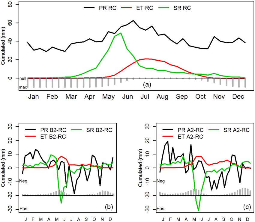
3334                                          C. Cassardo et al.: Climate change over the high-mountain versus plain areas

2.2    UTOPIA                                                       model. Examples of its use can be found in several stud-
                                                                    ies. Ruti et al. (1997) compared LSPM and BATS in the
The UTOPIA is a diagnostic one-dimensional model, for-              Po Valley, Italy. Cassardo et al. (1998) studied its depen-
merly named the Land Surface Process Model (LSPM; Cas-              dence on initialization. Cassardo et al. (2005) used LSPM
sardo et al., 1995; Cassardo, 2006). It can be used on a stand-     to study surface energy and hydrologic budget on the syn-
alone basis or be coupled with an atmospheric circulation           optic scale. Cassardo et al. (2002, 2006) used the LSPM to
model or an RCM, serving as the lower boundary condition.           analyze extreme flood events in Piedmont, Italy. In Cassardo
All specific details about its use and features are fully de-       et al. (2007), LSPM has been used to study the 2003 heat
scribed in Cassardo (2015).                                         wave in Piedmont. Studies with LSPM on non-European cli-
   The land surface processes in UTOPIA are described in            mates have also been accomplished, related to very dry sites
terms of physical fluxes and hydrologic states of the land.         (Feng et al., 1997; Loglisci et al., 2001), to the onset of the
The former includes radiation fluxes, momentum fluxes, sen-         Asian monsoon (Cassardo et al., 2009), and to the soil tem-
sible and latent energy fluxes, and heat transfer in multi-layer    perature response in Korea to a changing climate (Park et al.,
soil, while the latter includes snow accumulation and melt,         2017). The UTOPIA was also coupled with the Weather Re-
rainfall, interception, infiltration, runoff, and soil hydrology.   search and Forecast (WRF) model, version 3, and applied to a
All the fluxes are computed using an electric analogue for-         flash flood caused by a landfall typhoon, as well as to the ex-
mulation, in which the fluxes are directly proportional to the      ceptionally wet period 2008–2009 in the northwestern Italy
gradients of the related scalars and inversely proportional to      (Zhang et al., 2009, 2011). Recent applications include stud-
the adequate resistance.                                            ies on the parameterization of soil freezing (Bonanno et al.,
   The UTOPIA domain is vertically subdivided into three            2010), and the cold spells over the Alpine area and the Po
main zones – the soil, the vegetation, and the atmospheric          Valley (Galli et al., 2010). It has also been applied to stud-
layer within and above the vegetation canopy layer. Variables       ies on vineyards environment, including canopy resistance
are mainly diagnosed in the soil and in the vegetation layers.      (Prino et al., 2009), energy and hydrologic budgets (Francone
The canopy itself is represented as a single uniform layer          et al., 2010), sensitivity to vegetation parameters (Francone
(i.e., big leaf approximation), whose properties are described      et al., 2012a), and an analysis of turbulence (Francone et al.,
by vegetation cover and height, leaf area index, albedo, min-       2012b).
imum stomatal resistance, leaf dimension, emissivity, and
root depth. The soil state is described by its temperature and
moisture content. These variables are calculated by the in-         3   Experimental design
tegration of the heat Fourier equation and conservation of
water mass equation using a multi-layer scheme. The main            The goal of this study is to evaluate the components of the
parameters include thermal and hydraulic conductivities, soil       surface hydrologic budget on a mesoscale area from a cli-
porosity, permanent wilting point, dry heat capacity, surface       matic point of view, and to compare the effects of the cli-
albedo, and emissivity. The UTOPIA can have as many soil            mate change on these values. Two 30-year periods have been
layers as a user specifies; however, a sufficient number of         considered: the first one (1961–1990) is the baseline pe-
layers is required for numerical stability. Note that numer-        riod or reference climate (RC), whereas the other is the last
ical stability is strictly related to the integration time step –   30 years of the 21st century (2071–2100), named the future
the model becomes unstable and blows up eventually with an          climate (FC) here. The period 1961–1990 has been employed
inadequately large time step. This is particularly true in the      in numerous previous studies on climate change projections
presence of strong moisture gradients, which could lead to          and impacts, even very recently (e.g., Giorgi and Lionello,
errors in the representation of soil moisture profiles.             2008; Smiatek et al., 2009; Ciscar et al., 2011; Kyselý et
   Finally, the presence of snow is parameterized with a sin-       al., 2011; Torma et al., 2011; Heinrich et al., 2014; Perez
gle layer assumption. Snow can cover vegetation and bare            et al., 2014; Skalák et al., 2014; Belda et al., 2015; Dunford
soil separately and possesses its proper energy and hydro-          et al., 2015; Faggian, 2015; Casajus et al., 2016; Harrison
logic budgets, thus interacting with the other components.          et al., 2016; Gang et al., 2017; Paeth et al., 2017). It had
   The UTOPIA is a diagnostic model; thus, some observa-            also been used in various climate projection projects using
tions in the atmospheric layer are required as boundary con-        GCMs and/or RCMs, such as CMIP3/CMIP5, PRUDENCE,
ditions, including air temperature, humidity, pressure, wind        ENSEMBLES, and CECILIA.
speed, cloud cover, longwave and shortwave incoming ra-                The climate projections are obtained through the IPCC
diation, and precipitation rate. Usually these observations         Special Report on Emissions Scenarios (SRES) A2 and B2
are measured values, along with the reconstruction of some          emission scenarios (Nakicenovic and Swart, 2001). Note
missing data using adequate interpolation techniques.               that the A2 scenario assumes large increases in popula-
   The UTOPIA, as well as its predecessor LSPM since 2008,          tion and economical development while the B2 scenario as-
has been tested with field campaigns and measured data ei-          sumes more sustainability and consequent smaller increases
ther by itself or as coupled with an atmospheric circulation        in those; thus, the concentration of carbon dioxide are pro-

Hydrol. Earth Syst. Sci., 22, 3331–3350, 2018                                    www.hydrol-earth-syst-sci.net/22/3331/2018/
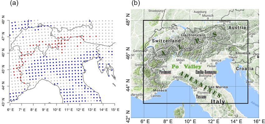
C. Cassardo et al.: Climate change over the high-mountain versus plain areas                                                3335

jected to be higher for A2 than for B2. The future climates       possible climate projections. O’Sullivan et al. (2016) found
based on the A2 and B2 scenarios are hereafter referred to as     that future summers had the largest projected warming un-
FCA2 and FCB2 , respectively.                                     der RCP 8.5 while future winters had the greatest warming
   In the last decade, numerous studies on climate projec-        under A1B and A2. Nolan et al. (2017) created a medium-
tions and impacts have been conducted using the SRES sce-         to-low emission ensemble using the RCP4.5 and B1 scenario
narios, which were the base scenarios in the CMIP3 exper-         simulations and a high emission ensemble using the RCP8.5,
iments. After the emergence of new scenarios – Represen-          A1B, and A2 simulations, which enabled 25 high and 21
tative Concentration Pathways (RCPs; Moss et al., 2010),          medium-to-low emission ensemble comparisons: they found
which were employed in the IPCC Fifth Assessment Re-              significant projected decreases in mean annual, spring, and
port (AR5; IPCC, 2013) and the CMIP5 experiments, there           summer precipitation amounts – largest for summer, with dif-
have been many studies either to check similarities and/or        ferent reduction ranges for different scenario ensembles.
differences between the two scenario sets for a given projec-        Furthermore, the SRES scenarios by themselves have of-
tion period (e.g., Riahi et al., 2011; Ward et al., 2011; Ro-     ten been adopted in most recent studies, even long after the
gelj et al., 2012; Matthews and Solomon, 2013; Baker and          release of the RCP scenarios, because the old scenarios were
Huang, 2014) or to address the value of using both scenario       in accord with their objectives (e.g., Dunford et al., 2015;
sets for future climate projections (e.g., Peters et al., 2013;   Jaczewski et al., 2015; Kiguchi et al., 2015; Kim et al.,
O’Sullivan et al., 2016; Nolan et al., 2017).                     2015; Casajus et al., 2016; Harrison et al., 2016; Mamoon et
   It turns out that both SRES and RCP scenarios are gen-         al., 2016; Stevanović et al., 2016; Tukimat and Alias, 2016;
erally in good agreements, for pairs of closest counterparts,     Zheng et al., 2016; Hassan et al., 2017; Park et al., 2017; da
in projecting climate in the 21st century. For example, Ri-       Silva et al., 2017). We employed the SRES marker scenar-
ahi et al. (2011) mentioned that SRES A2 was comparable           ios because of their long-term consistency in assessing the
to RCP 8.5. Ward et al. (2011) found that the RCP 4.5 and         impact of climate change on global and regional factors of
SRES B1/A1T scenarios were broadly consistent with the            socioeconomy and environment during the last decade – in-
fossil fuel production forecasts. Rogelj et al. (2012) pointed    cluding air quality (Jacob and Winner, 2009; Carvalho et al.,
out that the RCP scenarios spanned a larger range of tempera-     2010), water quality and resources (Wilby et al., 2006; Shen
ture estimates than the SRES scenarios, and indicated similar     et al., 2008, 2014; Luo et al., 2013), energy (Hoogwijk et al.,
temperature projections for pairs between the two scenario        2005; van Vliet et al., 2012), agriculture and forestry (Lavalle
sets: RCP 8.5 similar to A1FI, RCP6 to B2, and RCP 4.5 to         et al., 2009; Calzadilla et al., 2013; Stevanović et al., 2016;
B1, respectively. Matthews and Solomon (2013) showed that         Zubizarreta-Gerendiain et al., 2016), fisheries (Barange et al.,
the cumulative CO2 emission and corresponding warming in          2014; Lam et al., 2016), health and disease (Patz et al., 2005;
the short term (2030) are approximately the same across all       Giorgi and Diffenbaugh, 2008; Ogden et al., 2014), climate
emission scenarios, whereas those in the longer term (2100)       and weather extremes (Déqué, 2007; Marengo et al., 2009;
are similar between close counterparts of the selected SRES       Jiang et al., 2012; Rummukainen, 2012), wildfires (Liu et
and RCP scenarios: A1FI to RCP 8.5, A1B to RCP 6, and B1          al., 2010; Westerling et al., 2011), ecosystems and biodiver-
to RCP 4.5, respectively. Baker and Huang (2014) reported         sity (Araújo et al., 2008; Feehan et al., 2009; Jones et al.,
a common drying trend, over the Mediterranean region, be-         2009; Fronzek et al., 2012; Walz et al., 2014), and so forth.
tween the CMIP3 simulations based on SRES A1B and the             Although an ensemble approach with all possible scenarios
CMIP5 simulations based on RCPs 4.5 and 8.5. It is also indi-     would increase the spread of hydrologic budget simulations,
cated by Cabré et al. (2016) that SRES A2 has similarities to     due to the limited resources, we decided to select two repre-
RCP 8.5 in terms of radiative forcing, future trajectories, and   sentative marker scenarios: A2 as the higher-end and B2 as
changes in global mean temperature. In Rogelj et al. (2012),      the lower-end emission scenario, respectively.
differences in warming rates existed between the two sce-            Simulations of RegCM3 for the two periods (i.e., 1961–
nario sets due to different transient forcings; however, with a   1990 and 2071–2100) are fully referenced in Giorgi et al.
30-year average for each scenario as in our study, the results    (2004a, b) and Gao et al. (2006), and have been chosen for
and conclusions of using the SRES A2/B2 scenarios would           this study because they are still among the highest-resolution
not be significantly different from those of using the closest    datasets currently available. As shown in Coppola et al.
RCP counterparts.                                                 (2016), the RCM outputs with high resolution can allow the
   To obtain a broad range of projections, Peters et al. (2013)   hydrologic cycle to be efficiently reconstructed at a large-
projected global warming through all available emission           basin scale, even in an orographically complex area such as
scenarios, showing that RCP 8.5 and SRES A1FI and A2              the Alps.
lead to the highest temperature projections. Most recently,          The domain for this study involves most of the Alpine re-
O’Sullivan et al. (2016) and Nolan et al. (2017) assessed         gion and the Po River basin, as shown in Fig. 1. It is bordered
impacts of climate change on temperature and rainfall, re-        by the meridians 5 and 15◦ E and the parallels 43 and 48◦ N.
spectively, by the mid-21st century in Ireland using both         We have chosen this domain for two main reasons: (1) the
the SRES and RCP scenarios, and provided a wide range of          Alps represent a critical environment that already answered

www.hydrol-earth-syst-sci.net/22/3331/2018/                                    Hydrol. Earth Syst. Sci., 22, 3331–3350, 2018

3336                                         C. Cassardo et al.: Climate change over the high-mountain versus plain areas

most effectively to the recent climate warming (e.g., Benis-      to avoid any problem in interpretation of results due to the
ton, 2006); and (2) the Alps are the source of the longest and    differences in vegetation, and (2) for the “future climate”,
greatest European rivers (e.g., Rhyne, Rhone, Danube, Inn,        to alleviate the uncertainty in vegetation type at the end of
Arc, Po, etc.). Under these considerations, it is essential to    21st century. With regard to meteorological variables, this
evaluate potential changes in the soil variables and the hy-      is not a bad assumption because most observation stations
drologic budgets, induced by climate change.                      are normally installed over short grasses. Moreover, consid-
   The RegCM3 outputs are provided on a Lambert grid, with        ering plant height, root depth, and vegetation characteristics,
a 20 km spatial resolution, containing 720 land grid points       short grasses can be roughly regarded as most common cere-
on the analyzed domain (Fig. 1). The domain is divided            als (wheat, maize, etc.), and would not be quite different from
into three sets of grid points in terms of elevation: (1) one     such kind of agricultural products. Finally, we have also per-
representing the plain or low-hill areas lower than or equal      formed simulations using the “true” vegetation (as deduced
to 500 m above sea level (a.s.l.), occupying 34 % (blue);         by detailed databases), and the results with the pastures and
(2) another depicting normal mountains between 500 and            agricultural areas have generally been confirmed, though the
2000 m a.s.l., occupying 57 % (grey); and (3) the other be-       numerical values of the variables were slightly different (not
longing to the high-mountain areas higher than 2000 m a.s.l.,     shown).
occupying 9 % (red). In this study, among all the possible           Although UTOPIA could be driven by the real observa-
outputs available from UTOPIA, we give particular atten-          tions in RC, it is driven by the RegCM3 output in order
tion to the state of soil moisture and the components of hy-      to keep consistency among the RC and FC simulations and
drologic budget – precipitation, evapotranspiration, drainage,    to exclude any possible source of errors caused by differ-
and runoff. Note that some of those values were already in-       ences in input data, irregularity of grid, and/or interpolation
cluded in the RegCM3 output database. However, the land           of missing observations. In this way, we can compare the FC
surface model of RegCM3 employs an old force-restore              representations with an analogous RC representation. Thus,
method included in the BATS scheme which was demon-               here the RegCM3 outputs for each grid point have been used
strated to be insufficient to properly evaluate hydrologic bud-   as if they were observed data.
get (Ruti et al., 1997). Therefore, we made an offline run with      All RegCM3 outputs were available with a time resolu-
UTOPIA in order to allow a more realistic evaluation of the       tion of 3 h, and used as input data to UTOPIA. In order to
soil and budget components, and to have a self-consistent set     ensure numerical stability of the UTOPIA simulations, these
of variables in equilibrium among themselves.                     input data, except precipitation, have been interpolated at a
   The UTOPIA has been driven using the following output          rate of one datum per hour: we applied a cubic spline (Bur-
of RegCM3 over each grid point of the domain – precipi-           den and Faires, 2004) to the non-intermittent variables like
tation; short- and longwave radiation; and temperature, hu-       temperature, humidity, and radiation (flux). The intermittent
midity, pressure and wind at surface (i.e., the lowest level      variable like precipitation was simply redistributed to keep
of RegCM3). This procedure has been used for all three cli-       its sum, assuming a constant rate: the input data of precipi-
mates (RC, FCA2 , and FCB2 ).                                     tation were the precipitation cumulated over the timesteps of
   The UTOPIA has been configured to represent 10 soil lay-       the RCM output, and could not be interpolated with splines.
ers, following Meng and Quiring (2008), who suggested the         Although we could have converted precipitation to precipi-
use of multiple soil layers to represent well the vertical het-   tation rates, interpolated them using splines, and then recon-
erogeneity in soil properties. The thickness of soil layers       verted to cumulated precipitation over the smaller timestep
starts from 5 cm in the top layer, then doubles for every layer   of UTOPIA, the result of such a complicated procedure was
going to higher depths. The last layer must be interpreted        almost equivalent to using the method employed here. Re-
as a boundary relaxation zone. The soil characteristics have      garding radiation and wind components, we used the splines
been taken from the ECOCLIMAP database (Masson et al.,            for the sake of uniformity with other variables. Then, we fur-
2003). No soil-freezing scheme is used, and initial values of     ther controlled some unrealistic values (e.g., negative radia-
soil moisture and temperature have been set following Cas-        tions): we controlled the daily means (or cumulated values)
sardo (2015).                                                     from input (from RegCM3) and output (for UTOPIA) of the
   In terms of vegetation, short grasses are assumed to cover     interpolation to be non-negative values.
the whole domain. Actually the domain includes the Alps,             In this study, we employed a single-model approach that
the Apennines, off-alpine and hilly areas, and plains; thus,      has relatively larger uncertainty: it is desirable to employ an
there is a wide range of vegetation. Regarding plains and         ensemble approach, using multiple models and/or initial con-
hilly areas, vegetation includes pastures, grasslands, and        ditions, to estimate the range of climate projections. Our de-
some forested areas: mountain areas are mostly covered by         cision to employ the single-model approach is mainly due
trees, and the highest parts are without vegetation or covered    to limitations in resources to perform multi-model ensem-
by permanent ice (few grid points). We decided to set the         ble simulations for both the RCM and land surface model.
vegetation type equal for all grid points (i.e., short grasses)   Given such limitations, a high-resolution single model is
for the following reasons: (1) for the “reference climate”,       often an alternative choice, especially over a complex ter-

Hydrol. Earth Syst. Sci., 22, 3331–3350, 2018                                  www.hydrol-earth-syst-sci.net/22/3331/2018/
C. Cassardo et al.: Climate change over the high-mountain versus plain areas                                                               3337

Figure 1. Computational domain with grid points (a) and geographic map (b) with boundary of the study area (black solid lines). Grid points
represent, in terms of the grid elevation (h), the plain area (h ≤ 500 m a.s.l.; blue), the normal mountains (500 < h ≤ 2000 m a.s.l.; grey), and
the high-mountain area (h > 2000 m a.s.l.; red). The map on the right panel is modified from Google Maps.

rain. Coppola and Giorgi (2010) made a fine-scale (20 km)                  ences between FCs and RC; the PR difference (1PR) repre-
single-model experiment using RegCM3 and found that both                   sents PRFC minus PRRC , where FC is either FCB2 or FCA2 –
the temperature and precipitation changes via RegCM3 were                  similarly to 1ET and 1SR.
in line with the CMIP3 and PRUDENCE ensemble results.                         In this study, SM is defined as the quantity of water con-
Generally speaking, multi-model ensembles tend to decrease                 tained in soil that is composed of solid particles, air, and wa-
the errors compared to an individual model; however, due                   ter, and it is represented as saturation ratio (S):
to the averaging operation (e.g., ensemble mean), the spa-
tial and temporal variability of the signal tends to decrease.                      Vw      Vw
                                                                           S=             =    ,                                             (1)
Moreover, many previous studies on various climate change                         Vw + Va   Vv
impacts and projections had been performed using the single-
                                                                           where Vw , Va , and Vv are the volumes of water, air, and voids,
model approach (e.g., Dankers and Feyen, 2008; Beniston,
                                                                           respectively, in soil.
2009; Im et al., 2010; Krüger et al., 2012; Zanis et al., 2012;
Tainio et al., 2013; Park et al., 2017).
   The multiple simulations performed for RC and FCs are                   4     Results and discussion
presented in terms of the temporal and spatial variability by
displaying time series (annual cycles) and two-dimensional                 In this section, we provide analyses on temporal variability
maps, respectively, of the mean values of some variables.                  and spatial distribution of hydrologic budget components,
For time averaging, Xu and Singh (1998) suggested using                    making comparisons between RC and FCs. The potential
monthly mean values for discussing the hydrologic budget                   change in dryness (wetness) is also assessed through the pro-
variations induced by climate change; however, we preferred                jection of the number of dry (wet) days. Finally, we compare
a period of 10 days to better quantify time shifts of the phys-            our findings with relevant previous studies, and discuss con-
ical variables. In this study, the annual cycles are figured via           sistency and uniqueness of our study.
the 10-day averages over the 30-year simulation period, at
each elevation-categorized grid-point set. Each month has                  4.1    Temporal variability of evapotranspiration,
three 10-day periods: days 1 to 10, 11 to 20, and 21 to the                       precipitation, runoff and soil moisture
end of the month.
   The analyzed variables include precipitation (PR), evap-                Figure 2 compares the annual cycle of PR, ET, and SR in
otranspiration (ET), surface runoff (SR), and soil moisture                the plain area (h ≤ 500 m a.s.l.). In the RC summer, ET ex-
(SM). We noticed that the general trends of annual cycles are              ceeds PR from the end of June (when ET peaks to about
similar between RC and FCs. Therefore, in order to accentu-                22 mm) to the end of August (when SM is minimal around
ate the extent and direction of changes, the future variations             0.52 m3 m−3 ; see Fig. 3). PR shows its minimum between
in the hydrologic budget components are shown as the differ-               mid-June and August, when it is lower than ET. In the RC
                                                                           winter, PR is much higher than ET, and SR exceeds ET from

www.hydrol-earth-syst-sci.net/22/3331/2018/                                               Hydrol. Earth Syst. Sci., 22, 3331–3350, 2018
3338 C. Cassardo et al.: Climate change over the high-mountain versus plain areas
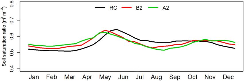
Figure 3. Annual cycles of the 10-day average values of SM, ex-
pressed as saturation ratio (in m3 m−3 ), at the soil surface layer (a
depth of 0.05 m) in RC, FCB2 , and FCA2 for the plain area.
(late May–mid-November): the driest points are antedated
by ∼ 10 days in FCs, still being in August, and their val-
ues decrease by ∼ 0.1 m3 m−3 . The decrease begins already
in spring (from late May) and continues till late October
(FCB2 ) or early November (FCA2 ), with the largest depletion
in early August (FCB2 ) and in early to mid-August (FCA2 ).
Figure 2. Annual cycles of the 10-day average values of the sur- Moreover, the period that future SM values are lower than
face hydrologic budget components for the plain area for (a) RC, the lowest SM of RC (i.e., ∼ 0.52 m3 m−3 in mid-August)
(b) FCB2 − RC, and (c) FCA2 − RC. Here, PR is precipitation, ET extends from early July to early September in FCB2 and to
evapotranspiration, and SR surface runoff. Units are millimeters mid-September in FCA2 . In the driest periods of FCs, several
(mm). grid points in the plains go below their permanent wilting
points (PWPs), which vary according to soil type, or remain
below PWP for an excessive duration by about 1 month. Our
October to March. In the summers of FCs, ET exceeds PR for results regarding the future changes in SM in the warm pe-
a longer period (in FCA2 ), and both scenarios show larger wa- riod – an increase in days of SM lower than the lowest SM
ter deficits in July and August, with the PR minimum shifted of RC, and a surplus of period below PWP – signify that,
to August in FCA2 (not shown). Furthermore, the ET max- if the land use of the grid points is pasture, we need appro-
ima shift towards July–August, in both FCA2 and FCB2 (not priate countermeasures to ensure an adequate productivity.
shown), and the values increase by as much as 3–5 mm (i.e., During the cold period in plains, SM shows the highest val-
1ETs). ues (∼ 0.73 m3 m−3 ) in both RC and FCs; the SM values of
It is conspicuous that the summer PR decreases in the FCs slightly exceed those in RC, due to the small increments
future – between the end of May and the beginning of of PR in this period (see Fig. 2b and c).
September in FCB2 (Fig. 2b), and between July and Septem- Figure 4 shows the annual cycle of hydrologic budget
ber in FCA2 (Fig. 2c). On the contrary, PR generally in- components over the high-mountain area (h > 2000 m a.s.l.).
creases in winter, between December and February, in both In both RC and FCs, PR does not exceed ET, while the gap
FCs. In autumn, 1PRs show large variations in short pe- between the two variables narrows in the FC summers, due
riods: for instance, in FCB2 , it varies as much as −6 mm to an increase in ET and a decrease in PR. In RC, ET peaks
in mid-September, +10 mm in late September, −12 mm in in mid-July while PR peaks in late June. The peak of SR,
late October, +15 mm in mid-November, and −7 mm in late between May and June, is out of phase because it is also
November. Regarding 1ET, there are almost no variations in affected by the concurrent snowmelt. It is noteworthy that
cold months, while there is a small increment (up to 3 mm) PRs in summer and autumn generally decrease in FCs (i.e.,
between April and September in FCB2 , and a larger incre- 1PR < 0) from mid-June to mid-November: except for short
ment in the same period in FCA2 , with the largest value in terms in early July, from mid- to late August, and from late
August (∼ 5 mm). This large variation in PR is partly due to September to late October in FCB2 , and except only from
the orographic effect. As reported by Gao et al. (2006), in early October to early November in FCA2 . On the contrary,
winter the southwesterly flow increases across the Alps, and in winter and spring, PRs generally increase in FCs from
causes a maximum of precipitation increase over the south- mid-January to early June except for short-term decreases in
ern Alps; in autumn the main circulation change is in the mid-April and mid-May. Regarding 1ET, there are almost no
easterly and southeasterly direction. variations in cold months, as expected (due to snow cover),
Figure 3 shows the 10-day mean values of SM for the plain whereas there is a large increment (∼ 10 mm) between May
area, expressed as saturation ratio – see Eq. (1). Variations of and June, and a low-to-moderate increment (∼ 2–6 mm) be-
SM in plains are almost negligible in a colder period (late tween July and October in FCs.
November–mid-May), but are large during a warmer period
Hydrol. Earth Syst. Sci., 22, 3331–3350, 2018 www.hydrol-earth-syst-sci.net/22/3331/2018/C. Cassardo et al.: Climate change over the high-mountain versus plain areas 3339
Finally, for 1SR in high mountains, there is a weak in-
crease (< 5 mm) between late November and late March, a
stronger increment (∼ 10 mm) in April, especially in FCB2 ,
a strong decrease (up to −25 to −31 mm) between May and
June, and a general weak decrease in summer between July
and September (see Fig. 4b and c). As a result, the maxima of
SR in FCs significantly decrease and their occurrence dates
shift ahead to May for FCB2 and between April and May
for FCA2 because snowmelt occurs nearly 30–40 days ear-
lier (see Cassardo et al., 2018) – see also the analysis on
frost frequency in Galli et al. (2010). Coppola et al. (2016)
also reported that, regarding the 75th percentile in the Alpine
areas, the snowmelt-driven runoff timing moves earlier by
about 35 days – due to the largest decrease in snow cover be-
tween April and June, sustaining the spring runoff maximum.
Those variations in our result are in line with the changes
in snowpack in FCs, which starts to melt earlier, between
late April and early May. We should consider that changes
in snow cover affect the surface energy budget through the
Figure 4. Same as in Fig. 2 but for the high-mountain area. Grey
snow–albedo feedback mechanism (Giorgi et al., 1997); that
bars at the lower portion in (a) represent the snow cover (in m) in RC
is, a reduction of snow cover decreases the surface albedo varying from 0 m (null) to 1 m (max); in (b) and (c) the snow cover
and thus increases the absorption of solar radiation at the sur- difference (in m) between the corresponding FC and RC varies from
face, resulting in warming. Moreover, soil temperature starts −1 m (Neg) to 1 m (Pos). The periods of snow ablation (late spring)
rising earlier in the year in the snowless areas. Our results and accumulation (mid or late autumn) are well identified.
also agree with other studies, carried out using RCMs over
the Alpine areas: for example, Lautenschlager et al. (2008)
for PR and ET, and Jacob et al. (2007b) for snow. Note that
SR in RC is almost null between mid-December and March
while 1SRs in FCs in the same period are positive: this in-
dicates the presence of rainfall and/or snowmelt over at least
some parts of the high-mountain grid points, even in the cold-
est periods.
Figure 5 shows SM at the high-mountain grid points and
demonstrates the effects of hydrologic budget components Figure 5. Same as in Fig. 3 but for the high-mountain area.
on surface SM. We note that the behaviors of SM in high
mountains are substantially different from those over plains
(cf. Fig. 3). In RC, the highest SM (∼ 0.65 m3 m−3 ) occurs 4.2 Spatial distribution of evapotranspiration,
in early June while the lowest SM (∼ 0.51 m3 m−3 ) arises in precipitation, runoff and soil moisture
early to mid-March. The increase in SM from late March to
early June is related to snowmelt due to an increase in net Our analyses illustrate that the differences in the SM behav-
radiation. Surface SM in RC starts to decrease as the cold iors between RC and FC, both over plains (Fig. 3) and in
season starts in early November, reaching the minimum in high mountains (Fig. 5), are strongly linked to the variations
mid-March. Note that SMs during the same cold period in in the hydrologic budget components. In this section, to un-
FCs are larger than SM in RC, evidencing a larger amount derstand such linkage more clearly, we perform analyses on
of liquid precipitation in FCs: in other words, winter rain- the spatial distribution of hydrologic variables (i.e., PR, ET,
fall will be more frequent in the future. The peak of SM in SR, and surface SM) along with discussions on the associ-
spring is advanced by 10–20 days in FCs, occurring in early ated energy variables (i.e., net radiation, NR, and surface soil
May. The magnitude of maximum SM in FCs is a bit lower temperature, ST), during summer when such variables gen-
than that in RC but the spread is larger, implying that snow erally show their largest values. Details in the analyses of NR
ablation starts much earlier and lasts longer. In addition, the and ST are referred to Cassardo et al. (2018).
occurrence of the minimum SR shifts from mid-March in RC Figure 6 shows the variables averaged in the month of July,
to summer in FCs: in both February and early August (i.e., in which PR and surface SM are close to their annual minima
two minima) in FCB2 , and late August in FCA2 . This shifting while ET is close to its annual maximum. Here, we discuss
is mainly caused by the enhancement of ET. the variables in terms of anomalies of FCA2 only because of
similar patterns to but larger variations than those of FCB2 .
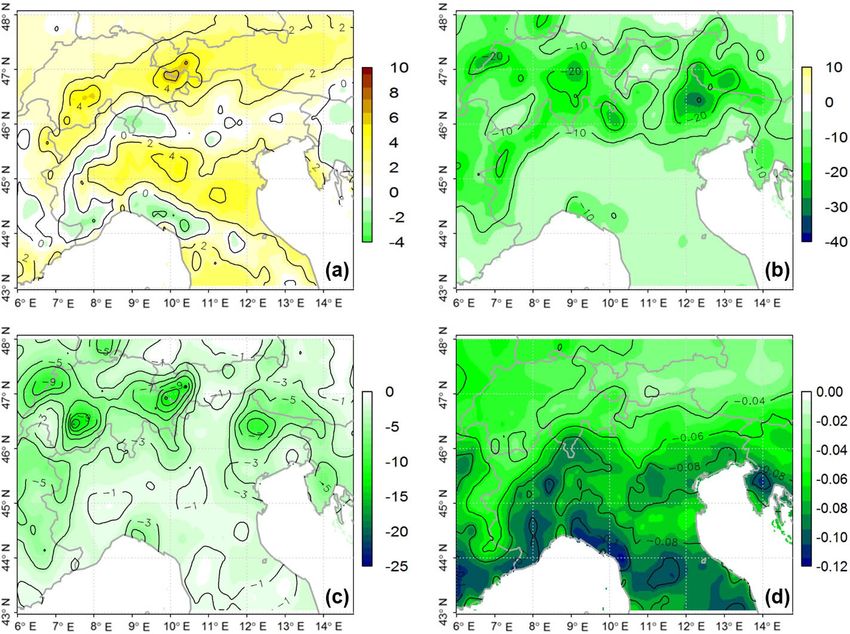
www.hydrol-earth-syst-sci.net/22/3331/2018/ Hydrol. Earth Syst. Sci., 22, 3331–3350, 20183340 C. Cassardo et al.: Climate change over the high-mountain versus plain areas
Variables in Fig. 6 are anomalies of hydrologic budget com- of the soil water, e.g., that used by plants. Here, we limit the
ponents: 1ET, 1PR, 1SR, and 1SM where, e.g., 1ET rep- analysis to the surface SM (i.e., in the top soil layer with a
resents ETFCA2 − ETRC . depth of 5 cm), due to its significant impact on several agri-
Compared to RC, we notice a large increment of NR ev- cultural productions.
erywhere in FCA2 (not shown), with the exception of a few Actually, for the short grass vegetation category consid-
grid points located in the central and western Alps. Regard- ered in our simulations, the root layer is only 5 cm deep, as
ing 1ET (Fig. 6a), plains along the Po River and the northern the grass is only 10 cm high. Despite this value seeming too
off-alpine regions (i.e., middle-slope and/or foot) show the low, it represents the typical height for the landscapes of Po
largest increments, well correlated to 1NR, implying that Valley (at least in its portion occupied by natural vegetation).
most of the available energy excess is used for evaporative Furthermore, the upper soil layer represents the greatest ef-
processes. In contrast, in the Apennines and central Alps, fect of the atmosphere–land surface–soil interactions. Given
1ETs are almost null or slightly negative while 1NRs are in- that we are interested in the present versus future hydrologic
significantly positive. 1PR (Fig. 6b) and 1SR (Fig. 6c) show budget components, it is appropriate to focus on the top soil
similar signals, with a general deficit, especially in the east- layer, where the most dynamic interactions with atmosphere
ern and western Alpine areas. In particular, consistent with and land surface occur. More specifically, the water content
Coppola et al. (2016), 1PR depicts a dipolar pattern, espe- of the soil layer that represents the largest variations of mois-
cially in the eastern part of the Italian Alps, with positive ture is subject to direct evaporation; to the transpiration from
values over the Alps and its north and negative values over vegetation roots; to the gravitational drainage to the second
south of the Alps. Surface 1SM (Fig. 6d) shows a general soil layer; to the capillary suck of moisture from the second
reduction, larger in the zones at latitudes lower than 45◦ N, soil layer; and finally to the eventual precipitation, eventual
whereas surface 1ST (not shown) is almost uniformly larger vegetation drainage, and eventual snow runoff.
in the considered domain. As ETs increase (i.e., 1ET > 0), In order to find the absolute thresholds for SM, we have
SMs generally decrease; however, both decrease over some selected two parameters: PWP and the field capacity. PWP is
regions where 1SMs are strongly negative – on the west- the SM level below which the osmotic pressure of the plant
ern mountainous Emilia-Romagna region and Tuscany, and roots is insufficient to extract water from the soil, and is usu-
along the Po River and in central and southern Piedmont ally considered as an indicator of a serious water deficit for
as well (cf. Fig. 6a and d). When SM decreases below the agricultural practices. The field capacity represents the SM
wilting point, evaporation generally ceases because there is level above which the gravitational drainage, due to soil hy-
no available water for further ET, and the ET anomaly (i.e., draulic conductivity, causes a rapid removal of the excess
1ET) can be negative. Considering that most of those areas water through percolation into deeper layers; thus, it is con-
are important for agricultural production (see, e.g., Prino et sidered to be a threshold above which soil is very wet, as
al., 2009, a study on grapevine in Piedmont region), our re- in the cases of very intense precipitation, sometimes caus-
sults constitute a threatening challenge for future agricultural ing floods. Since these two values change according to the
productivity. soil type and texture, we define a non-dimensional index, QI ,
It is evident that 1ET and 1PR do not show a linear cor- which is independent from soil type, as follows:
relation (cf. Fig. 6a and b). 1ETs are generally positive, q1 − qwi
whereas 1PRs are distributed around null with some positive QI = , (2)
qfc − qwi
peaks on the Apennines and northwestern Italy and large neg-
ative peaks on some Alpine locations. This disparity brings where q1 is the moisture of the top soil layer, qwi is PWP, and
about and/or enhances the nonlinear interactions among tem- qfc is the field capacity. All the values are expressed as a soil
perature, evaporation, soil moisture, etc. Noting that nonlin- saturation ratio. In this way, the soil wetness is categorized in
earity can develop even with small perturbations (e.g., Park, terms of QI as extremely dry soil for QI ≤ 0, and extremely
1999), our results elucidate that similar investigations can wet soil for QI ≥ 1. In this study, we define the thresholds
only be conducted using models that are able to give a correct for dry soil and wet soil as QI = 0 and QI = 0.8, respec-
estimation of energy and hydrologic processes. tively. Note that it is quite rare to see the cases with QI = 1
because the 3-hourly precipitation data from RegCM3 are in-
4.3 Number of dry and wet days in the future climate terpolated to hourly data by keeping the constant rain rate, to
be used as input for UTOPIA. Therefore, we have arbitrarily
The availability of the SM estimations enables us to eval- defined the threshold for wet soil as QI = 0.8.
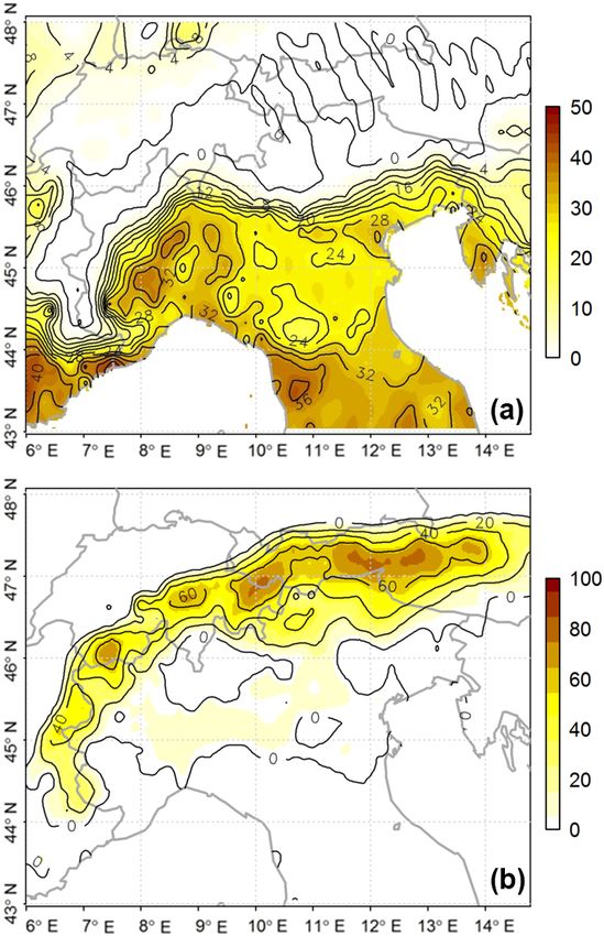
uate the occurrence of dry and wet days, instead of using Figure 7 shows the anomalies of dry and wet days in FCA2 .
atmospheric relative humidity as usual, in a similar way to The number of dry days generally increases in most of the
figure the warm and cold days via the ST estimations. We domain except the Alpine high-mountain areas (Fig. 7a). A
employ SM to assess the dry and wet days in FCs because higher number of dry days (e.g., 30–50 days) occur over the
we consider it to be a more valuable indicator of the soil hy- regions of extreme soil dryness – the coastal areas as well
drologic conditions, directly reflecting the hydrologic status as the off-alpine regions of the Alps and the Apennines (cf.
Hydrol. Earth Syst. Sci., 22, 3331–3350, 2018 www.hydrol-earth-syst-sci.net/22/3331/2018/C. Cassardo et al.: Climate change over the high-mountain versus plain areas 3341
Figure 6. Hydrologic budget components: differences between FCA2 and RC (i.e., FCA2 − RC) of the mean values of (a) ET (in mm), (b) PR
(in mm), (c) SR (in mm), and (d) surface SM (in m3 m−3 ). The mean is calculated over the month of July.
Fig. 6d). The interannual variability of the dry-day occur- and winter (see Figs. 4 and 5). As SM is large over high
rence also decreases (not shown), implying that our results mountains, we have more source of atmospheric moisture
are relatively robust and that we may experience drought over through evaporation there. Then, through the combined ef-
the non-high-mountain areas in almost every year. fect of terrain-induced convective motion, increase in NR
The number of wet days, on the other hand, is almost sta- (though less significant), and pre-existing snow, we can have
tionary over plains but increases by 10–15 days in some lo- more snowmelt (during spring) and more liquid precipitation
calized regions close to the Alps in the Italian side (especially (especially during winter), resulting in more wet days, again
in the Lombardy region), and by even more than 20 days mostly attributed to much a wetter climate in winter.
at the feet of the Alps in Switzerland, France, and Austria
(Fig. 7b). The interannual variability is generally stationary, 4.4 Comparative discussion on previous works
but increases in the areas with the largest numbers of wet
days (not shown). Therefore, in FCA2 , we can have more oc-
The Mediterranean basin is recognized as one of the climatic
casions of reaching high values of surface SM, and hence a
hotspots around the world (Giorgi, 2006; Diffenbaugh and
potentially higher risk of floods. This also implicates a cor-
Giorgi, 2012; Gobiet et al., 2014; Vautard et al., 2014; Paeth
responding higher possibility of hydrogeological instability
et al., 2017). The Alps and their adjacent areas, including the
over the same areas of higher flood risk.
Po River basin in Italy, have been a target region of many
Overall, in the plain areas including the Po Valley, 1ET
climate projection studies, using either a single RCM or an
is positive while 1PR is weakly negative and 1SM is mod-
ensemble of GCMs and/or RCMs (e.g., to mention just a few,
erately negative (especially during summer, as in Figs. 2 and
Gao et al., 2006; Giorgi and Lionello, 2008; Im et al., 2010;
3). With more significant overall increases in NR over plains,
Dobler et al., 2012; Shaltout and Omstedt, 2014; Addor et al.,
the combined effect will bring about larger evaporation and
2014; Coppola et al., 2014, 2016; Gobiet et al., 2014; Torma
lower soil moisture, and thus an overall increase in the num-
et al., 2015; Frei et al., 2018).
ber of dry days, mostly attributed to a much drier climate in
In general, those studies showed good agreements with our
summer. Meanwhile, over the high-mountain areas, PR, SR,
results and produced consistent results of climate projections
and SM increase while ET shows little variation in spring
at the end of 21st century over the study region. However,
www.hydrol-earth-syst-sci.net/22/3331/2018/ Hydrol. Earth Syst. Sci., 22, 3331–3350, 2018You can also read