Economists' erroneous estimates of damages from climate change
←
→
Page content transcription
If your browser does not render page correctly, please read the page content below
Economists’ erroneous
                                                                             estimates of damages from
                                           rspa.royalsocietypublishing.org
                                                                             climate change
                                           Review                            Steve Keen1 , Timothy M. Lenton2 , Antoine
                                                                             Godin3 , Devrim Yilmaz4 , Matheus
                                           Article submitted to journal
                                                                             Grasselli5 , and Timothy J. Garrett6
                                                                             1 University College London, s.keen@isrs.org.uk
                                                                             2 University of Exeter, t.m.lenton@exeter.ac.uk
arXiv:2108.07847v1 [econ.GN] 17 Aug 2021

                                                                             3 Agence Francaise de Developpement, godina@afd.fr
                                                                             4 Agence Francaise de Developpement,

                                                                             yilmazsd@afd.fr
                                                                             5 McMaster University, grasselli@math.mcmaster.ca
                                                                             6 University of Utah, tim.garrett@utah.edu

                                                                              Economists have predicted that damages from
                                                                              global warming will be as low as 2.1% of global
                                                                              economic production for a 3◦ C rise in global
                                                                              average surface temperature, and 7.9% for a 6◦ C
                                                                              rise. Such relatively trivial estimates of economic
                                                                              damages—when these economists otherwise assume
                                                                              that human economic productivity will be an order
                                                                              of magnitude higher than today—contrast strongly
                                                                              with predictions made by scientists of significantly
                                                                              reduced human habitability from climate change.
                                                                              Nonetheless, the coupled economic and climate
                                                                              models used to make such predictions have been
                                                                              influential in the international climate change debate
                                                                              and policy prescriptions. Here we review the
                                                                              empirical work done by economists and show that
                                                                              it severely underestimates damages from climate
                                                                              change by committing several methodological errors,
                                                                              including neglecting tipping points, and assuming
                                                                              that economic sectors not exposed to the weather are
                                                                              insulated from climate change. Most fundamentally,
                                                                              the influential Integrated Assessment Model DICE is
                                                                              shown to be incapable of generating an economic
                                                                              collapse, regardless of the level of damages. Given
                                                                              these flaws, economists’ empirical estimates of
                                                                              economic damages from global warming should be
                                                                              rejected as unscientific, and models that have been
                                                                              calibrated to them, such as DICE, should not be used
                                                                              to evaluate economic risks from climate change, or in
                                                                              the development of policy to attenuate damages.

                                                                              © The Authors. Published by the Royal Society under the terms of the
                                                                              Creative Commons Attribution License http://creativecommons.org/licenses/
                                                                              by/4.0/, which permits unrestricted use, provided the original author and
                                                                              source are credited.
1. Introduction                                                                                                                       2
As a complex global issue, the analysis of climate change requires input from numerous

                                                                                                      rspa.royalsocietypublishing.org Proc R Soc A 0000000
                                                                                                       ..........................................................
intellectual fields. Some economists have contributed by developing what they describe as
“Integrated Assessment Models” (IAMs). IAMs contain components that map economic output
to CO2 generation, CO2 generation to the increase in global average equilibrium temperature,
and the increase in global average equilibrium temperature to the reduction in economic output,
via what they call “damage functions”.
   In this review, we critically evaluate the empirical research done by economists to estimate
these damage functions. We anchor the discussion around the Dynamic Integrated Climate
Economy (DICE) model of W. D. Nordhaus [1], because it was the first model of its kind,
and it has been highly influential in determining climate change policy [2,3]. We also examine
economic damage estimates cited in the Intergovernmental Panel on Climate Change (IPCC) 5th
Assessment Report (AR5) [4], and subsequent estimates [5,6].
   We start in Section 2 with conceptual issues including a serious misrepresentation of the
scientific literature on climate tipping points and a corresponding trivialization of damages that
arises from this misrepresentation. Then in Section 3 we describe a series of methodological
flaws behind these trivial damage estimates, including a discussion of how these obviously
flawed methods became accepted and widely used by economists. In Section 4, we present a self-
contained description of the DICE model and the role that climate damages play in it, including
a discussion of its sensitivity with respect to more severe damages. Section 5 concludes with our
assessment of the contribution of economists to the climate debate and a plea that science-based
approaches should take precedence.

2. Conceptual Issues
(a) Misrepresenting the scientific literature
The existence of tipping points in the Earth’s climate is now an established part of the scientific
literature on climate change [7–11]. The first paper to catalog and attempt to calibrate major
tipping points that could be triggered by global warming reported on a survey of experts,
who considered whether there were large-scale elements of Earth’s climate system that could
be triggered into abrupt and/or irreversible qualitative changes, causing significant qualitative
changes to the climate [7]. These systems were selected subject to the conditions that they
must be “subsystems of the Earth system that are at least subcontinental in scale”, and that
they could be “switched—under certain circumstances—into a qualitatively different state by
small perturbations”. The researchers excluded consideration of “systems in which any threshold
appears inaccessible this century” [7, pp. 1786–87].
    Nine such systems were identified, all but one of which—the Indian Monsoon—could be
tipped by temperature increases alone. The study identified two definite candidates for a tipping
point this century that could be triggered by a rise of between 0.5◦ C and 2◦ C—“Arctic sea-
ice and the Greenland ice sheet”—and noted that “at least five other elements could surprise
us by exhibiting a nearby tipping point” [7, p. 1792] before 2100. A key aspect of subsequent
work [8,9,12] has been the concept of “tipping cascades”, whereby passing a threshold for one
system—say, a temperature above which the Greenland ice sheet irreversibly shrinks—triggers
causal interactions that increase the likelihood that other tipping elements undergo qualitative
transitions—in this example, freshwater input to the North Atlantic increases the risk of a
collapse of the Atlantic Meridional Overturning Circulation (AMOC—also referred to as the
’thermohaline circulation’). Such causal interactions can also be mediated by global temperature
changes whereby tipping one system—e.g. the loss of Arctic summer sea-ice—amplifies global
warming, increasing the likelihood that other other elements undergo a qualitative transition [9].
    The paper [7] concluded that: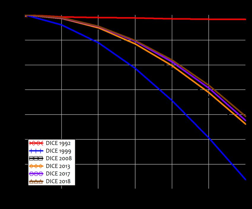
Society may be lulled into a false sense of security by smooth projections of global change.                                            3
      Our synthesis of present knowledge suggests that a variety of tipping elements could reach
      their critical point within this century under anthropogenic climate change. The greatest

                                                                                                              rspa.royalsocietypublishing.org Proc R Soc A 0000000
                                                                                                               ..........................................................
      threats are tipping the Arctic sea-ice and the Greenland ice sheet, and at least five other
      elements could surprise us by exhibiting a nearby tipping point. [7, p. 1792]

   In contrast, the empirical estimates of economic damages from climate change reviewed below
typically assume that climatic tipping points will not be triggered before 2100. One might surmise
that this is because economists have not read this scientific literature, but that is not the case. In
fact, Nordhaus [13] cited [7] to justify not including tipping points in economic damage functions:

      There have been a few systematic surveys of tipping points in earth systems. A particularly
      interesting one by Lenton and colleagues examined the important tipping elements and
      assessed their timing. . . The most important tipping points, in their view, have a threshold
      temperature tipping value of 3◦ C or higher (such as the destruction of the Amazon rain forest)
      or have a time scale of at least 300 years (the Greenland Ice Sheet and the West Antarctic Ice
      Sheet). Their review finds no critical tipping elements with a time horizon less than 300 years until
      global temperatures have increased by at least 3◦ C. [13, p. 60. Emphasis added]

   Nordhaus also referenced [7] in the manual for DICE [1] to justify the use of a simple quadratic
function to relate the increase in global temperature ∆T to the damages to global economic
production D(∆T ):

      The current version assumes that damages are a quadratic function of temperature change
      and does not include sharp thresholds or tipping points, but this is consistent with the survey
      by Lenton et al. (2008). [1, p. 11. Emphasis added]

   The climate damage function is defined as the fraction by which future GDP would be reduced,
relative to what it would be in the complete absence of climate change. In the current version of
DICE, it is quantified as
                                          D(∆T ) = a × ∆T 2 ,                                         (2.1)

where a = 0.00227. Nordhaus observed that this formula predicts “damage of 2.1 percent of
income at 3◦ C, and 7.9 percent of global income at a global temperature rise of 6◦ C” [14, p. 345].
Table 1 contrasts the actual conclusions reached by Lenton et al. with Nordhaus’s claims about
those conclusions in [13] and [1].

   As Lenton later observed:

      There is currently a huge gulf between natural scientists’ understanding of climate tipping
      points and economists’ representations of climate catastrophes in integrated assessment
      models (IAMs). [15, p. 585]

    Nordhaus noted [13, Note 11 to Chapter 5, p. 334)] that his assertion that there are “no critical
tipping elements with a time horizon less than 300 years until global temperatures have increased
by at least 3◦ C” [13, p. 60. Emphasis added] relied in part on a table by Lenton in another
publication, where Lenton constructed what he described as a “simple ‘straw man’ example of
tipping element risk assessment” [16, Table 7.1, p. 185]. This table assessed the 8 tipping elements
on two metrics, “Likelihood of passing a tipping point (by 2100)” and “Relative impact of change
in state (by 3000)”, and gave Arctic summer sea-ice the highest ranking on the first metric, and the
lowest on the second. It is conceivable that this was the basis of Nordhaus’s conclusion that there
were no critical tipping elements this century. However, Lenton explicitly noted that his impact
rating was a relative rating of the eight tipping elements against each other, not an absolute ranking
of their climatic significance:
Table 1. Lenton et al.’s conclusions and their contradictory rendition by Nordhaus 4
rspa.royalsocietypublishing.org Proc R Soc A 0000000
..........................................................
Lenton 2008 “Tipping elements in the Nordhaus 2013 DICE Manual & The Climate
Earth’s climate system” [7] Casino [1,13]
Society may be lulled into a false sense of The current version assumes that damages
security by smooth projections of global are a quadratic function of temperature
change. [7, p.1792] change and does not include sharp
thresholds or tipping points, but this is
consistent with the survey by Lenton et al.
(2008) [1, p. 11]
Our synthesis of present knowledge Their review finds no critical tipping
suggests that a variety of tipping elements elements with a time horizon less than
could reach their critical point within 300 years until global temperatures have
this century under anthropogenic climate increased by at least 3◦ C. [13, p. 60]
change. [7, p.1792]
The greatest threats are tipping the The most important tipping points, in
Arctic sea-ice [0.5–2◦ C warming] and the their view, have a threshold temperature
Greenland ice sheet [1–2◦ C warming], tipping value of 3◦ C or higher (such as the
and at least five other elements could destruction of the Amazon rain forest) . . .
surprise us by exhibiting a nearby tipping [13, p. 60]
point. [7, p.1792 & Table 1, p. 1788]
Arctic . . . summer ice-loss threshold, if not . . . or have a time scale of at least 300
already passed, may be very close and a years (the Greenland Ice Sheet and the West
transition could occur well within this Antarctic Ice Sheet). [13, p. 60]
century. [7, p.1789. Emphasis added]
Impacts are considered in relative terms based on an initial subjective judgment (noting that
most tipping-point impacts, if placed on an absolute scale compared to other climate eventualities,
would be high) [16, p. 186. Emphasis added].
The “transition timescale” column in Lenton’s Table 1 [7, p. 1788] 1 was also an estimate of the
time the complete transition would take from its initial tipping, not the years until a tipping event
would be triggered, as Nordhaus implied. While Lenton et al. did give a timeframe of more than
300 years for the complete melting of the Greenland Ice Sheet (GIS), for example, they noted that
they considered only tipping elements whose fate would be decided this century:
Thus, we focus on the consequences of decisions enacted within this century that trigger a
qualitative change within this millennium, and we exclude tipping elements whose fate is
decided after 2100. [7, p. 1787]
Therefore, contrary to Nordhaus’s assertions, Lenton’s research warned that tipping elements
were likely to be triggered by temperature rises expected this century, and noted that if triggered,
these would have significant impacts upon the climate and biosphere, including its suitability
for human life—and therefore, significant impacts upon the economy. Subsequent research by
Lenton and associates has explicitly criticised the treatment of tipping points by economists in
general (and Nordhaus in particular) [15], calculated that including tipping points in Nordhaus’s
own DICE model can increase the “Social Cost of Carbon” (by which optimal carbon pricing is
calculated) by a factor of greater than eight [8], and proposed 2◦ C as a critical level past which
“tipping cascades” could occur [9,10,15].
1
Table 1 “Policy-relevant potential future tipping elements in the climate system” summarises 15 tipping elements, headed
by the 9 that could tip before 2100.This criticism of economists by scientists has not caused economists in general to recognise 5
tipping points. While some economists have been influenced by Lenton’s work on tipping points
[8,17], subsequent use of the DICE model to inform policy (e.g. setting of the US Federal social
rspa.royalsocietypublishing.org Proc R Soc A 0000000
..........................................................
cost of carbon [2,3]) either ignored tipping points, assigned them such a low probability as
to be irrelevant to damages, or introduced arbitrary discontinuities into damage functions at
temperatures increases well above the 2◦ C level at which the scientific literature indicates that
tipping points become likely [9,10].
One instance of this is Nordhaus’s treatment in DICE of the possibility that the AMOC might
pass a tipping point [18]. While he considers that it could cause a 25% reduction of global GDP
(later increased to 30%), he assigns it probabilities of only 0.6% for a 3◦ C warming scenario in 2090
and 3.4% for a 6◦ C warming scenario in 2175. Nonetheless, given Nordhaus’s other assumptions
in DICE (a rate of risk aversion of 4 and an income elasticity of 0.1), the “willingness to pay” metric
to avoid the AMOC catastrophe is 1% of global GDP for the 3◦ C scenario and 7% for the 6◦ C
scenario. Thus, despite the very low assigned probabilities, this catastrophic risk comprises about
half of total damages estimated by Nordhaus at 3◦ C and the majority of damages at 6◦ C.2 This
indicates that, were this and other tipping points assigned more realistic probabilities, estimated
damages would be much higher. Sure enough, inclusion of tipping point likelihoods in DICE
from the scientific expert elicitation of [12] leads to much higher damages [8].
We now turn to the numerical estimates that economists have made of the economic damages
from climate change.
(b) Trivializing expected damages
The 2014 IPCC Report Climate Change 2014: Impacts, Adaptation, and Vulnerability Part A: Global
and Sectoral Aspects [21] included a chapter on the economic consequence of climate change,
entitled “Key economic sectors and services” [4]. The chapter included a scatter plot with 19
point estimates of temperature increase and global income change [4, Figure 10.1, p. 690]. These
estimates ranged from (+1◦ C, +2.3%)—that is, a 2.3% increase in global income for a 1◦ C increase
in global temperature over pre-industrial levels—to (+5.4◦ C, -6.1%) on the temperature axis, and
(+3.2◦ C, -12.4%) on the income axis, as shown in Figure 1 below.3
These estimates were in comparison to what annual global income would be in the early 22nd
century in the complete absence of global warming, and the chapter noted that “Estimates agree
on the size of the impact (small relative to economic growth)” [4, p. 690]. This is an assertion
that the global economy would only be mildly impacted by global warming—even in the event
of temperature increasing by 5.4◦ C over pre-industrial levels by as soon as 2100 [23]. As the
Executive Summary to that chapter put it:
For most economic sectors, the impact of climate change will be small relative to the impacts
of other drivers (medium evidence, high agreement). Changes in population, age, income,
technology, relative prices, lifestyle, regulation, governance, and many other aspects of
socioeconomic development will have an impact on the supply and demand of economic
goods and services that is large relative to the impact of climate change. [4, p. 662]
Figure 1 also plots the damage function used by Nordhaus in 2018 [14], which was calibrated
against a subset of this data (see [24]). As shown in Table 2 and Figure 2, Nordhaus has used
different functional forms and generally tended to adopt less convex functions with each revision
of the model.
2
Some economists specialising in climate change have argued that the shutdown of AMOC would on balance be economically
beneficial: “The integrated assessment model FUND and a meta-analysis of climate impacts are used to evaluate the change
in human welfare associated with a slowdown of the thermohaline circulation. We find modest, but by and large, positive
effects on human welfare” [19, p. 602]. For scientific assessments of what the shutdown of AMOC would entail, see [19,20].
3
One study, [22], with two methodologies, “Enumeration” and “Statistical”, was cited twice in these estimates. Figure 1
includes damage estimates from [5,6], which were published after [4,21]Figure 1. Adapted from [4, Figure 10.1, p. 690]: Estimates of the total impact of climate change for different values of 6
temperature increase, and damage function from DICE 2016R with 2018 damage coefficient of 0.00227 [14, p. 345]
rspa.royalsocietypublishing.org Proc R Soc A 0000000
..........................................................
Table 2. Nordhaus damage function specifications
Year Function 1 − D(∆T ) Parameters
1√
1992 a [1, p. 85] a = 0.0133 [1, p. 83]
1+ 9 + ∆T
1
1999 1+b×∆T +a×∆T 2
[1, p. 88] b = 0.0045, a = 0.0035 [1, p. 86]
1
2008 1+a×∆T 2
[1, p. 94] a = 0.0028388 [1, p. 91]
1
2013 1+a×∆T 2 [1, p. 100] a = 0.00267 [1, p. 97]
2
2017 1 − a × ∆T [25, p.1] a = 0.00236 [25, p.1]
2018 1 − a × ∆T 2 a = 0.00227 [14, p. 345]
Figure 2 plots these damage functions against temperature increase: with the sole exception of
the change from the initial form in 1992 to a quadratic-based formula, the impact of each change
has been to reduce the predicted damages from climate change.
As mentioned in the previous section, given the scope for fundamental changes to the climate
arising from several tipping points in the Earth’s climate, it is difficult to reconcile the sanguine
conclusion from the estimates in Figure 1, and Nordhaus’s damage function, with the level of
damage to the biosphere expected by climate scientists [8–12,15,26,27].
For simple examples suggesting that economic damages should be much higher, consider
the following. A critical feature of human physiology is our ability to dissipate internal heat
by perspiration. To do so, the external air needs to be colder than our ideal body temperature
of about 37◦ C, and dry enough to absorb our perspiration as well. This becomes impossible
when the combination of heat and humidity, known as the “wet bulb temperature”, exceeds
35◦ C. Above this level, we are unable to dissipate the heat generated by our bodies, and the
accumulated heat will kill a healthy individual within a few hours. Scientists have estimated
that a 3.8◦ C increase in the global average temperature would make Jakarta’s temperature and
humidity combination permanently fatal for humans, while a 5.5◦ C increase would mean thatFigure 2. Nordhaus’s downward revisions to his damage function. 7
rspa.royalsocietypublishing.org Proc R Soc A 0000000
..........................................................
even New York would experience 55 days per year when the combination of temperature and
humidity would be deadly [28, Figure 4, p. 504].
Temperature also affects the viable range for all biological organisms on the planet. Scientists
have estimated that a 4.5◦ C increase in global temperatures would reduce the area of the planet
in which life could exist by 40% or more, with the decline in the livable area of the planet ranging
from a minimum of 30% for mammals to a maximum of 80% for insects [29, Figure 1, p. 792].
It would therefore be tempting for climate scientists to simply outright dismiss the estimates
of damages in Figure 1. Nonetheless, since politicians pay disproportionate attention to the
opinions of economists in formulating most government policies [2,3,30–32],4 this trivialisation
of the dangers of climate change by economists has had serious deleterious effects on the human
response to climate change.
Accordingly, we argue that it is of upmost importance that climate scientists critically engage
with economists on this issue. To this end, in the next section we describe what we consider to be
flawed methods used by economists to arrive at the estimates mentioned above.
3. Methodological Issues
(a) Equating weather and climate
The first numerical estimate made by economists of the impact of climate change on economic
output was generated by Nordhaus in 1991, in the same paper that introduced the cost-benefit
framework for the analysis of climate change [33]. He predicted a 0.25% fall in income for a 3◦ C
increase in global average temperature, while making qualifications to this estimate—which he
4
“it is undeniably the case that economic arguments, claims, and calculations have been the dominant influence on the public
political debate on climate policy in the United States and around the world. . . It is an open question whether the economic
arguments were the cause or only an ex-post justification of the decisions made. . . but there is no doubt that economists have
claimed that their calculations should dictate the proper course of action.” [32, p. 4]described as “ad hoc”—to suggest damages may be 1% of GDP, but were unlikely to be more than 8
2% of GDP:
rspa.royalsocietypublishing.org Proc R Soc A 0000000
..........................................................
damage from a (3◦ C) warming is likely to be around 14 % of national income for United
States in terms of those variables we have been able to quantify. This figure is clearly
incomplete, for it neglects a number of areas that are either inadequately studied or
inherently unquantifiable. We might raise the number to around 1% of total global income
to allow for these unmeasured and unquantifiable factors, although such an adjustment is
purely ad hoc. It is not possible to give precise error bounds around this figure, but my
hunch is that the overall impact upon human activity is unlikely to be larger than 2% of
total output. . . [33, p. 933]
This paper was not used in the IPCC 2014 Report.5 However, its method of estimating damages
from climate change—later described as “Enumeration” by Tol [34]—was replicated by 11 of the
18 studies [18,22,36–44] cited by the IPCC Report [4]. A key element of this method was the
assumption, made without any explanation beyond what is quoted below, that only activities directly
exposed to the weather would be affected by climate change:
Table 5 shows a sectoral breakdown of United States national income, where the economy
is subdivided by the sectoral sensitivity to greenhouse warming. The most sensitive
sectors are likely to be those, such as agriculture and forestry, in which output depends
in a significant way upon climatic variables. At the other extreme are activities, such
as cardiovascular surgery or microprocessor fabrication in ’clean rooms’, which are
undertaken in carefully controlled environments that will not be directly affected by climate
change. Our estimate is that approximately 3% of United States national output is produced
in highly sensitive sectors, another 10% in moderately sensitive sectors, and about 87% in
sectors that are negligibly affected by climate change. [33, p. 930. Emphasis added]
As this quote indicates, this assumption was used to omit entire sectors of the economy from
consideration—including manufacturing, which represented 26% of US GDP in 1991, retail and
wholesale trade (28%), and government (14%)—see Table 3.
Table 3. Extract from Nordhaus’s breakdown of economic activity by vulnerability to climatic change in the US [33, Table
5, p. 931]
“Negligible Effect” Sectors Percentage of total economy
Manufacturing and mining 26.0
Other transportation and communication 5.5
Finance, insurance, and balance real estate 11.4
Trade and other services 27.9
Government services 14.0
Rest of world 2.1
Total “negligible effect” 86.9
The only way to make sense of Nordhaus’s assumption is that he equated “affected by
climate change” to “affected by the weather”, since the only unifying feature of the activities
5
Given the history of how these estimates were assembled, this is more likely to be an oversight than any application of quality
control. Richard Tol, one of the two Coordinating Lead Authors of this chapter, has a history of data errors in his published
papers: two revisions were published to his 2009 paper “The Economic Effects of Climate Change” [34], due to errors that
included omitting negative signs from damage estimates: see [35]. This saga is discussed in detail in a post in Statistical
Modeling, Causal Inference and Social Science and 2 subsequent posts. Nordhaus and Moffat noted further uncorrected
errors in 2017 [24].he assumed would be unaffected is that they occur either indoors or underground. Since these 9
sectors, representing 87% of the economy, are not directly affected by the weather, he expressed
an inability to understand how they could be affected by climate change:
rspa.royalsocietypublishing.org Proc R Soc A 0000000
..........................................................
for the bulk of the economy—manufacturing, mining, utilities, finance, trade, and most
service industries—it is difficult to find major direct impacts of the projected climate
changes over the next 50 to 75 years. [33, p. 932]
The same presumption, that only activities that are directly exposed to the weather will be
affected by climate change, was repeated by the economics chapter of the 2014 IPCC Report as a
“Frequently Asked Question”:
FAQ 10.3 | Are other economic sectors vulnerable to climate change too? Economic
activities such as agriculture, forestry, fisheries, and mining are exposed to the weather
and thus vulnerable to climate change. Other economic activities, such as manufacturing
and services, largely take place in controlled environments and are not really exposed to climate
change. [4, p. 688. Emphasis added]
The only change between Nordhaus in 1991 [33] and the IPCC Report in 2014 [4] was that
the IPCC noted that mining was “exposed to the weather”—presumably in recognition of open-
cut mining. However, none of the studies actually considered the impact of the weather on
mining, while the industries surveyed in [18,22,36–44] exclude the same list of industries excluded
from consideration by Nordhaus—see the “Coverage” column in Table 5. Similarly, the IPCC
special report in 2018 on Global Warming of 1.5◦ C [45] section 3.4.9 “Key Economic Sectors and
Services”, lists tourism, energy (focusing on change in energy demand for heating and cooling),
and transportation (focusing primarily on reduced shipping costs thanks to an ice-free Arctic) as
economic sectors affected by global warming, but makes no mention of impacts on manufacturing
or services.
This assumption that only economic activities that are exposed to the weather will be affected
by climate change can be rejected on at least three grounds.
Firstly, some manifestations of climate change—such as increased wildfires6 [46] and floods
[47]—will affect factories and offices at least as much as they affect the output from those factories
and offices.
Secondly, indoor activities will be unable to continue if temperature increases of the scale
contemplated by economists, such as the 6◦ C increase that Nordhaus asserted would reduce GDP
by only 7.9% [14, p. 345], mean that the places in which factories and offices are located become
uninhabitable—see studies such as [28], which find that lethal temperature levels could affect
areas currently home to 74% of the world’s population by 2100 [28, p. 501]. Factories without
workers produce zero output.
Thirdly, climate change—including impacts on biodiversity and resource depletion as well as
global warming—will affect the availability and costs of essential inputs to production from the
environment: manufacturing cannot occur without non-manmade inputs from the environment,
most obviously energy [48], but clearly also agricultural and mineral inputs. Climate-change
induced stress on power grids and agriculture will clearly impact manufacturing and services
[49]. We speculate that Nordhaus may have ignored this obvious point because the Cobb-
Douglas production function (see equation (4.3) below) used in his DICE model (and most
Neoclassical economic models today), ignores environmental inputs to production, and implies
that production can occur with inputs of labour and machinery alone [48].
6
For some recent news coverage, see for example https://apnews.com/8e4e0818146a72c713de625e902f9962.(b) Using spatial variations in the existing climate as a proxy for climate 10
change
rspa.royalsocietypublishing.org Proc R Soc A 0000000
..........................................................
The second most frequent method used to generate the numbers in Figure 1, labelled as the
“statistical” method [22,50–53] by the IPCC, was described as follows by one of the two co-authors
of the economics chapter of the IPCC 2014 Report [4, p. 659], Richard Tol:
It is based on direct estimates of the welfare impacts, using observed variations (across
space within a single country) in prices and expenditures to discern the effect of climate.
Mendelsohn assumes that the observed variation of economic activity with climate over space holds
over time as well; and uses climate models to estimate the future effect of climate change.
Mendelsohn’s estimates are done per sector for selected countries, extrapolated to other
countries, and then added up. [34, p. 32. Emphasis added]
This method, which is illustrated by Figure 3, derives a statistical fit between temperature
today and income today in the USA,7 typically using a simple regression on the coefficient for a
quadratic function of the temperature deviation from the average national temperature. It then
uses the parameter derived from this regression as the predictor of the impact of global warming
on future GDP.
In the illustration shown in Figure 3, the quadratic coefficient is -0.318% of GDP per 1◦ C
squared rise in temperature over pre-industrial levels. While small, this coefficient is nonetheless
larger than that used by Nordhaus in 2018 to produce his prediction that a 6◦ C increase in global
average temperature will result in a decrease of global income by only 7.9% relative to what it
would have been otherwise in the absence of a temperature rise [14, p. 345] —see equation (2.1).8
Assessing future climate damages by relating current temperature and income is quite clearly
problematic. Figure 3 focuses on present and regional variability within the United States alone,
suggesting existence of an optimal climate from which deviations can be related to lower
productivity. However, the fit is weak. Statistically, the fit to temperature explains just 10% of
Gross State Product (GSP) per capita variability, if we assume that all locations are statistically
independent, and less if we allow for interactions between regions through inter-regional trade.
The most reasonable conclusion is that there is effectively no significant relationship between
contemporaneous GDP and temperature.
However, even the weak fit is statistically misplaced as a guide to future climate damages,
because the underlying premise is flawed. The relationship between regional temperature
variations and regional economic output at a given time has, in principle, no bearing on global
increases over time in average surface temperature and global economic activity. Effectively, what
economists have assumed is that the climate-economy relation, for a specific region of Earth
at a specific time, under the condition of a stable level of atmospheric CO2 , maps onto the
climate-economy relation for the world as a whole as CO2 levels rise.
This assumption commits two fundamental errors. First, any current relationship between
GDP and temperature must reflect regional climate resilience that has developed over centuries.
Obviously, the Gross World Product of the planet taken as a whole is an economically isolated
system, since Earth is unable to engage in interplanetary trade. But the same quite clearly does
not apply to regional economies. For example, Alaska and Maryland are two climate extremes
in the United States that have similar GSP per capita, despite their large differences in average
temperature.9 A prominent climate economist inferred on social media that:
7
Later papers have developed global temperature and GDP comparisons, see for example [51].
8
The range of the quadratic in Figure 3 is restricted to the magnitude of temperature changes for which Nordhaus has given
predictions of damages in refereed papers.
9
The GSP data used in Figure 3 is sourced from the Bureau of Economic Analysis SAINC1 Tables. The figures for Alaska and
Maryland in 2020 were $64, 780 and $68, 258 respectively. Temperature data comes from Current Results. See Table 6.Figure 3. Data and quadratic fit on Temperature and Gross State Product per capita 11
rspa.royalsocietypublishing.org Proc R Soc A 0000000
..........................................................
10K is less than the temperature distance between Alaska and Maryland (about equally
rich), or between Iowa and Florida (about equally rich). Climate is not a primary driver of
income.10
Effectively, what is ignored in this argument is the importance of trade. Trade smooths regional
disparities in a manner that is likely to change with the climate. The USA has been agriculturally
prosperous because of at least three historical coincidences: a currently hospitable climate suitable
for growing crops; a past hospitable climate suitable for the establishment of topsoil; and the
development of a single political, social, and economic system for the distribution of agricultural
output across that system. Thus, current regional productivity, and its distribution, depends not
only on current climate but also on centuries to millennia of prior climatic states, and centuries of
political and economic evolution designed around regional exchange.
Therefore, supposing a rapid change in global average temperature that shifts the climate
suitable for growing crops further north, but at a speed that far exceeds the rate at which new
topsoil is created, and in a manner that transgresses political and social boundaries adapted to
agricultural productivity, the impact on GDP can be expected to be significantly greater than that
reflected by the quadratic curve used in DICE and illustrated in Figure 3. Trade may limit the
sensitivity of production to local climate by offering access to economies in other climates, but
not if those economies are also damaged by climate change.
Consider just one key commodity, grain. Neither Florida nor Alaska, lying at either end of
the temperature extremes of the current climate of the USA, would be nearly as economically
productive were it not for being able to access this primary human food source from Iowa. If, on
the other hand, the climate of Iowa starts to approximate that of Florida, and grain production
there fails, it will not be replaced at higher latitudes due to the poorer topsoil. Even with continued
10
See https://twitter.com/RichardTol/status/1140591420144869381?s=20inter-state trade and new patterns of international trade, equivalently high levels of agricultural 12
prosperity would be difficult to sustain [11].
The second, and more fundamental, concern is that the physics of regional climate variability
rspa.royalsocietypublishing.org Proc R Soc A 0000000
..........................................................
differs from global climate variability, so the economic response should also differ. Climate change
can be expected to introduce new climate extremes not currently experienced in any economically
active region. For example, high wet-bulb temperatures that are known to be life-threatening to
mammals (including humans), and that have not previously existed in the Holocene climate, are
expected to develop over large, densely-inhabited areas. As Sherwood and Huber [26] note when
citing two references in this economic literature,
The damages caused by 10◦ C of warming are typically reckoned at 10–30% of world
GDP [18,39], roughly equivalent to a recession to economic conditions of roughly two
decades earlier in time. While undesirable, this is hardly on par with a likely near-halving
of habitable land, indicating that current assessments are underestimating the seriousness
of climate change. [26, p. 9555]
Further, through tipping elements, the qualitative characteristics of global climate could
change profoundly, including its spatial patterns and modes of temporal variability [15,54]. If the
spatial-temporal pattern of climate variability changes with the mean state, this future challenges
any drawing of inferences from the current spatial-temporal pattern. For example, a possible
shutdown of the AMOC would have global impacts, including threats to monsoons in West
Africa and India as well as to the equability of Western Europe’s climate. In addition, sea level
rise this century could expose hundreds of millions of people to flooding [47] particularly in
the tropics [55]. None of these key aspects can be mathematically characterized by a simple fit
(quadractic or otherwise) of current temperature to current income.
When global warming changes the mean climate state, some regional climates are eliminated
while new climates are introduced, shifting the distribution of regional climates across the face
of the Earth. Of course, not all climate shifts would be regionally detrimental [22], but overall a
mismatch would develop between the new global climate and the conditions under which human
populations developed [11]. In a changing world, potentially billions will be presented with the
option to stay put and try to adapt, or to migrate to more climatologically favorable regions [11].
These geopolitical and economic challenges lie well beyond the narrow economic considerations
demonstrated by the equilibrium quadratic fit of Figure 3.
As a final remark about using spatial variations to estimate damages from climate change, we
notice that the (3.2◦ C,-12.4%) point on Figure 1, taken from [50], appears to be a significant outlier
from the other numbers. However, it was based on the same assumption that geographic data
could serve as a proxy for climate change:
The approach that we will go on to describe in more detail deals exclusively with non-
market impacts whilst making use of spatial variations in the existing climate as an analogue for
climate change. [50, p. 2438. Emphasis added]
The fact that this appears to imply a possible “tipping point” of impacts at 3.2◦ C is thus
coincidental. 11
(c) Computable General Equilibrium Models
Nordhaus’s DICE model is based on the Neoclassical growth model first developed by Ramsey
[56], in which a single individual, treated as a “representative agent” for all of society, maximizes
its utility over an infinite time horizon, by producing and consuming a single commodity (see
Section 4 below). This modelling approach dominates economics today, largely supplanting
an earlier approach called “Computable General Equilibrium” (CGE), in which production of
11
The same observation applies to the post-IPCC 2014 estimate by Burke [5], which we discuss in section (g).multiple commodities using commodities as inputs was modelled using input-output matrices. 13
CGE models were the third most common technique to generate estimates of GDP reduction
due to temperature change from global warming, with two references [23,38] producing three
rspa.royalsocietypublishing.org Proc R Soc A 0000000
..........................................................
estimates.
While CGE models have the strength of including the dependence of the production of
commodities on myriad inputs, including other commodities [57] and inputs from the natural
environment, their reliance upon convergence to equilibrium prices and quantities ignores the
instability of input-output matrices, which are unstable in either prices or quantities, given the
“dual stability theorem” [58, pp. 132-146] (a consequence of the Perron-Frobenius theorem). See
also [32] for the weaknesses of disaggregated economic models as applied to climate change.
However, for the purposes of this review, the main weaknesses of the CGE approach are the
characteristics it shares with the other methods criticized here. Both papers cited by the IPCC
focus upon the same weather-exposed economic sectors (see the “Coverage” column for [23,38]),
and ignore the existence of tipping points.
The economic damage assessments from the General Equilibrium models cited here thus share
the “Enumerative approach” assumption that only industries directly exposed to the weather will
be affected by climate change. This can be seen in the list of phenomena and industries to which
these studies have been applied: “sea-level rise, agriculture, health, energy demand, tourism,
forestry, fisheries, extreme events, energy supply. . . ” [38, p. 4]: the manufacturing, services, and
government sectors, which represent the bulk of the economy, are conspicuously absent. On
tipping points, Roson and van der Mensbrugghe note of their own study that “Catastrophic
events and extreme weather are not taken into account” [23, p. 274].
The impact of the CGE methodology is also generally to reduce the already underestimated
economic damages from climate change. The inputs to these models are the “partial equilibrium”
estimates of individual damages – the effect of higher temperatures on land use, agriculture,
mortality, etc., as estimated by the other papers detailed in Table 5. CGE methods then model
an assumed adaptation to a welfare-maximizing equilibrium, which reduces the impact of these
“partial equilibrium” inputs. Consequently, “general equilibrium estimates tend to be lower,
in absolute terms, than the bottom-up, partial equilibrium estimates. The difference is to be
attributed to the effect of market-driven adaptation” [38, p. 20].
(d) Survey of non-experts
The numerical estimate in Figure 1 and Table 5 of a 3.6% fall in GDP for a 3◦ C increase in global
average temperature by 2090, was derived from what the IPCC Report characterised as “expert
elicitation” [59]. This was a survey by Nordhaus of the opinions of 19 individuals—including
Nordhaus himself—on the impact that increases in global average temperature would have on
global economic output. Nordhaus described them as including ten economists, four “other social
scientists”, and five “natural scientists and engineers”, including three climate scientists,12 but
also noted that eight of the economists came from ”other subdisciplines of economics (those
whose principal concerns lie outside environmental economics)” [59, p. 48]. Though they all had
some connection to climate change,13 as Nordhaus details [59, p. 51], they were not experts in the
sense of the more recent expert elicitation on tipping points [7,12]. Nor were they “encouraged to
remain in their area of expertise” [60, p. 10], as evidenced by the remarks on biodiversity made by
one of the economists, which Nordhaus contrasted with the reservations expressed by a scientist:
One economist (4) stated there would be little impact through ecosystems: ”For my answer,
the existence value [of species] is irrelevant—I don’t care about ants except for drugs.”
12
“Stephen Schneider (climatology). Professor of biological science, Stanford University. . . Paul Waggoner (meteorology and
agricultural science). Distinguished scientist at the Connecticut Agricultural Experiment Station. . . Robert White (atmospheric
science and engineering). President, National Academy of Engineering.” [59, p. 51]
13
The weakest connection was for Larry Summers: “As chief economist at the World Bank, he supervised studies and the
writing of World Development Report 1992, which surveyed development and the environment, and interacted with authors
and the writing of background papers on the economic aspects of global warming”. [59, p. 51]Table 4. Summary statistics from Nordhaus’s survey [59] 14
rspa.royalsocietypublishing.org Proc R Soc A 0000000
..........................................................
Average estimates Individual Percentile Ranges
Scenario
(50th percentile)
10th 90th
(small impact) (large impact)
Label ∆T Date Min Max Median Mean Min Max Min Max
A 3◦ C 2090 0.0% -21.0% -1.9% -3.6% 2.0% -10.0% -0.5% -31.3%
B 6◦ C 2175 0.0% -35.0% -4.7% -6.1% 1.0% -10.0% -1.5% -50.0%
C 6◦ C 2090 -0.8% -62.0% -5.5% -10.4% -1.0% -20.0% -3% -100.0%
By contrast, another respondent cautioned that the loss of genetic potential might lower
the income of the tropical regions substantially. This difference of opinion is on the list of
interesting research topics. [59, p. 50]
Nordhaus’s key question asked for a prediction of the effect on future annual GDP in three
temperature scenarios: (A) a 3◦ C rise by 2090, (B) a 6◦ C rise by 2175, and (C) a 6◦ C rise by 2090.
The figure used by the IPCC from this paper was the mean for scenario A, of a 3.6% fall in GDP for
a 3◦ C increase by 2090. But the most interesting features of this paper were the range of responses,
and the disconnect between the opinions of economists and those of the scientists—only 3 of
whom were scientists with a specialisation in climate change, and one of whom refused to answer
this question. This scientist stated in his dissension that:
I marvel that economists are willing to make quantitative estimates of economic
consequences of climate change where the only measures available are estimates of global
surface average increases in temperature. As [one] who has spent his career worrying about
the vagaries of the dynamics of the atmosphere, I marvel that they can translate a single
global number, an extremely poor surrogate for a description of the climatic conditions,
into quantitative estimates of impacts of global economic conditions. [59, p. 51]
Table 4 summarises the answers given by the 18 respondents. Nordhaus noted the extreme
range of views, which had two polar opposites: economists “whose principal concerns lie outside
environmental economics” and scientists, where the latter’s expectations of economic damages
from global warming were 30 times as large as the former’s:
The major impression emerges from this survey is that experts hold vastly different
views about the potential economic impact of climatic change. At one extreme are the
natural scientists, all three of whom have profound concerns about the economic impacts
of greenhouse warming. . . At the other extreme are the other subdisciplines of economics (those
whose principal concerns lie outside environmental economics); these eight respondents see
much less potential for the calamitous outcome . . . about one-30th of the magnitude estimated
by the natural scientists. [59, p. 48. Emphasis added]
However, this acknowledgement was accompanied by summaries that buried this divergence
in views between the climate change scientists and economists:
The second impression. . . is that for most respondents the best guess of the impact of a 3-
degree warming by 2090, in the words of respondent 17, would be ”small potatoes”. Only
three respondents14 expect the impact of scenario A to be more than 3 percent of GWP.
In terms of economic growth, the median estimated impact for scenario A over the next
14
We deduce, from the previous quote, that these three respondents were the three climate scientists surveyed.century would reduce the growth of per capita incomes from, say, 1.50 percent per year 15
to 1.485 percent per year. One respondent summarized the relaxed view: ”I am impressed
with the view that it takes a very sharp pencil to see the difference between the world with and
rspa.royalsocietypublishing.org Proc R Soc A 0000000
..........................................................
without climate change or with and without mitigation”. [59, p. 48. Emphasis added]
Despite Nordhaus’s comment that “This difference of opinion [between scientists and
economists] is on the list of interesting research topics” [59, p. 50], this difference was not
explored by any researcher in this tradition in the subsequent quarter century. A later, non-
refereed literature survey on the economic impact of climate change by Nordhaus and Moffat,
considered the opinions of economists only, via the economics citation database EconLit [24, pp.
8-10]—see [61, p. 10] for further details.
(e) Shared data
“Integrated Assessment Models” (IAMs) are used by the IPCC and policy makers to generate
predictions of economic damages from climate change that then inform policy formation. Füssel
[62, Table 1, pp. 291-92] lists 18 separate models, and notes the dependencies between them. Of
these 18, 7 are either versions of Nordhaus’s DICE, or based upon it. DICE and two other models,
FUND and PAGE, were used by the USA’s Interagency Working Group on Social Cost of Greenhouse
Gases [2,3] to calculate the US government’s estimate of the “social cost of carbon”. These three
models are calibrated on all or subsets of the numerical estimate papers outlined above. To the
extent to which these models are calibrated on the flawed data points detailed here, they should
not be used to assess the economic implications of climate change.
(f) Epistemological differences and the refereeing process
A vital issue in this literature is how did the refereeing process lead to the publication of
papers which simply assumed that activities which were not directly exposed to the weather
were immune from climate change, and that today’s temperature and income data could be
used as a proxy for the impact of global warming on the economy? The answer may lie in a
methodological principle first espoused by the influential economist Milton Friedman [63], which
rejected the feasibility of assessing a model on the basis of its assumptions. Given the widespread
acceptance of this belief by economists,15 and its incompatibility with the approach to evaluating
assumptions in sciences, it is worth quoting Friedman at length:
In so far as a theory can be said to have “assumptions” at all, and in so far as their
“realism” can be judged independently of the validity of predictions, the relation between
the significance of a theory and the “realism” of its “assumptions” is almost the opposite
of that suggested by the view under criticism. Truly important and significant hypotheses
will be found to have “assumptions” that are wildly inaccurate descriptive representations
of reality, and, in general, the more significant the theory, the more unrealistic the assumptions
(in this sense). The reason is simple. A hypothesis is important if it “explains” much by
little, that is, if it abstracts the common and crucial elements from the mass of complex
and detailed circumstances surrounding the phenomena to be explained and permits valid
predictions on the basis of them alone. To be important, therefore, a hypothesis must be
descriptively false in its assumptions; it takes account of, and accounts for, none of the
many other attendant circumstances, since its very success shows them to be irrelevant for
the phenomena to be explained. To put this point less paradoxically, the relevant question
to ask about the “assumptions” of a theory is not whether they are descriptively “realistic,”
for they never are, but whether they are sufficiently good approximations for the purpose in
hand. And this question can be answered only by seeing whether the theory works, which
means whether it yields sufficiently accurate predictions. The two supposedly independent
tests thus reduce to one test. [63, p. 153. Emphasis added]
15
It is, however, strongly rejected by the minority of non-Neoclassical economists, see for example [64, Chapter 8].This approach has been strongly criticised [65–68], most cogently by the philosopher 16
Musgrave [65] , who classified assumptions into three classes—simplifying, domain and heuristic.
Simplifying assumptions assert that some factor—for example, air resistance in Galileo’s
rspa.royalsocietypublishing.org Proc R Soc A 0000000
..........................................................
demonstration that two dense bodies of different weights fall at the same rate—can be neglected
without significantly affecting the predictions of the theory. Domain assumptions, however,
determine the range of applicability of the theory, so that if the assumption was false, then so
was the model: “The more unrealistic domain assumptions are, the less testable and hence less significant
is the theory” [65, p. 382].
Clearly, the assumptions that 87% of industry will be unaffected by climate change because it
happens in “controlled environments” [4,33, p. 930,p. 688], and that “the observed variation of
economic activity with climate over space holds over time as well” [34, p. 32] are not simplifying
assumptions, because if they are false—which they manifestly are—then the conclusions derived
from them are also false. However, Neoclassical economists have ignored these critiques of
Friedman’s methodology, which is still widely accepted and taught in economics textbooks [69,
pp. 22-24]. Referees trained in the Neoclassical tradition, who would have reviewed Nordhaus’s
1991 paper, would conceivably have treated this assumption as a “simplifying assumption” that
was unchallengeable on methodological grounds.
Given the publication of this paper and several previous papers on climate-related issues
[70–77], Nordhaus himself would have frequently been called upon to referee subsequent
papers on the economics of global warming. Given the tiny number of papers published in
economics journals on climate change—Nicholas Stern observed in 2019 that “the Quarterly
Journal of Economics, which is currently the most-cited journal in the field of economics, has
never published an article on climate change”, while the top 9 general economics journals have
published 57 papers on climate change, out of a total of over 77,000 papers [78]—this has caused
a large degree of conformity in those called upon to referee economic papers on climate change.
Richard Tol observed that the researchers in this field are tightly connected: “Nordhaus and
Mendelsohn are colleagues and collaborators at Yale University; at University College of London,
Fankhauser, Maddison, and I all worked with David Pearce and one another, while Rehdanz was
a student of Maddison and mine” [34, p. 31]. A refereeing process calling upon such a limited
pool of researchers as referees could, as Tol also observed, lead to herding behaviour, rather than
critical evaluation, which would affect the refereeing process as well as the research itself:
it is quite possible that the estimates are not independent, as there are only a relatively small
number of studies, based on similar data, by authors who know each other well. . . although
the number of researchers who published marginal damage cost estimates is larger than
the number of researchers who published total impact estimates, it is still a reasonably
small and close-knit community who may be subject to group-think, peer pressure, and
self-censoring. [34, pp. 37, 42-43]
(g) Post-IPCC 2014 Numerical studies
Studies done since the publication of the IPCC 2014 Report have produced larger estimates of the
economic damages from climate change, using methodologies that differ slightly from the studies
used by the IPCC. Three post-2014 papers [5,6,79] acknowledge the fallacy of using geographic
temperature and income data as a proxy for the impact of global warming on income. The latest
as-yet-unrefereed such study notes that:
Firstly, the literature relies primarily on the cross-sectional approach (see, for instance, Sachs
and Warner 1997, Gallup et al. 1999, Nordhaus 2006, and Dell et al. 2009), and as such
does not take into account the time dimension of the data (i.e., assumes that the observed
relationship across countries holds over time as well). [6, p. 2]You can also read