OceanSODA-ETHZ: a global gridded data set of the surface ocean carbonate system for seasonal to decadal studies of ocean acidification - ESSD
←
→
Page content transcription
If your browser does not render page correctly, please read the page content below
Earth Syst. Sci. Data, 13, 777–808, 2021
https://doi.org/10.5194/essd-13-777-2021
© Author(s) 2021. This work is distributed under
the Creative Commons Attribution 4.0 License.
OceanSODA-ETHZ: a global gridded data set of the
surface ocean carbonate system for seasonal to decadal
studies of ocean acidification
Luke Gregor and Nicolas Gruber
Environmental Physics, Institute of Biogeochemistry and Pollutant Dynamics,
ETH Zurich, 8092 Zurich, Switzerland
Correspondence: Luke Gregor (luke.gregor@usys.ethz.ch)
Received: 4 October 2020 – Discussion started: 22 October 2020
Revised: 8 January 2021 – Accepted: 11 January 2021 – Published: 2 March 2021
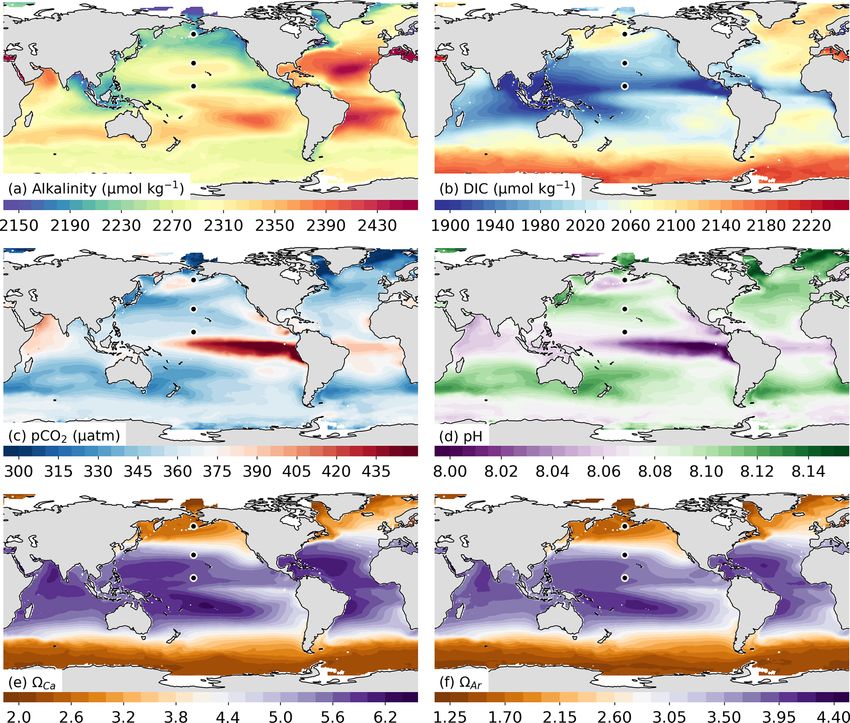
Abstract. Ocean acidification has profoundly altered the ocean’s carbonate chemistry since preindustrial times,
with potentially serious consequences for marine life. Yet, no long-term, global observation-based data set ex-
ists that allows us to study changes in ocean acidification for all carbonate system parameters over the last few
decades. Here, we fill this gap and present a methodologically consistent global data set of all relevant sur-
face ocean parameters, i.e., dissolved inorganic carbon (DIC), total alkalinity (TA), partial pressure of CO2
(pCO2 ), pH, and the saturation state with respect to mineral CaCO3 () at a monthly resolution over the
period 1985 through 2018 at a spatial resolution of 1◦ × 1◦ . This data set, named OceanSODA-ETHZ, was
created by extrapolating in time and space the surface ocean observations of pCO2 (from the Surface Ocean
CO2 Atlas, SOCAT) and total alkalinity (TA; from the Global Ocean Data Analysis Project, GLODAP) using
the newly developed Geospatial Random Cluster Ensemble Regression (GRaCER) method (code available at
https://doi.org/10.5281/zenodo.4455354, Gregor, 2021). This method is based on a two-step (cluster-regression)
approach but extends it by considering an ensemble of such cluster regressions, leading to improved robustness.
Surface ocean DIC, pH, and were then computed from the globally mapped pCO2 and TA using the thermo-
dynamic equations of the carbonate system. For the open ocean, the cluster-regression method estimates pCO2
and TA with global near-zero biases and root mean squared errors of 12 µatm and 13 µmol kg−1 , respectively.
Taking into account also the measurement and representation errors, the total uncertainty increases to 14 µatm
and 21 µmol kg−1 , respectively. We assess the fidelity of the computed parameters by comparing them to di-
rect observations from GLODAP, finding surface ocean pH and DIC global biases of near zero, as well as root
mean squared errors of 0.023 and 16 µmol kg−1 , respectively. These uncertainties are very comparable to those
expected by propagating the total uncertainty from pCO2 and TA through the thermodynamic computations, in-
dicating a robust and conservative assessment of the uncertainties. We illustrate the potential of this new data set
by analyzing the climatological mean seasonal cycles of the different parameters of the surface ocean carbonate
system, highlighting their commonalities and differences. Further, this data set provides a novel constraint on the
global- and basin-scale trends in ocean acidification for all parameters. Concretely, we find for the period 1990
through 2018 global mean trends of 8.6 ± 0.1 µmol kg−1 per decade for DIC, −0.016 ± 0.000 per decade for pH,
16.5 ± 0.1 µatm per decade for pCO2 , and −0.07 ± 0.00 per decade for . The OceanSODA-ETHZ data can be
downloaded from https://doi.org/10.25921/m5wx-ja34 (Gregor and Gruber, 2020).
Published by Copernicus Publications.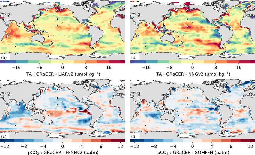
778                                                                 L. Gregor and N. Gruber: Surface ocean acidification data set

1   Introduction                                                       surface ocean pCO2 (e.g., Landschützer et al., 2013, 2016;
                                                                       Rödenbeck et al., 2014; Denvil-Sommer et al., 2019; Gre-
The oceans have taken up roughly one-quarter of the anthro-            gor et al., 2019) and the effort of Lauvset et al. (2015) and
pogenic CO2 that has been released into the atmosphere since           Turk et al. (2017) to analyze long-term trends in pH and
the start of the industrial era (Sabine et al., 2004; Gruber            respectively. But these studies remained limited to one
et al., 2019), modulating the increase in atmospheric CO2              single parameter. At the local-to-regional scale, a number
substantially. However, this buffering of anthropogenic cli-           of long-term time series have provided excellent insights
mate change by the ocean comes with a substantial cost, i.e.,          into the processes and trends of ocean acidification across
ocean acidification (Doney et al., 2009). The uptake of an-            all carbonate system parameters (e.g., Bates et al., 2014),
thropogenic CO2 over the last 150 years has made the sur-              but no global comprehensive view of the historical devel-
face ocean more acidic with a decrease in global mean pH               opment of ocean acidification based on observations exists.
from ∼ 8.2 around 1850 to ∼ 8.1 today (Feely et al., 2009;             This is largely a consequence of the limited observations, al-
Jiang et al., 2019). This decrease in pH equates to a ∼ 30 %           though observational efforts have increased substantially in
increase in the concentration of H+ ions. Some of the an-              the recent decades through efforts such as GOA-ON (Global
thropogenic CO2 taken up from the atmosphere remains in                Ocean Acidification Observing Network, Tilbrook et al.,
the seawater as dissolved CO2 , thus increasing its partial            2019). The OceanSODA (Satellite Oceanographic Datasets
pressure (pCO2 ). In fact, surface ocean pCO2 tends to track           for Acidification) project (https://esa-oceansoda.org, last ac-
the increase in atmospheric pCO2 rather closely (e.g., Bates           cess: 12 September 2020), which this study forms part of,
et al., 2014) owing to the ∼ 1-year timescale for the equili-          aims to close this gap by linking satellite observations with
bration of CO2 across the air–sea interface (Sarmiento and             in situ observations of the marine carbonate system.
Gruber, 2006), which is smaller than the decadal timescale                In line with the goal of the OceanSODA project, we aim to
increase in atmospheric CO2 (Friedlingstein et al., 2019).             develop a global, observation-based data set documenting the
While some of the added CO2 stays as CO2 , the majority                progression of ocean acidification over the recent decades.
of it is titrated away by the ocean’s carbonate ion (Sarmiento         Such a data set will be crucial to put the current trends of
and Gruber, 2006), leading to a substantial reduction in its           ocean acidification into the context of the changes over the
concentration. This reduces the saturation state () with re-          last few decades. By also describing the level of variability
gard to the mineral calcium carbonate (CaCO3 ), where an              in ocean acidification around the long-term trend, it will also
of < 1 leads to dissolution of CaCO3 .                                 help to better understand the challenges that marine organ-
   These chemical changes, collectively described as ocean             isms are facing. Additionally, it will permit us to explore in
acidification, will have a profound impact on marine organ-            much more detail how ocean acidification has unfolded re-
isms, especially those that form shells made of CaCO3 (Orr             gionally and potentially deviated from the simple model of it
et al., 2005; Fabry et al., 2008; Doney et al., 2009; Bed-             being dependent on the rise in atmospheric CO2 .
naršek et al., 2019; Doney et al., 2020). Calcifying organ-               The well-measurable parameters of the marine carbonate
isms living in high latitudes and subtropical and tropical up-         system are dissolved inorganic carbon (DIC), total alkalinity
welling regions, with their naturally low  and pH, may be             (TA), pH, and the partial pressure of carbon dioxide (pCO2 ).
particularly vulnerable, as these regions will be among the            Very few measurement programs measure all of these param-
first to cross critical saturation thresholds (Orr et al., 2005;       eters concurrently. In fact, the vast majority of the observa-
Steinacher et al., 2009; Gruber et al., 2012; Franco et al.,           tional programs measure only one parameter, with pCO2 be-
2018; Fabry et al., 2009; Hauri et al., 2016; Negrete-García           ing the most often measured one, followed by DIC, TA, and
et al., 2019). However, marine organisms may be susceptible            pH (Bakker et al., 2016; Olsen et al., 2019). Since two pa-
to changes even where  > 1 due to a shift in energetic re-            rameters are sufficient to fully describe the marine carbon-
quirements for shell formation (Orr et al., 2005; Pörtner and          ate system, any combination of two will permit us to fully
Farrell, 2008). For example, it is well known that corals start        reconstruct the entire carbonate system. But not all combi-
to decrease their calcification already at saturation states well      nation are equally suited, given the uncertainties in the mea-
above 3 (Gattuso et al., 1998). Ocean acidification will thus          surements, the uncertainties in the coefficients of the carbon-
have a significant economic impact on fisheries and tourism            ate chemistry, and the spatiotemporal coverage vis-à-vis the
through the impact on shellfish and corals, respectively (Coo-         variability of these parameters.
ley and Doney, 2009; Doney et al., 2020).                                 We use here the pair pCO2 and TA as the basis for our
   At the global scale, most of what we know about the                 reconstruction for two reasons. First, these are the best ob-
progression of ocean acidification in the recent decades has           served parameters relative to their spatiotemporal variabil-
come from either models (Bopp et al., 2013; Kwiatkowski                ity, permitting us to develop better predictive models for the
et al., 2020) or from the combination of model-based trends            global surface ocean than possible for, e.g., DIC and pH. Sec-
with observation-based climatologies (Feely et al., 2009;              ond, detailed assessments of the internal consistency of the
Jiang et al., 2019). A notable exception is the large num-             oceanic carbonate system have shown that pCO2 and TA are
ber of studies that have analyzed the trends and variability of        a well-suited pair to estimate pH, owing to the reliability of

Earth Syst. Sci. Data, 13, 777–808, 2021                                                https://doi.org/10.5194/essd-13-777-2021
L. Gregor and N. Gruber: Surface ocean acidification data set                                                                 779

the measurements and the predictive accuracy (Bockmon and         regression and tree-based regression, have also been used
Dickson, 2015; Bakker et al., 2016; Raimondi et al., 2019).       with similar success (Rödenbeck et al., 2014; Gregor et al.,
This is not the case if DIC was used instead of TA. Our choice    2019). However, the specific implementation of the methods
is supported by Takahashi et al. (2014), who developed the        is what sets the assortment of methods apart. For example,
first seasonal climatology of all surface ocean carbonate sys-    the SOM-FFN method of Landschützer et al. (2013) and the
tem parameters using the same pair.                               CSIR-ML6 method of Gregor et al. (2019) (among others)
   Measurements of pCO2 are abundant compared to the              first cluster the data based on a certain set of climatological
other variables, due to a well-established and robust under-      predictors and then perform a regression on pCO2 for each
way sampling protocol that allows instruments to also be          resulting cluster. An alternate approach, used by both the
installed on non-scientific vessels under the Voluntary Ob-       CMEMS-FFNNv2 (Denvil-Sommer et al., 2019) and NIES-
serving Ship (VOS) program (Bakker et al., 2016; Pierrot          FNN (Zeng et al., 2014) methods, is to include the positional
et al., 2009). High-quality pCO2 data are also easily acces-      coordinates, without the need for subsetting the data by clus-
sible thanks to the Surface Ocean CO2 Atlas (SOCAT) that          tering. Despite the differences in implementation and regres-
consolidates underway pCO2 observations and ensures the           sion algorithms, the majority of methods achieve for the open
quality of observations (Bakker et al., 2016). Total alkalinity   ocean a root mean squared error (RMSE) of roughly 18 µatm
is not as widely measured as pCO2 due to the fact that mea-       when compared with SOCAT (Gregor et al., 2019). However,
surements are made discretely with bottle samples (Dickson        each of these methods has its strengths and weaknesses; for
et al., 2007). But, fortunately, TA is highly correlated with     example, the SOM-FFN and CSIR-ML6 methods are able
salinity on a global scale (r = 0.96), making it a suitable       to generalize estimates in data-sparse regions due to infor-
variable for prediction with a < 10 % error of the observed       mation sharing within a cluster, but the methods suffer from
range (Lee et al., 2006; Olsen et al., 2019; Broullón et al.,     discrete boundaries where clusters meet (Gregor et al., 2019).
2018). Further, the accessibility of TA measurements is made      These discrete boundaries may introduce artifacts when ap-
possible through the continued efforts of the Global Ocean        plied to certain questions. This is also the case, for example,
Data Analysis Project (GLODAP; Olsen et al., 2019). We            in the blended open-ocean–coastal-ocean product of Land-
discarded the option to use DIC instead of TA, even though        schützer et al. (2020), where the authors combined the open-
DIC is slightly more often sampled than TA. This decision is      ocean estimate of Landschützer et al. (2016) with the coastal
based on the fact that DIC is more variable than TA, and also     product of Laruelle et al. (2017).
its correlation with salinity is much lower. As a result, it is      The extrapolation of TA onto a global grid is also well
difficult to develop predictive models for DIC that are as ac-    established (Gruber et al., 1996; Millero et al., 1998; Lee
curate and precise as those for TA. Oceanic pH is also not an     et al., 2006; Takahashi et al., 2014; Good et al., 2013;
option, since historically it has been measured far less often    Carton et al., 2018; Bittig et al., 2018). The highly lin-
than the other parameters. This is changing, since progress       ear relationship between salinity and TA means that lin-
with reference materials and new sensors have permitted a         ear regressions have been able for quite some time to esti-
tremendous increase in the number of pH measurements in           mate TA with adequate accuracy. For example, Gruber et al.
recent years, largely benefiting from deployments of biogeo-      (1996) developed a globally applicable multi-linear regres-
chemical Argo floats (Claustre et al., 2020).                     sion (MLR) model involving salinity and the conservative
   The actual spatial and temporal coverage for any of these      tracer PO (PO = O2 + 170 · PO4 , Broecker and Peng, 1974)
parameters is very low. Even for pCO2 , i.e., the parameter       and achieved a global RMSE of 11 µmol kg−1 . Lee et al.
with the densest coverage, only about 1.4 % of the global sur-    (2006) also used a MLR approach but differentiated it re-
face ocean has been sampled in any given month over the past      gionally using salinity, temperature, and spatial coordinates
30 years (Bakker et al., 2016). Thus, the global-scale recon-     as independent variables. The same approach was followed
struction of the progression of ocean acidification requires      by Takahashi et al. (1993). More recently, more nuanced
a very substantial interpolation and extrapolation effort. Ad-    and non-linear regression approaches have improved upon
vances in remote sensing (Land et al., 2019), and the increas-    the MLR approaches (Sasse et al., 2013; Carter et al., 2018;
ing power and usability of machine learning techniques, have      Broullón et al., 2018; Bittig et al., 2018). For example, the lo-
permitted us to address this challenge, leading to a prolifera-   cally interpolated alkalinity regression (LIARv2) still makes
tion of such efforts. However, they vary greatly between the      use of linear regression but interpolates the regression coef-
different parameters of the marine carbonate system.              ficients spatially from a fixed set of trained regression nodes
   By far the most established efforts are those that interpo-    located at every fifth point (Carter et al., 2016). Sasse et al.
late and extrapolate the ocean pCO2 observations, as demon-       (2013) used a self-organizing map approach coupled with
strated by the intercomparison project by Rödenbeck et al.        a local linear optimizer (called SOMLO) and achieved a
(2015). Feed-forward neural networks (FFNNs) have be-             global RMSE of 9 µmol kg−1 . A similar RMSE was achieved
come one of the favored tools (Landschützer et al., 2013;         by Broullón et al. (2018) using a neural network approach
Zeng et al., 2014; Denvil-Sommer et al., 2019), but other         (NNGv2). These low RMSE levels were also achieved by
statistical and machine learning methods, such as Bayesian        these studies avoiding the nearshore and coastal environ-

https://doi.org/10.5194/essd-13-777-2021                                            Earth Syst. Sci. Data, 13, 777–808, 2021
780                                                                L. Gregor and N. Gruber: Surface ocean acidification data set

ments, where variability in the surface ocean carbonate sys-          (1985 through 2018), we follow the three steps depicted by
tem is much higher than in the open ocean (Laruelle et al.,           the flow diagram in Fig. 1. First, we develop a statistical
2017). In addition to these global regressions, several region-       model for the measured TA and pCO2 using the newly de-
ally specific regressions were developed (see Table 1 in Land         veloped GRaCER method. This method itself consists of two
et al., 2019).                                                        steps, i.e., a cluster step, where the target variables are clus-
   In comparison, very few efforts attempted to interpolate           tered regionally, and a regression step, where for each clus-
and extrapolate DIC. Lee et al. (2000) were the first to pro-         ter a regression is evaluated. These two steps are repeated
duce a global map of DIC using a regression methodology;              multiple times, creating an ensemble of models; second, we
however, their application employed a regional multi-linear           map these two quantities globally and over time using this
regression model similar to that used later to map TA. But            ensemble of statistical models and global observations of the
their application was limited to the generation of a seasonal         predictor variables; third and last, we use a thermodynamic
climatology. It was not until Sasse et al. (2013) when the            model of the seawater carbonate system to compute the re-
first global reconstruction of the temporal progression of            maining parameters of the surface ocean carbonate system,
DIC over multiple years was published. They used the same             namely DIC, pH, and . Along the way, we extensively eval-
SOMLO method as they had used for TA, creating global                 uate and test each step with independent observations. We
maps of DIC with a RMSE of 11 µmol kg−1 . More recently,              refer to the data set with the evaluated and complete marine
Keppler et al. (2020) used the SOM-FFN method of Land-                carbonate system as OceanSODA-ETHZ.
schützer et al. (2013) to reconstruct DIC throughout the up-             Next, we describe the concept of the GRaCER method and
per water column on a monthly basis, but they limited their           then detail its implementation for pCO2 and TA. This is fol-
discussion to the mean seasonal cycle.                                lowed by a description of the numerous types of data em-
   Here, to map TA and pCO2 globally, including the coastal           ployed and how they were prepared. Lastly, we demonstrate
ocean, the Arctic, and the Mediterranean, we use a newly              how we used a thermodynamic model to derive the remaining
developed two-step cluster-regression approach that is simi-          parameters of the marine carbonate system.
lar in design to the SOM-FFN method (Landschützer et al.,
2013, 2016) but extend it by using an ensemble of such clus-          2.1   GRaCER algorithm
ter regressions. This method, referred to as Geospatial Ran-
dom Cluster Ensemble Regression (GRaCER), increases the               The GRaCER algorithm builds conceptually on a series
robustness of the estimates considerably. It also removes the         of cluster-regression algorithms that have been successfully
boundary problems inherent in all methods that use fixed re-          used for the interpolation and extrapolation of surface ocean
gional boundaries. We apply the same methodology to TA                pCO2 (Sasse et al., 2013; Landschützer et al., 2013, 2016;
and pCO2 , resulting in methodologically consistent global            Iida et al., 2015; Gregor et al., 2019). The main advantage of
estimates of the two parameters, from which DIC, pH, and             such a two-step approach is that the first clustering step orga-
can then be computed using the well-established thermody-             nizes the variability regionally and temporally. This greatly
namic models of the seawater carbonate system. These lat-             enhances then the fidelity of the second step, i.e., the regres-
ter estimates can then be compared against the many avail-            sion, as the size of the regression problem is reduced from
able DIC and pH measurements, providing a large set of in-            the global domain to smaller, more homogeneous regions. A
dependent data to assess the fidelity of our estimates. This          second advantage is that this clustering brings together re-
also requires a good understanding of the different sources           gions with similar seasonality and similar co-variability with
of uncertainties – including those emanating from sampling            potential predictors, irrespective of the number of observa-
and measurement, from the statistical modeling, and from the          tions. The regression step explains the variability within each
lack of representativeness, i.e., the fact that a local measure-      region over time and space dimensions, including interan-
ment is not representative for the large pixel (100 × 100 km          nual variability. Further, the clustering permits the regression
and 1 month) – that one models in our regressions.                    to transfer information from spatially distant but geochem-
   The rest of the paper describes the data and methods used          ically similar regions, making the interpolation and extrap-
to calculate this data set for ocean acidification. The uncer-        olation more robust in data-poor regions. The main innova-
tainties of the predictions are assessed, followed by the pre-        tion of the GRaCER algorithm relative to the previously used
sentation of the data with a focus on the seasonal cycle. Last,       two-step approaches is its use of ensembles of cluster regres-
we discuss the implications of the uncertainties for the use of       sions, i.e., the generation of a whole series of clusters and
the derived marine carbonate system.                                  corresponding regressions, which overcomes the boundary
                                                                      problems that are inherent in all two-step approaches.
                                                                         For the clustering step, we use monthly climatological data
2   Methods                                                           of pCO2 and TA and related parameters (Fig. 2a–c) to deter-
                                                                      mine the main patterns of variability of the target variable and
To reconstruct the global progression of all parameters of the        its co-variability with potential predictor variables. We opted
surface ocean carbonate system over the last three decades            for a clustering on climatological data rather than on the ac-

Earth Syst. Sci. Data, 13, 777–808, 2021                                                https://doi.org/10.5194/essd-13-777-2021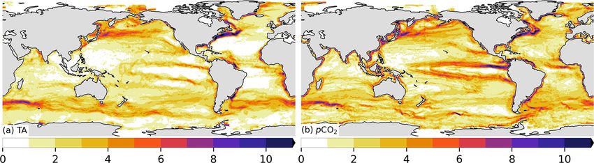
L. Gregor and N. Gruber: Surface ocean acidification data set                                                                              781

Figure 1. Schematic flow diagram showing the three steps required to reconstruct the surface ocean carbonate system. In the first step (yellow
hexagons), the GRaCER (Geospatial Random Cluster Ensemble regression) method is used to develop statistical models for the observed TA
(left) and pCO2 (right) fields. In the second step (orange rectangles), these statistical models are used to extrapolate these two parameters
over time and space using ancillary observations, primarily stemming from satellite observations. In the third step (red oval), the interpolated
and extrapolated TA and pCO2 fields are then used to compute the remaining parameters of the surface ocean carbonate system, namely
DIC, pH, and the saturation state of seawater with regard to mineral CaCO3 , . The output of steps two and three is the OceanSODA-ETHZ
product. Also shown are the various data sets and data flows used in this study. The different lines indicate whether data are used for training
(solid lines), testing (dashed lines), or output with an estimate of uncertainty, where independent test data are shown with gray dashed lines.
The gridded/satellite data are summarized in Table 1. Independent test data are shown by the purple box. pyCO2SYS is the software used to
solve the marine carbonate system and propagate uncertainties (Humphreys et al., 2020).

tual monthly data in order to clearly focus on the clustering             ter suited to capture the smaller level variations associated
step’s role to isolate primarily regions with the same seasonal           with the interannual variability and trends. The mini-batch
cycle. The alternative approach, i.e., to cluster on the monthly          K-means implementation in the Python scikit-learn package
data, is also more prone to errors since the climatological dis-          is used to perform the clustering due to its computational ef-
tributions are better known than their month-to-month vari-               ficiency and scalability with large data sets (Pedregosa et al.,
ations. Finally, clustering on monthly data would also take               2011). A user-defined number of cluster centers are initi-
away signals from the regression step, which is actually bet-             ated, where cluster centers represent the mean of the points

https://doi.org/10.5194/essd-13-777-2021                                                      Earth Syst. Sci. Data, 13, 777–808, 2021
782                                                                   L. Gregor and N. Gruber: Surface ocean acidification data set

Figure 2. A schematic showing the steps used in the GRaCER method for a single month. Panels (a)–(c) show a subset of the clusters of
a single ensemble member (h), with the adjacent scatter plots (d)–(f) showing the training data for each cluster and the linear regression
models for that cluster (with toy data). Panels (g)–(i) show the ensemble member estimates for a subset of three members for pCO2 . Panel (j)
shows the ensemble mean for all ensemble members, which includes ensemble members not shown in panels (g)–(i).

in a cluster. The K-means++ algorithm is used to initiate                2.2     Algorithm implementation
the cluster centers; it randomly selects the location of the
first cluster center and then iteratively selects a best-guess           2.2.1    Total alkalinity
location for the remaining cluster centers. Thereafter, the al-
gorithm minimizes the distance between cluster centers and
                                                                         For the estimation of TA, we employ the support vector
data points in the variable space. Once the clusters have been
                                                                         regression (SVR) method with 12 clusters and 16 ensem-
defined for the climatological domain, the co-located training
                                                                         ble members. The clustering is performed on climatological
data are assigned to the monthly clusters.
                                                                         mean TA, sea-surface salinity (SSS), sea-surface temperature
   The regression is then performed individually for each of
                                                                         (SST), and nitrate (NO−  3 ; Table 1 and Sect. 2.3 below). The
the clusters (Fig. 2d–f). The GRaCER method does not use
                                                                         optimal variables on which clustering should be performed
a prescribed regression method – rather the appropriate algo-
                                                                         were selected by assessing the regression scores of each com-
rithm for the particular use case is implemented. Importantly,
                                                                         bination of variables following the methodology of Gregor
the algorithm must be able to scale appropriately to the size
                                                                         et al. (2019). All data are standardized to the mean (µ) and
of the problem. For example, the training data set for TA is
                                                                         standard deviation (σ ) prior to clustering ( (x−µ)
                                                                                                                         σ ), after which
1/20th of the size of the pCO2 training data set; thus a more
                                                                         TA is given 3 times the weight of the other variables.
computationally expensive method can be used to predict TA.
                                                                            A similar exhaustive search was used for determining the
   The ensemble members are created by performing the
                                                                         number of clusters. The number of ensemble members was
cluster-regression step multiple times. Creating an ensem-
                                                                         chosen by the number above which there is no longer an in-
ble is possible due to the fact that each clustering instance
                                                                         crease in performance, analogous to the number of trees in a
is slightly different (Fig. 2g–i). In practice, the spatial dis-
                                                                         random forest. Test data are a subset of years spaced 3 years
tribution of the clusters is similar; i.e., there is consistency
                                                                         apart starting in 1985. We ensure that the models are not
in the typology of the clusters, particularly in regions where
                                                                         overfitted by selecting hyper-parameters using K-fold cross
clusters are well defined, such as in the subtropical gyres and
                                                                         validation (further details are in Sect. A3).
in the tropical eastern Pacific. However, there are regions that
                                                                            To regress and map TA, we use SSS, SST, silicic acid
belong to different clusters; i.e., there is slight variance in the                                              3−
                                                                         (H4 SiO4 ), and N ∗ = NO−  3 − 16 · PO4 (nitrogen excess rel-
typology between ensemble members. The differences are
                                                                         ative to phosphate in terms of the Redfield N : P ratio sim-
due to the random initialization of the first cluster center in
                                                                         plified from Gruber and Sarmiento, 1997) as predictors. Our
the K-means clustering step and the fact that clustering vari-
                                                                         choice of SSS and SST as predictors is easily justified by
ables for some regions have weak gradients in spatial auto-
                                                                         these two variables accounting for the majority of TA vari-
correlation resulting in weak association with a cluster. In
                                                                         ability (Lee et al., 2006; Carter et al., 2018). The addition
practice, this means that the locations of cluster boundaries
                                                                         of H4 SiO4 and N ∗ as predictors is to account for seasonal
vary between ensemble members; thus the ensemble mean
                                                                         changes in primary production that has an impact on TA
does not have discrete boundaries (Fig. 2j).
                                                                         (Wolf-Gladrow et al., 2007; Carter et al., 2018). Further, N ∗
                                                                         expresses the zonal differences between and within the large
                                                                                                                                 3−
                                                                         ocean basins better than using simply NO−       3 or PO4 – an

Earth Syst. Sci. Data, 13, 777–808, 2021                                                    https://doi.org/10.5194/essd-13-777-2021
L. Gregor and N. Gruber: Surface ocean acidification data set                                                                   783

important consideration, since coordinates (i.e., latitude and       close tracking of oceanic pCO2 to atmospheric CO2 concen-
longitude) are not included in our set of predictors.                trations (Bates et al., 2014).

2.2.2   Partial pressure of CO2                                      2.3     Data

For the estimation of pCO2 , we use two regression methods,          Data are used to develop the two-step GRaCER model, i.e.,
i.e., GBDTs (gradient boosted decision trees) and FFNNv2             clustering and regression, and to evaluate the estimates. Ta-
(feed-forward neural network). These are implemented with            ble 1 provides an overview of all data employed and the pur-
21 clusters and 16 ensemble members (eight each). The num-           poses for which they are used, and Table 2 shows the cor-
ber of clusters is at the upper end of the range compared            responding source of the data. We describe each data set by
with the number of clusters used by the MPI-SOMFFN or                parameter and use.
CSIR-ML6 methods. However, testing has shown that addi-
tional clusters are required to account for the additional com-      2.3.1    Data for clustering
plexity by our inclusion of data from the coastal, Arctic, and
                                                                     For the clustering of TA, we used the mapped product of to-
Mediterranean seas.
                                                                     tal alkalinity (TAmap ) from the GLODAPv2 (Lauvset et al.,
   Clustering is performed on climatological values of pCO2 ,
                                                                     2016). This product represents a quasi-annual mean as it was
SST, mixed-layer depth (MLD), and chlorophyll a, with ad-
                                                                     generated without consideration of the seasonal cycle. We re-
ditional weighting given to pCO2 . As with TA, all variables
                                                                     peat this quasi-annual mean TA to create a monthly data set
are standardized prior to clustering with (x−µ)  σ , after which     over which clustering can be performed. We thus assume that
pCO2 is multiplied by 3 to give it stronger weighting.
                                                                     the spatial variability of TA is larger than the seasonal vari-
   Details of the regression method and of the hyper-
                                                                     ability. This is backed by Takahashi et al. (2014) and Broul-
parameter selection are given in Sect. A3. Test data are se-
                                                                     lón et al. (2018), who found that the seasonal variability of
lected as every fifth year starting in 1985, and validation data
                                                                     TA for the majority of the ocean was more than a factor of
for early stopping are selected using the same approach start-
                                                                     10 smaller than the spatial variability.
ing in 1987, where the latter are used for early stopping to re-
                                                                        For the clustering step of pCO2 , we use four data-based
duce overfitting and keep model complexity within bounds.
                                                                     products resampled and gridded to a monthly by 1◦ × 1◦ res-
   The regression and mapping is performed with the fol-                            map
                                                                     olution (pCO2 ), namely LDEO by Takahashi et al. (2014),
lowing variables as predictors: SST, SSS, the logarithm of
                                                                     MPI-SOMFFN by Landschützer et al. (2016), Jena-MLS by
chlorophyll a, the logarithm of mixed-layer depth, the merid-
                                                                     Rödenbeck et al. (2014), and CMEMS-FFNNv2 by Denvil-
ional and zonal components of the surface winds, the sine
                                                                     Sommer et al. (2019). It may seem tautological to use other
and cosine of day365·180
                    of year·π
                              , and the atmospheric dry-air mixing
                                                                     machine learning estimates, but these data are just used to
ratio (xCO2 ). These predictors are the same as used by Gre-
                                                                     create regional clusters; i.e., they are not used in the regres-
gor et al. (2019), and various combinations of these methods
                                                                     sion step. Relative to previous two-step approaches (Land-
have been used by previous approaches (Landschützer et al.,
                                                                     schützer et al., 2016; Denvil-Sommer et al., 2019), which
2014; Denvil-Sommer et al., 2019).
                                                                     used just the LDEO product, we expanded on this by includ-
   It is important to note that the predictors are proxies for the
                                                                     ing three more estimates. In doing so, we make the implicit
spatiotemporal changes in pCO2 and do not necessarily ex-
                                                                     assumption that this ensemble of estimates is a better repre-
plain the physical mechanism by which changes in pCO2 are
                                                                     sentation of the pCO2 monthly climatology than the LDEO
driven. For example, an increase in sea-surface temperature
                                                                     climatology alone.
in the subtropics results in an increase in pCO2 as shown
                                                                        SSS is from the Simple Ocean Data Assimilation (SODA)
by Takahashi et al. (1993) and Lefèvre and Taylor (2002).
                                                                     analysis (Carton et al., 2018) and SST from the Operational
In contrast, surface warming in the Southern Ocean can be
                                                                     Sea Surface Temperature and Sea Ice Analysis (OSTIA)
a proxy for stratification that reduces outcropping of high-
                                                                     product (Good et al., 2019, 2020). N ∗ is calculated using
CO2 waters (Landschützer et al., 2015; Gregor et al., 2018).                                                     3−
                                                                     monthly climatologies of NO−      3 and PO4 from the World
Similarly, changes in SSS and MLD also capture the dis-
                                                                     Ocean Atlas updated in 2018 (Boyer et al., 2013). We use
tribution and processes that drive changes in surface pCO2 ,
                                                                     the monthly climatology of density-based mixed-layer depth
such as stratification and mixing. However, the climatologi-
                                                                     (MLD) from Holte et al. (2017) that is estimated from Argo
cal MLD product used here does not capture interannual vari-
                                                                     float profiles. The MLD data product merges monthly esti-
ability in stratification and mixing. We thus include the two
                                                                     mates of MLD from multiple years but is averaged into a
surface wind components that, along with SST, are a proxy
                                                                     climatology due to the paucity of data on an annual scale. A
for wind-driven mixing and upwelling. Chlorophyll is also
                                                                     two-dimensional moving average filter is applied to the MLD
an important driver of pCO2 on a local scale, particularly
                                                                     to interpolate missing data and remove the noise introduced
in the high-latitude regions where high primary productivity
                                                                     by interannual and sub-monthly variability.
results in rapid uptake of pCO2 (Bakker et al., 2008; Gre-
gor et al., 2018). Lastly, xCO2 is included to account for the

https://doi.org/10.5194/essd-13-777-2021                                               Earth Syst. Sci. Data, 13, 777–808, 2021
784                                                                      L. Gregor and N. Gruber: Surface ocean acidification data set

Table 1. Variables used as the clustering features and predictor variables for regression. Details about these data are given in the text. Note
that clustering features are all resampled to monthly climatologies. a TAmap is the exception where a quasi-annual mean is used. The first
column for regression shows the target variable. All machine learning models use the same variables to train and predict the final estimates
with the exception of b SSS, where ungridded GLODAP data are used to train and SODA salinity is used to predict. All other references to
SSS refer to the gridded SODA product.

                              Clustering                    Clustering features (monthly climatology)
                                                                   a
                              TA                            TAmap , SSS, SST, N ∗
                                                                map
                              pCO2                          pCO2       , SST, Chl a, MLDclim
                              Regression and mapping        Predictors (monthly)
                                                                          b
                              TAGLODAP                      SSSGLODAP
                                                               SODA   , SST, H4 SiO4 , N ∗
                              pCOSOCAT
                                 2                          xCOatm
                                                               2 , SST, SSS, Chl a, MLDclim , u wind, v wind

Table 2. Data sources used in this study.

                        Product name        Variable                          Abbreviation   Reference
                        SOCAT               pCOSOCAT
                                               2                              pCO2           Bakker et al. (2016)
                                                                                 map
                        MPI-SOMFFN          Gap-filled pCO2                   pCO2           Landschützer et al. (2016)
                        Jena-MLS                                                             Rödenbeck et al. (2014)
                        LSCE-FFNN                                                            Denvil-Sommer et al. (2019)
                        LDEO                                                                 Takahashi et al. (2014)
                        GLODAP              Total alkalinity (in situ)        TA             Olsen et al. (2016)
                                            Total alkalinity (mapped)         TAmap          Lauvset et al. (2016)
                        OSTIA               Sea-surface temperature           SST            Good et al. (2020)
                                            Sea-ice fraction                  ICE
                        SODA v3.4.2         Salinity                          SSS            Carton et al. (2018)
                                            Mixed-layer depth                 MLD            Holte et al. (2017)
                        ERA5                Sea-level pressure                Pres           Hersbach et al. (2018)
                                            U component of wind               U
                                            V component of wind               V
                        NOAA: ATM           Mole fraction of COatm
                                                               2              xCOatm
                                                                                 2           Dlugokencky et al. (2019)
                        GlobColour          Chlorophyll a                     Chl a          Maritorena et al. (2010)

                        WOA                 Phosphate                         PO3−
                                                                                 4           Boyer et al. (2013)
                                            Nitrate                           NO−3
                                            Silicic acid                      H4 SiO4

   Chlorophyll a (Chl a) is from the GlobColour project                        2.3.2    Data for regression and mapping
where a monthly climatology is calculated for the period
from 1998 through 2018 (Maritorena et al., 2010). The                          For the regression step of TA, the bottle measurements from
missing data in the high latitudes during winter are filled                    the GLODAP v2 product are used as the target variable
with a 0.3 mg m3 , which is roughly the 20th percentile of                     (Olsen et al., 2019). Following Lee et al. (2006), we select
global chlorophyll a. Lastly, we take the log transformation                   data shallower than 20 m in latitudes lower than 30◦ and shal-
(base 10) of Chl a to convert the log-like distribution of Chl a               lower than 30 m at higher latitudes. We do not exclude mea-
to a normal distribution for improved performance in the gra-                  surements taken in nearshore and coastal environments as
dient descent algorithm of the FFNNv2.                                         was previously done. The quality of TA measurements was
                                                                               historically not as rigorous as the SOCAT pCO2 data due to
                                                                               the lack of reference standards before the mid-1990s (Bock-

Earth Syst. Sci. Data, 13, 777–808, 2021                                                         https://doi.org/10.5194/essd-13-777-2021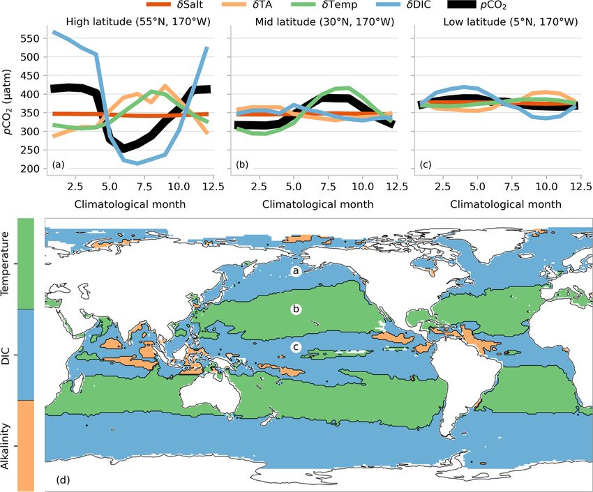
L. Gregor and N. Gruber: Surface ocean acidification data set                                                                785

mon and Dickson, 2015). However, most of the biases in the            For DIC and pH, we use the directly measured data from
cruises were corrected based on calibration to deep samples,       GLODAP v2.2019 (Olsen et al., 2019). Bockmon and Dick-
where it is assumed that interannual TA variability is negligi-    son (2015) report a measurement error of ± 5 µmol kg−1 for
ble relative to the magnitude of the bias (Olsen et al., 2019).    GLODAP DIC in an inter-laboratory comparison. Olsen et al.
These bias corrections amount to ± 5 µmol kg−1 on average.         (2019) estimate the measurement error for pH to be 0.01. To
   For the regression of pCO2 , we use SOCAT v2019 where           be consistent with TA, we select data shallower than 20 m in
only data with a SOCAT cruise quality flag of A to D and a         latitudes lower than 30◦ and shallower than 30 m at higher
World Ocean Circulation Experiment (WOCE) quality flag             latitudes and resampled the data to monthly by 1◦ × 1◦ .
of 2 are used. As is the case for TA, we do not exclude               Three long-term time series stations are used to provide
data from coastal and nearshore environments. The fugac-           direct independent comparisons for DIC and TA, namely
ity of CO2 (f CO2 ) reported in SOCAT v2019 is converted           the Hawaii Ocean Time-series at 22.57◦ N, 158◦ W (HOT,
to pCO2 using                                                      Dore et al., 2009); the Bermuda Atlantic Time-series Study
                                                                 at 32◦ N, 64◦ W (BATS, Bates and Peters, 2007); and the
                                 B +2·δ
pCO2 = f CO2 · exp Patm  surf
                              ·               ,             (1)    Irminger station in the high northern Atlantic (64.3◦ N,
                                R · T SOCAT                        28◦ W, Olafsson et al., 2010, only for DIC). The accuracy
where P is atmospheric pressure at sea level from the ERA5         for these measurements is reported to be below 2 µmol kg−1
reanalysis product (Hersbach, 2018). B and δ are virial co-        for DIC and ∼ 4 µmol kg−1 for TA for all stations. We use
efficients, R is the gas constant, and T SOCAT is the ship         the same depth constraints for the long-term stations as for
intake temperature in ◦ C (Dickson et al., 2007). In ex-           GLODAP, explained in the paragraph above. pCO2 is also
ploratory work for this study, we tested predicting 1pCO2 =        calculated from DIC and TA for HOT and BATS to provide
pCOatm                                                             an additional constraint.
      2 − pCO2 instead of just pCO2 but found that this did
not produce credible results; for a more in-depth discussion          Data present in the Lamont-Doherty Earth Observatory
see Sect. A2.                                                      pCO2 data set but not in SOCAT are used to independently
   The discrete measurements of pCO2 and TA are resam-             compare pCO2 (Takahashi et al., 2020). Takahashi et al.
pled on a monthly grid (January 1985 through Decem-                (2020) report an error estimate of ±2.5 µatm, but it must be
ber 2018) with a spatial resolution of 1◦ × 1◦ to match the        added that some of the data unique to LDEO may be ex-
predictors used in the mapping step.                               cluded from SOCAT due to stricter quality control criteria
   Finally, outliers are removed from gridded pCOSOCAT       us-   for the latter; thus errors for the LDEO data are expected to
                                                      2
ing the methods described in Sect. A1. In total, 2425 points       be larger (Bakker et al., 2016).
are removed from the gridded pCOSOCAT          using these out-       Finally, we include Argo float measurements of pH
                                       2
lier removal approaches, equivalent to 0.85 % of the original      from the Southern Ocean Carbon and Climate Observations
gridded data.                                                      and Modeling project (SOCCOM) (Johnson et al., 2017;
   We use sea-surface temperature from OSTIA for both TA           Williams et al., 2017). Johnson et al. (2016) report a mean
and pCO2 regression (Good et al., 2020). The TA model is           uncertainty of ± 0.019 for pH for the entire water column,
trained using in situ salinity from GLODAP v2, but salin-          though this is likely higher for the upper 30 m as the authors
ity from SODA v4.3.2 is used for the mapping step (Olsen           report lower errors for estimates below 50 m.
et al., 2019; Carton et al., 2018). The N ∗ and H4 SiO4 are the
same as used in the clustering step but are repeated for the
number of years. Similarly, the mixed-layer depth climatol-        2.4   Computation of DIC, pH, and Ω
ogy described in Sect. 2.3.1 is repeated for each year. We use
the global mean of the mole fraction of CO2 for the marine         The remaining parameters of the marine carbonate system,
boundary layer (xCOmbl                                             i.e., DIC, pH, and , are computed using the Python ver-
                        2 ) as a predictor in the regression, as
the correction for water vapor pressure may otherwise intro-       sion of CO2SYS (Humphreys et al., 2020) originally de-
duce co-variance with other predictors (i.e., SST, SSS). Miss-     veloped by Lewis et al. (1998). In addition to pCO2 and
ing data in the monthly GlobColour chlorophyll a product           TA, CO2SYS requires the input of sea-surface temperature,
are filled with climatological data described in Sect. 2.3.1.      sea-surface salinity, pressure (assumed 0 dbar at the surface),
The meridional and zonal components of the surface winds           PO3−4 , and H4 SiO4 . We use the same data sources described
are averaged from the hourly output from the ERA5 reanaly-         in Sect. 2.3.2 and Table 1. Climatologies of H4 SiO4 and
sis (Hersbach, 2018).                                              PO3−4 are repeated for each year, thus assuming no interan-
                                                                   nual variability. The impact of this assumption is minimal
                                                                   ( 2 µmol kg−1 ), as can be shown by varying these nutrients
2.3.3   Evaluation variables
                                                                   over seasonal cycle. The dissociation constants by Dickson
The machine learning estimates of TA, pCO2 , and the com-          et al. (1990) for KHSO4 and the total boron–salinity relation-
puted DIC and pH are evaluated against data that are not used      ship by Uppström (1974) were used, as recommended by Orr
in the training or mapping step.                                   et al. (2015) and Raimondi et al. (2019). For further details

https://doi.org/10.5194/essd-13-777-2021                                             Earth Syst. Sci. Data, 13, 777–808, 2021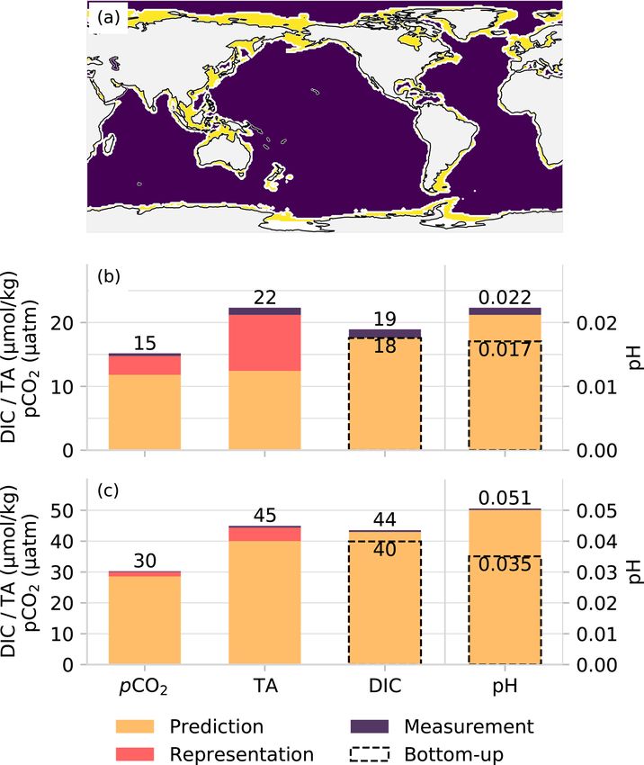
786                                                                L. Gregor and N. Gruber: Surface ocean acidification data set

on the calculation and the full description of the marine car-           The measurement error reflects the combination of poten-
bonate system, see Dickson et al. (2007).                             tial biases (systematic errors) from sampling and measure-
   An important consideration in these calculations is the in-        ment as well as random errors associated with sampling and
ternal consistency of the marine carbonate system, i.e., the          the imprecise nature of the measurement system. Since both
error due to uncertainties in the equations and coefficients          TA and pCO2 are being measured against certified reference
that describe the marine carbonate system. Raimondi et al.            materials and have undergone extensive secondary quality
(2019) pointed out that the pCO2 –TA pair has the lowest er-          control, we assume that they have no systematic error, i.e.,
ror in the calculation of pH (0.003 ± 0.008 pH units) using           that their bias is zero. We also assume the sampling error to
the dissociation constants by Mehrbach et al. (1973) as refit-        be small, so that the uncertainty M associated with the mea-
ted by Dickson and Millero (1987). However, using the same            surement error can be well approximated by the precision
pair and the same dissociation constants resulted in an es-           of the employed measurement methodology (Dickson et al.,
timate of  with respect to aragonite that is very different          2007).
from that computed using the DIC–TA pair. But since Rai-                 The representation error, R, is a result of the fact that we
mondi et al. (2019) lacked direct measurements of , it re-           develop our statistical model (GRaCER) on a grid that is in
mains unclear which pair is actually better for . We cannot          many places coarser in time and space than the typical scales
resolve this here but need to acknowledge that this inconsis-         of variability of TA and pCO2 . As a result, any given obser-
tency adds some additional uncertainty to our computed               vation may not be representative for the 1◦ ×1◦ monthly grid
values.                                                               cell used as a basis for our regression, leading to a bias in
                                                                      the estimated mean relative to the true spatial and temporal
3     Uncertainty assessment                                          mean. This problem is particularly severe if the number of
                                                                      samples within any grid cell is low and the spatiotemporal
Any application of our data product requires a firm under-            variability is high. This is often the case. For example, more
standing of the errors and uncertainties associated with each         than 90 % of the data in the monthly gridded pCO2 prod-
of the reported parameters of the surface ocean carbonate             uct are based on a single day of sampling within the month.
system. We first discuss the errors and uncertainties associ-         The situation is more dire for TA, for which there are 10-
ated with the statistically modeled quantities TA and pCO2            fold fewer observations than pCO2 . Since we are lacking full
and then those with the computed parameters DIC, pH, and              knowledge of the spatial and temporal variability of TA and
. Then, we will compare these propagated uncertainties               pCO2 , we cannot fully quantify the representation error. In-
with the uncertainty of the computed DIC and pH by com-               stead, we approximate it using the few regions where we have
paring these values with in situ observations. This provides          sufficient observations or then using closely related parame-
a strong check on our ability to establish a full uncertainty         ters for which we have more observations. For simplicity, we
budget. Here, we use the term “uncertainty” to characterize           make the assumption that the uncertainty associated with this
the range of values within which the true value is asserted to        error is, on a global average, normally distributed with a bias
lie with some level of confidence. The term “error” is used           of 0.
in two ways: first, as a process that leads to deviations be-            The uncertainty associated with the prediction error, P ,
tween the measurement and the true value and, second, as              is determined by the test scores from the evaluation of the
an estimate quantifiable against a known value. For the pur-          statistical model vis-à-vis the independent test data. The test
pose of our analysis here, we consider the training data sets         scores describe the error incurred in the prediction of the sub-
for TA and pCO2 as such known values; i.e., we assume that            set of data that are not used in the training step. This error
these observations are unbiased. This can be justified on the         includes also the propagated uncertainty associated with the
basis of their having undergone extensive secondary quality           predictor variables.
control.                                                                 We Psummarize these uncertainties with mean bi-
                                                                                  N
                                                                                      (ŷ −y )
                                                                      ases ( i=1N i i ) and root mean squared error (RMSE,
                                                                      q PN
                                                                                         2
3.1    Sources of errors for TA and pCO2                                   i=1 (ŷi −yi )
                                                                                           ), where y is the target value, ŷ is the predicted
                                                                                N
We identify three sources of errors that contribute to the total      value, and N is the number of observations. We separate the
uncertainty for pCO2 and TA, namely the uncertainty stem-             coastal and open-ocean regions using the COastal Segmen-
ming from the measurement (M), representation (R), and                tation and related CATchments (COSCATs) mask (Laruelle
prediction (P ) errors. Assuming independence of the three            et al., 2013) in order to reflect their very different levels of
error sources, the total uncertainty (E) for the TA and pCO2          spatiotemporal variability.
estimates can thus be expressed as the root of the squared
sum of the uncertainties from the three error sources:                3.1.1    Uncertainty for total alkalinity
     p
E = M 2 + R2 + P 2.                                          (2)      We adopt an uncertainty M associated with the measurement
                                                                      error of TA of ± 5 µmol kg−1 based on the laboratory inter-

Earth Syst. Sci. Data, 13, 777–808, 2021                                                  https://doi.org/10.5194/essd-13-777-2021
L. Gregor and N. Gruber: Surface ocean acidification data set 787
Table 3. Summary of the uncertainties of total alkalinity and pCO2 from the different error sources (see Table 2) separately evaluated for the
open ocean and for coastal regions (defined by the COSCATs regions, Laruelle et al., 2013). See text for details on how the different sources
were quantified.
Alkalinity (µmol kg−1 ) pCO2 (µatm)
Uncertainty Open Coastal Open Coastal
ocean ocean
Measurement 5 (≤ 10) 2 (≤ 5)
Representation 16 34 7 17
Prediction 13 28 12 27
Total 21 45 14 32
comparison by Bockmon and Dickson (2015). This is only and climatologically mapped test errors for TA in Fig. A2
half the accuracy of ± 10 µmol kg−1 or 0.5 % reported by using the GRaCER approach.
GLODAPv2 (Olsen et al., 2019). We consider this to be an While the global bias of the TA product of OceanSODA-
overly conservative estimate, since Bockmon and Dickson ETHZ is near zero (0.5 µmol kg−1 ), confirming our assump-
(2015) pointed out that the majority of the laboratories in- tion about the unbiased nature of our prediction error, this
volved in the round-robin exercise achieved an accuracy of is not the case regionally. For example, OceanSODA-ETHZ
better than ± 5 µmol kg−1 . We thus opted for this lower value tends to consistently overestimate TA in the southeastern At-
that is more representative of the majority of the data. lantic and underestimate TA in the southern Indian Ocean
Owing to the sparseness of the TA observations, we cannot (Fig. 3b). A seasonal breakdown of the biases into DJF and
estimate the uncertainty R associated with the representation JJA reveals that the winter period of each hemisphere has bi-
error directly. Instead, we use the high correlation between ases in the high latitudes, though the paucity of data means
TA and salinity. This permits us to determine the representa- that we can place less weight on this finding.
tion error for TA indirectly from an estimate of the represen- A good check on the model prediction error is provided
tation error of sea-surface salinity. Concretely, we compare by comparing the estimated TA against independent obser-
the test RMSE of TA predicted with GLODAPv2’s in situ vations. To this end, we use data from the Hawaii Ocean
salinity with the RMSE of TA predicted with the satellite- Time-series (HOT), the Bermuda Atlantic Time-series Study
based SODA salinity (see Table 1). Since the latter salinity (BATS), and the Irminger station shown in Fig. 4a, b, e, f,
is supposed to reflect the true time–space average over each i, and j and Table 4. For the period 1990–2018, the bias for
grid cell, the difference between these two salinities is a di- BATS is 3 µmol kg−1 and for HOT −2 µmol kg−1 , indicat-
rect estimate of the uncertainty associated with the represen- ing that the method captures the overall structure and vari-
tation error for salinity. Consequently, the difference in TA ability of TA well at these subtropical stations. Further, the
from these two estimates is an estimate of the uncertainty as- mean seasonal cycle is relatively well represented at HOT
sociated with the representation error for TA. The resulting and BATS, being within 1 standard deviation of the interan-
estimates for the open and coastal ocean are summarized in nual variability when averaged as a climatology (Fig. 4b, f).
Table 3. However, the results are not as good for the Irminger station
The uncertainty P associated with the prediction error is in the Atlantic high latitudes (∼ 65◦ N), where OceanSODA-
based on the model’s RMSE score calculated from test data ETHZ has a large negative bias (−10 µmol kg−1 ) when com-
and is listed in Table 3 and Fig. 3a. The global mean predic- pared to TA computed from the observed pCO2 and DIC.
tion error for the open ocean amounts to 13 µmol kg−1 , with OceanSODA-ETHZ also overestimates the weak seasonal
some regional differences. The prediction error is more than cycle of TA at the Irminger station, contributing to the
twice this number in the coastal regions, i.e., 28 µmol kg−1 large bias that is particularly strong from December to May.
(coastal regions are defined by the COSCATs regions, Laru- The RMSE at Irminger station is 15 µmol kg−1 , less than
elle et al., 2013). We find especially high prediction errors, 5 µmol kg−1 larger than the RMSE for HOT and BATS sta-
for example, in the highly dynamic Amazon outflow region tions (10 µmol kg−1 respectively) owing to the small inter-
or the Gulf of Maine in the northwestern Atlantic. However, annual and seasonal amplitude at Irminger. The RMSEs are
in such regions, one can expect that part of the high predic- thus smaller than the mean prediction error (13 µmol kg−1 ) at
tion error is actually stemming from a representation error, the subtropical stations yet exceed this mean estimate at the
as we are not using directly co-measured variables when we high-latitude station.
train our regression model. In Fig. A2, we show the spatially
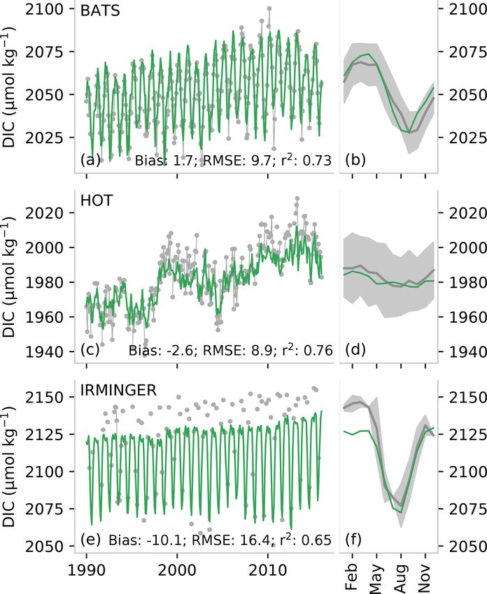
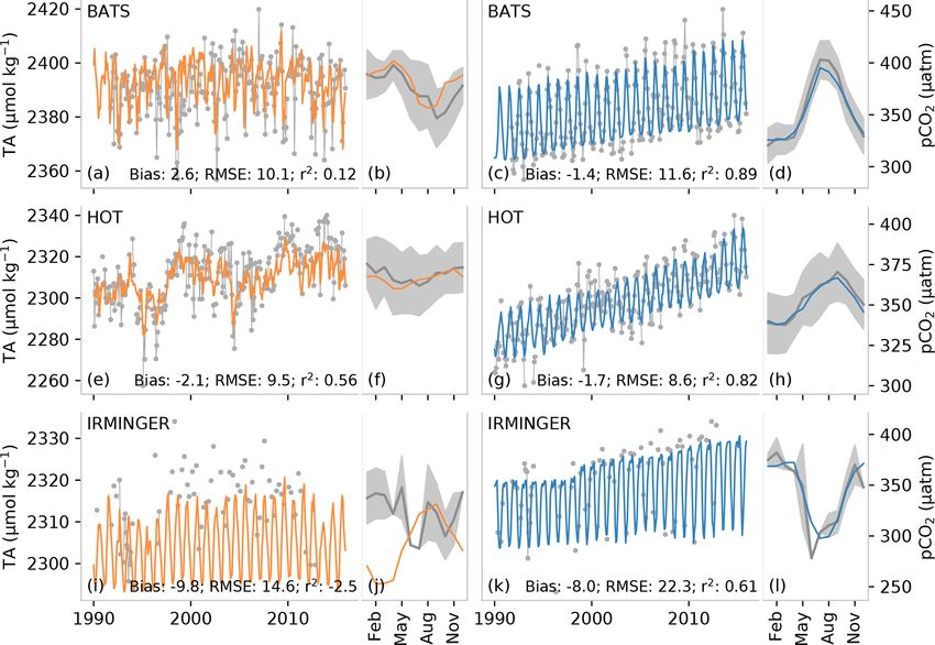
https://doi.org/10.5194/essd-13-777-2021 Earth Syst. Sci. Data, 13, 777–808, 2021788 L. Gregor and N. Gruber: Surface ocean acidification data set Figure 3. Test metrics for total alkalinity (a, b) and pCO2 (c, d). The left-hand column (a, d) shows the root mean squared error (RMSE) compared with the target data. Similarly, the middle column (b, e) shows bias compared to the respective training data sets (GLODAP v2.2019 and SOCAT v2019). The right-hand column shows the zonally averaged biases for June, July, and August (JJA, blue) and December, January, and February (DJF, orange). A 2D spatial convolution was first applied to the 1◦ ×1◦ pixels to make regional patterns in the biases and RMSE clearer, and data were then aggregated into 4◦ × 4◦ pixels for clearer visualization. Figure 4. A comparison of a subset of measurements from long-term observation stations (gray) with predicted total alkalinity (TA) (a, b, e, f, i, j) and partial pressure of CO2 (pCO2 ) (c, d, g ,h, k, l). The top row (a–d) shows data for the Bermuda Ocean Time-series Study (BATS), the middle row (e–h) shows data for the Hawaii Ocean Time-series (HOT), and the bottom row (i, l) shows data for the Irminger station. The narrow panels show the average of the seasonal climatology for the time series. The gray shading shows the standard deviation of the observations for the period 1990 to 2018, while the orange/blue lines show the average estimate. TA for the Irminger station is calculated from pCO2 and DIC, and pCO2 is calculated for BATS and HOT using DIC and TA, as described in Sect. 2.4. Earth Syst. Sci. Data, 13, 777–808, 2021 https://doi.org/10.5194/essd-13-777-2021
L. Gregor and N. Gruber: Surface ocean acidification data set                                                                              789

Table 4. Comparison of training and independent data sources with various methods for the open-ocean region using the COSCATs coastal
mask by Laruelle et al. (2013). GLODAP refers to the GLODAP v2 2019 data (Olsen et al., 2019), HOT refers to the Hawaii Ocean Time-
series (Dore et al., 2009), BATS refers to Bermuda Atlantic Time-series Study (Bates and Peters, 2007), SOCAT is the 2019 version of the
Surface Ocean Carbon Atlas (Bakker et al., 2016), LDEO is the Lamont-Doherty Earth Observatory pCO2 data set for points not present
in SOCAT (Takahashi et al., 2020), and SOCCOM is the pH measured by autonomous floats from the Southern Ocean Carbon and Climate
Observations and Modeling project (Johnson et al., 2016). Statistical outliers were excluded in the calculation of LDEO RMSE. OS-ETHZ
is the OceanSODA-ETHZ data from this study, NNGv2 is from Broullón et al. (2018), LIARv2 from Carter et al. (2018), CMEMS-FFNNv2
from Denvil-Sommer et al. (2019), and SOMFFN from Landschützer et al. (2016). NNGv2 and LIARv2 predictions are made with SODA
salinity and OSTIA sea-surface temperature, resulting in different estimates to the original publications (Broullón et al., 2018; Carter et al.,
2018). Note that the full data set is used for OceanSODA-ETHZ, unlike Table 3, which presents the errors for test years.

                                     TA (µmol kg−1 )             pCO2 (µatm)              DIC (µmol kg−1 )                        pH
                               GLODAP       HOT      BATS      SOCAT      LDEO       GLODAP        HOT     BATS      GLODAP        SOCCOM
 Bias       this study                0.5   −2.1        2.6       −0.4        0.1           0.5    −1.0       0.4       −0.001          0.009
            LIAR + FFNN               0.3   −3.1        0.2        0.5        0.6                                        0.001          0.013
            NNGv2                     1.2   −3.2        4.3                                 2.3      2.2     −0.4
            SOMFFN                                                  0.4       0.4
 RMSE       this study               17.5     9.5      10.1       11.1       19.9          16.3      8.7      9.1         0.024         0.036
            LIAR + FFNN              18.0     8.8       8.8       13.1       19.6                                         0.023         0.037
            NNGv2                    16.2     6.7      10.4                                23.1      9.5     15.2
            SOMFFN                                                11.7       21.4
 r2         this study               0.91    0.58      0.13       0.82       0.45          0.93    0.77      0.76          0.67         0.047
            LIAR + FFNN              0.91     0.6      0.21       0.78       0.44                                          0.67        −0.043
            NNGv2                    0.93    0.75      −0.1                                0.82    0.71      0.38
            SOMFFN                                                0.82       0.49

3.1.2   Uncertainty for pCO2                                              with the highest variance in the observations. The strong hor-
                                                                          izontal gradients in the region increase the errors, particu-
                                                                          larly at cluster boundaries. The high RMSE for the coastal
For the uncertainty M associated with the measurement error
                                                                          region stems primarily from coastal Antarctica as well as
of pCO2 , we adopt a value of ±2 µatm. This reflects the fact
                                                                          some coastal regions in the higher latitudes of the North-
that 80 % of the data we have used from SOCAT (flags A and
                                                                          ern Hemisphere. The former is due to large uncertainties in
B) have a precision better than that number and an accuracy
                                                                          pCO2 during the summer months when retreating ice and en-
of similar magnitude. The remaining data we used (SOCAT
                                                                          suing rapid net primary production result in large gradients
flags C and D) have a measurement precision and accuracy
                                                                          (Bakker et al., 2008). The climatologically mapped errors for
of less than ±5 µatm.
                                                                          pCO2 are shown in Fig. A2b and d, created by mapping the
   We estimate the uncertainty R associated with the repre-
                                                                          test errors to the clusters and averaged over the ensemble.
sentation error of pCO2 on the basis of a spatiotemporal gra-
                                                                             The comparison between the regression estimated and ob-
dient analysis. To this end, we compare the pCO2 in our reg-
                                                                          served pCO2 reveals regional biases (Fig. 3e), despite the
ular grid that has a resolution of 1◦ × 1◦ by 1 month, with
                                                                          global bias being close to zero (−0.37 µatm). Some of the
the pCO2 binned to a grid with twice this resolution, i.e.,
                                                                          highest biases are found, again, in the eastern tropical Pa-
0.5◦ × 0.5◦ by 15 d. In regions with high spatiotemporal cov-
                                                                          cific, where strong horizontal gradients drive the observed
erage, the difference in the average of adjacent grid cells rep-
                                                                          juxtaposed biases. The large negative biases in winter in the
resents the potential change that can occur within the coarser
                                                                          Southern Ocean are likely driven by the paucity of data in
1◦ × 1◦ by a 1-month grid cell. The spatial and temporal gra-
                                                                          this region (Gregor et al., 2019; Gray et al., 2018; Bushinsky
dients are calculated separately, and we take the average of
                                                                          et al., 2019).
these two elements. Using this analysis, we estimate a repre-
                                                                             The time series comparisons show that the seasonal cy-
sentation error of our pCO2 estimates of 7 and 17 µatm for
                                                                          cle is well represented at BATS and HOT with r 2 scores of
the open and coastal ocean respectively (Table 3).
                                                                          0.89 and 0.82 respectively (Fig. 4d, h). Low biases (< 2 µatm
   From the RMSE of our test data, we estimate an uncer-
                                                                          in absolute terms) further demonstrate that pCO2 estimates
tainty P associated with the prediction error of pCO2 of
                                                                          are reliable in the subtropics. The seasonal cycle is also well
12 µatm for the open ocean and 28 µatm for the coastal ocean
                                                                          captured at the Irminger station in the high latitudes, but a
(Table 3). Within the open ocean (Fig. 3e), the eastern tropi-
                                                                          lower r 2 score and larger bias (−8.0 µmol kg−1 ) allude to the
cal Pacific has the highest RMSE, but this is also the region

https://doi.org/10.5194/essd-13-777-2021                                                      Earth Syst. Sci. Data, 13, 777–808, 2021
You can also read