The Data Processing Pipeline for the MUSE Instrument
←
→
Page content transcription
If your browser does not render page correctly, please read the page content below
Astronomy & Astrophysics manuscript no. pipeline                                                                                     c ESO 2020
                                               June 17, 2020

                                                             The Data Processing Pipeline for the MUSE Instrument
                                               Peter M. Weilbacher1 , Ralf Palsa2 , Ole Streicher1 , Roland Bacon3 , Tanya Urrutia1 , Lutz Wisotzki1 , Simon Conseil3, 4 ,
                                                 Bernd Husemann5 , Aurélien Jarno3 , Andreas Kelz1 , Arlette Pécontal-Rousset3 , Johan Richard3 , Martin M. Roth1 ,
                                                                                         Fernando Selman6 , and Joël Vernet2

                                                     1
                                                         Leibniz-Institut für Astrophysik Potsdam (AIP), An der Sternwarte 16, 14482 Potsdam, Germany
                                                         e-mail: pweilbacher@aip.de
                                                     2
                                                         ESO, European Southern Observatory, Karl-Schwarzschild-Str. 2, 85748 Garching bei München, Germany
                                                     3
                                                         Univ Lyon, Univ Lyon1, Ens de Lyon, CNRS, Centre de Recherche Astrophysique de Lyon UMR5574, F-69230, Saint-Genis-
                                                         Laval, France
                                                     4
                                                         Gemini Observatory / NSF’s OIR Lab, Casilla 603, La Serena, Chile
arXiv:2006.08638v1 [astro-ph.IM] 15 Jun 2020

                                                     5
                                                         Max-Planck-Institut für Astronomie, Königstuhl 17, 69117 Heidelberg, Germany
                                                     6
                                                         European Southern Observatory, Ave. Alonso de Córdova 3107, Vitacura, Santiago, Chile

                                                    Received 29 February 2020 / accepted 13 June 2020

                                                                                                                 ABSTRACT

                                                    Processing of raw data from modern astronomical instruments is nowadays often carried out using dedicated software, so-called
                                                    “pipelines” which are largely run in automated operation. In this paper we describe the data reduction pipeline of the Multi Unit
                                                    Spectroscopic Explorer (MUSE) integral field spectrograph operated at ESO’s Paranal observatory. This spectrograph is a complex
                                                    machine: it records data of 1152 separate spatial elements on detectors in its 24 integral field units. Efficiently handling such data
                                                    requires sophisticated software, a high degree of automation and parallelization. We describe the algorithms of all processing steps
                                                    that operate on calibrations and science data in detail, and explain how the raw science data gets transformed into calibrated datacubes.
                                                    We finally check the quality of selected procedures and output data products, and demonstrate that the pipeline provides datacubes
                                                    ready for scientific analysis.
                                                    Key words. instrumentation: spectrographs – techniques: imaging spectroscopy – methods: observational – methods: data analysis

                                               1. Introduction                                                            performance requirements, six were relevant for the develop-
                                                                                                                          ment of the pipeline. They included (i) the capability to recon-
                                               MUSE (the Multi-Unit Spectroscopic Explorer; Bacon et al.                  struct images with a precision of better than 1/4 pixel, (ii) a flux
                                               2010; Bacon et al. 2014) is a large-field, medium resolution inte-         calibration accurate to ±20%, (iii) the ability to support offsets,
                                               gral field spectrograph operated at the European Southern Obser-           (iv) sky subtraction to better than 5% sky intensity outside the
                                               vatory (ESO) Very Large Telescope (VLT) since October 2014.                emission lines, with a goal of 2%, (v) the capability to combine
                                                                                                                          up to 20 dithered exposures with a S/N of at least 90% of the
                                               1.1. Historical background                                                 theoretical value, and (vi) a wavelength calibration accuracy of
                                                                                                                          better than 1/20th of a resolution element. Overall, the goal was
                                               MUSE was developed as one of the 2nd generation instruments                to deliver software that would generate data cubes ready for sci-
                                               at ESO’s Paranal observatory. At its inception, the landscape              entific use, with the best possible S/N to detect faint sources,
                                               of optical integral field spectrographs was led by a few in-               with only minimal user interaction. More details of the history
                                               struments at 4 m-class telescopes, like SAURON (Bacon et al.               of 3D spectroscopic instruments, their properties, and the devel-
                                               2001) and PMAS (Roth et al. 2005), as well as fiber-based                  opment of MUSE can be found in Bacon & Monnet (2017).
                                               units like VIMOS (Le Fèvre et al. 2003) and GMOS (Allington-
                                               Smith et al. 2002) on 8 m telescopes. While the Euro3D net-
                                               work (Walsh 2004) had been created to develop software for
                                                                                                                          1.2. Instrument properties
                                               such instruments (Roth 2006), data reduction remained cumber-
                                               some (e. g., Monreal-Ibero et al. 2005). Depending on obser-
                                               vatory and instrument in question, only basic procedures were              In its wide-field mode (WFM), the instrument samples the sky
                                               widely available. While there were exceptions (Wisotzki et al.             at approximately 000. 2 × 000. 2 spatial elements and in wavelength
                                               2003; Zanichelli et al. 2005, among others), researchers often             bins of about 1.25 Å pixel−1 at a spectral resolution of R ∼ 3000
                                               struggled to subtract the sky and to combine multiple expo-                over a 10 × 10 field of view with a wavelength coverage of at least
                                               sures, and many homegrown procedures were developed to do                  4800. . . 9300 Å (nominal) and 4650. . . 9300 Å (extended mode).
                                               that and produce datacubes ready for analysis. The results were            Since 2017, MUSE can operate with adaptive optics (AO) sup-
                                               frequently suboptimal (e. g., van Breukelen et al. 2005).                  port (Ströbele et al. 2012). In WFM, it is operated in a seeing-
                                                   In this environment, the specifications for MUSE were de-              enhancing mode, correcting the ground layer only (see Kamann
                                               veloped by ESO based mostly on the experience with the                     et al. 2018a, for a first science result), the pixel scale and wave-
                                               FLAMES/GIRAFFE spectrograph (Pasquini et al. 2002). Of the                 length range stay the same.
                                                                                                                                                                     Article number, page 1 of 31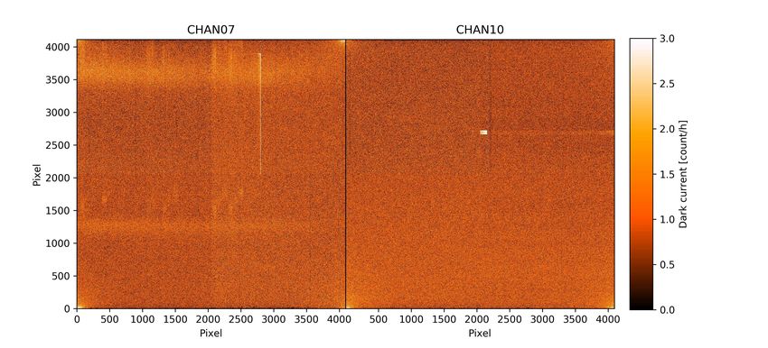
A&A proofs: manuscript no. pipeline

      A high-order laser tomography AO correction (Oberti et al.                          science exposure
                                                                                                                   pixel table

2018) has been available in the so-called Narrow Field Mode
(NFM) since 2018 (Knapen et al. 2019; Irwin et al. 2019, are                                                        merge IFUs
first science publications). In this mode, the scale is changed to      bad pixel table
                                                                                              mark bad
25 mas pixel−1 to better sample the AO-corrected point spread                                  pixels
                                                                                                                      correct
function (PSF). The resulting field is then 8× smaller (about                                                        refraction
700. 5 × 700. 5). The wavelength range is the same as in nominal                                                                           response
                                                                                                bias
mode. In all these cases, the data is recorded on a fixed-format       master bias
                                                                                             subtraction           flux calibrate          telluric
array of 24 CCDs (Charge Coupled Devices), each of which is                                                                         extinction curve
read out to deliver raw images of 4224 × 4240 pixels in size. We                                                     subtract
                                                                       master dark            subtract                                   raman lines
summarize the instrument modes in Table A.1 and show a sketch                                   dark                  Raman

of its operation in Fig. B.1.
      For an instrument with such complexity, combined with the                                                    self-calibrate               mask
                                                                                              divide by
size of the raw data (about 800 MB uncompressed), a dedicated          master flat
                                                                                              flat-field
                                                                                                                                         sky lines
processing environment is a necessity. This pipeline was there-                                                      subtract
                                                                       tracing                                                         sky continuum
fore planned early-on during the instrument development to be                                                          sky

an essential part of MUSE. While some design choices of the in-        wavelengths
                                                                                               create                                 line profile
                                                                                             pixel table
strument were mainly driven by high-redshift Universe science                                                         correct
                                                                       geometry                                      velocities
cases, many other observations were already envisioned before
the start of MUSE observations. By now MUSE actually evolved           illumination         illumination              correct
                                                                           flat                                                         astrometry
into a general purpose instrument, as documented by recent pub-                               correction            distortions

lications on the topics of (exo-)planets (Irwin et al. 2018; Haffert
et al. 2019), Galactic targets (Weilbacher et al. 2015; McLeod                                                      set position            offsets

et al. 2015), and resolved stellar populations (Husser et al. 2016;        skyflat          apply skyflat

Kamann et al. 2018b), via nearby galaxies (Krajnović et al. 2015;                                                   combine
Monreal-Ibero et al. 2015) and galaxy clusters (Richard et al.                                                      exposures

2015; Patrício et al. 2018) to high-redshift Lyman-α emitters                                create flat
                                                                                             spectrum
(Bacon et al. 2015; Wisotzki et al. 2016, 2018), to name only                                                        resample

a few science applications. In contrast to some other instruments
with a dominating scientific application (see Strassmeier et al.
                                                                                            pixel table             data cube
2015; Scott et al. 2018), the MUSE pipeline thus cannot be con-
cerned with astrophysical analysis tasks. Its role is confined to
the transformation from the raw CCD-based data to fully cali-          Fig. 1. Left: Basic processing from raw science data to the intermedi-
brated data cubes. Depending on the science case in question,          ate pixel table. Right: Post-processing from pixel table to the final dat-
other tools were then created to handle the data cubes (MUSE           acube. Optional steps are marked grey, mandatory ones in blue. Man-
Python Data Analysis Framework, MPDAF, Bacon et al. 2016;              ually created input files have an orange background, calibrations are
                                                                       highlighted. Inputs that are needed are connected with a solid line, dot-
Piqueras et al. 2019), to extract stellar (PampelMUSE, Kamann          ted lines signify inputs that are not required.
et al. 2013) or galaxy (TDOSE, Schmidt et al. 2019) spectra, or
to detect emission lines sources (LSDCat, Herenz & Wisotzki
2017), among others. Describing these external tools is not the
                                                                       all modes of the instrument, in particular the NFM.2 Where ap-
purpose of this paper.
                                                                       plicable, we note in which version a new feature was introduced.

1.3. Paper structure
The data processing of MUSE at different stages of implementa-         2. Science processing overview
tion was previously described in Weilbacher et al. (2009), Stre-
icher et al. (2011), Weilbacher et al. (2012), and Weilbacher et al.   The main processing steps to calibrate the data and transform it
(2014). These papers still reflect much of the final pipeline soft-    from the image-based format of the raw data via a table-based
ware, and explain some of the design choices in more detail. The       intermediate format during processing to the output cube are vi-
present paper aims to first describe the science processing steps      sualized in Fig. 1. The computations are split into two parts, the
on a high level (Sect. 2) to let the user get an idea of the steps     basic processing – this calibrates and corrects data on the basis
involved in the aforementioned transformation. Afterwards, in          of single CCDs – and the post-processing – carrying out on-sky
Sect. 3, we give a detailed description of all steps involved in       calibrations and construction of the final datacube. The interme-
generating master calibrations and science products. Some al-          diate data, the pixel tables, are the files that connect both pro-
gorithms that are used in multiple steps are then presented in         cessing levels.
Sect. 4 while Sect. 5 briefly discusses key parameters of the               In this section, we only briefly mention the processing steps,
implementation. Sect. 6 investigates the data quality delivered        and point to later sections where they are described in more de-
by the pipeline processing. We conclude with a brief outlook in        tail. In a few cases a processing step is not connected to a cal-
Sect. 7.                                                               ibration file, and hence not described further. Then we describe
    This paper is based on MUSE pipeline version 2.8.3 as pub-         this step here in greater depth.
licly released in June 20201 . v2.8 was the first version to support
                                                                       2
                                                                           Milestones of earlier versions were v1.0 in Dec. 2014 to support the
1
  https://www.eso.org/sci/software/pipelines/muse/                     first observing runs with only seeing-limited WFM, and v2.2 which first
muse-pipe-recipes.html                                                 supported WFM AO data in Oct. 2017.

Article number, page 2 of 31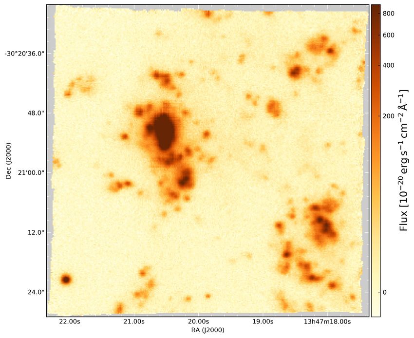
Weilbacher et al.: The Data Processing Pipeline for the MUSE Instrument
is read in (DATA image) from the raw data (the corresponding
CHANnn extension), and two images of the same size are added,
one for the data quality (DQ, see Sect. 4.2), one for the variance
(STAT, see Sect. 4.1). Both new images are empty at the start.
Next, if the optional bad pixel table was given, those pixels are
marked in the DQ image. In any case, saturated pixels are detected
and marked, if the data allow such determination to be made (raw
values zero or above 65500).
Next, the overscan regions of the MUSE CCDs are analyzed
to determine corrective factor and slopes to apply to the bias
(see Sect. 4.3 for more details about this step), before the mas-
ter bias image of the corresponding CCD is subtracted. Then,
the CCD gain is used to transform the input data from analog-
to-digital units (adu) to electrons (internally called count). The
gain value is taken from the FITS headers of the raw exposure.
If the optional master dark was given, the pipeline subtracts the
dark current image given by that calibration file. An optional step
in the CCD-level calibration is to detect and mark cosmic rays
(using the DCR algorithm, Pych 2004). However, this is usually
not necessary at this stage (as explained in detail in Sect. 4.5.1).
The science image is then divided by the master lamp flat-field
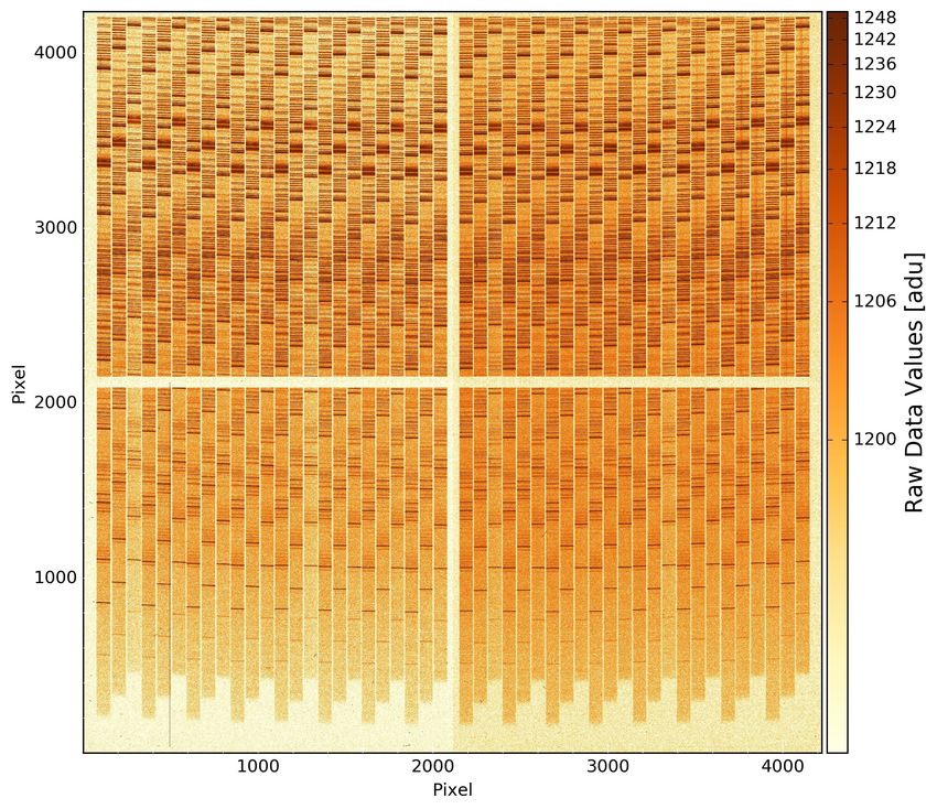
Fig. 2. Raw science data of one of the 24 CCDs, displayed in negative
arcsinh scaling. This shows the data of IFU 10 of the exposure started image provided to the processing routine. The last step in the di-
at 2014-06-26T01:24:23 (during MUSE Science Verification). The 48 rect CCD-level processing propagates the relative IFU flux level
slices of the IFU are the stripes oriented almost vertically, that appear from the twilight sky cube, if this optional calibration was given
dark in this representation. The blue end of the MUSE wavelength range as input calibration file.
is located at the bottom, the red limit near the top, the step-pattern is The mandatory input calibrations, trace table, wavelength
created by the geometry of the image slicer. Since this was a 600 s ex- calibration table, and geometry table (their content and purpose
posure, the sky emission and continuum dominate over the relatively are explained in Sects. 3.4, 3.5, and 3.6), are used to assign co-
faint object signal in this part of the cube. The overscan regions of the ordinates – two spatial components in pseudo pixel units relative
CCDs are creating the cross in the center of the image, the prescan re- to the MUSE field of view, and one wavelength component – to
gions are the empty borders. This exposure was taken in nominal mode
(WFM-NOAO-N), the 2nd-order blocking filter removed the blue light,
each CCD-based pixel. Thereby, a pixel table is created for each
so that the bottom part of the image appears empty. input science (on-sky) exposure.
All these steps are also applied in the same way to the op-
tional raw illumination flat-field exposure if one was supplied.3
2.1. Raw data The following steps are exclusively applied to exposures taken
on-sky at night.
The MUSE raw data comes in multi-extension FITS (Flexible The wavelength zeropoint is corrected using sky emission
Image Transport System) files, where each of the 24 CCD im- lines, if applicable (see Sect. 3.5.2). Afterwards, the pixel table
ages is stored in one extension. Each of the images is 4224 × is usually cropped to the useful wavelength range, depending
4240 pixels in size, and stored as unsigned integers of 16 bit. The on the mode used for the observations. The useful wavelength
CCD is read-out on four ports, so that the CCD has four regions is defined by the range for which the MUSE field of view is
of equal size, called quadrants. These quadrants have a data sec-
fully sampled. It extends from 4750. . . 9350 Å for the nominal
tion of 2048 × 2056 pixels, and pre- and overscan regions of 32
pixels in width. The images are accessible in the FITS files via and 4600. . . 9350 Å for the extended mode.4
extension names, formed by the IFU number prefixed by CHAN, If the optional raw illumination flat-field exposure was given
for example, CHAN01 for the first IFU. A typical raw science im- as input, it is then used to correct the relative illumination be-
age of CHAN10 is displayed in Fig. 2. tween all slices of one IFU. For this, the data of each slice is
Several additional FITS extensions may be present for on- multiplied by the normalized median flux (over the wavelength
sky data, depending on the instrument mode used for an expo- range 6500. . . 7500 Å, to use the highest S/N data in the middle
sure. These are concerned with ambient conditions, performance of the wavelength range) of that slice in that special flat-field ex-
of the auto-guiding system of the VLT, the slow-guiding system posure. Since the illumination of the image slicer changes with
of the MUSE instrument, and the atmospheric turbulence param- time and temperature during the night, this correction removes
eters used by the AO system. These extra extensions are not used these achromatic variations of the illumination and thereby sig-
by the MUSE pipeline. nificantly improves flux uniformity across the field.
The last step in the basic science processing interpolates the
master twilight sky cube (Sect. 3.7, if it was given as input) to the
2.2. Basic science processing coordinate of each pixel in the pixel table. Spatially, the nearest
neighbor is taken, in wavelength a linear interpolation between
The first step of the science processing is done with the mod-
ule muse_scibasic. The inputs to this recipe are one or more 3
This illumination flat-field is a lamp-flat exposure that is taken by
raw science exposures, optionally one corresponding illumina- the observatory at least once per hour, or if the ambient temperature
tion flat-field exposure, and a number of calibration files. Out- changes significantly.
puts are pre-reduced pixel tables. 4
The exact ranges are slightly different for the AO modes, see Table
Processing is internally performed on each individual CCD, A.1. For those, the region affected by the NaD narrow-band blocking
so that all of the following is done 24 times. The raw CCD image filter is also specially marked at this stage.
Article number, page 3 of 31
A&A proofs: manuscript no. pipeline

adjacent planes is carried out. The data values in the pixel table
are then divided by the interpolated twilight sky correction.
    At this stage, the pre-reduced pixel table for each on-sky ex-
posure is saved to disk, in separate files for each IFU, including
the corresponding averaged lamp flat spectrum in one of the file
extensions.
    The module discussed in this section, muse_scibasic, is
also used to process other, non-science on-sky exposures taken
for calibration purposes. Specifically, standard star fields, sky
fields, and astrometric exposures of globular clusters are handled
by muse_scibasic, but then further processed by specialized
routines.

2.3. Science post-processing
The input to the post-processing are the pre-reduced pixel tables,
the main output is the fully reduced data cube. The first step is to
merge the pixel tables from all IFUs into a common table. This
step has to take into account the relative efficiency of each IFU
as measured from twilight sky exposures. It is applied as scaling          Fig. 3. Reduced science data. A combination of three science exposures
factor relative to the first channel. When merging the (science)           taken on 2014-06-26 between 1:00 and 2:00 UTC, including the im-
data, all lamp flat spectra of the IFUs are averaged as well. Since        age displayed in Fig. 2. This image shows a cut of the data cube at the
removing the large-scale flat-field spectrum from the (science)            wavelength of Hα (redshifted to 6653.6 Å), displayed in negative arc-
                                                                           sinh scaling. Regions at the edge that were not covered by the MUSE
data is desirable, without re-introducing the small-scale varia-           data are displayed in light grey.
tions corrected for by flat-fielding, this mean lamp flat spectrum
is smoothed over scales larger than any small-scale features like
telluric absorption or interference filter fringes. The on-sky data             The science data is then corrected for the motion of the tele-
is then divided by this spectrum.5                                         scope. This radial velocity correction is done by default relative
     Then, the merged pixel table is put through several correc-           to the barycenter of the solar system, but for special purposes he-
tions. The atmospheric refraction is corrected (for WFM data,              liocentric and geocentric corrections are available. Algorithms
the NFM uses an optical corrector) relative to a reference wave-           from G. Torres (bcv) and the FLAMES pipeline (Mulas et al.
length (see Sect. 4.8). In case a response curve is available, the         2002) and transformations from Simon et al. (1994) are used to
flux calibration is carried out next. It converts the pixel table data     compute the values.
(and variance) columns into flux units. This uses an atmospheric                The spatial coordinate correction is applied in two steps and
extinction curve that has to be passed as input table. If a tel-           makes use of the astrometric calibration (Sect. 3.12). First, linear
luric correction spectrum was provided, this is applied as well            transformation and rotation are applied and the spherical projec-
(Sect. 4.9.)                                                               tion is carried out. This transforms the pixel table spatial coor-
     For exposures taken with AO in WFM, a correction of at-               dinates into native spherical coordinates, following Calabretta &
mospheric emission lines caused by Raman scattering of the                 Greisen (2002). The second step is the spherical coordinate ro-
laser light can be carried out (see Sect. 3.10.1). A per-slice             tation onto the celestial coordinates of the observed center of
self-calibration can be run next to improve background unifor-             the field. This step can be influenced to improve both absolute
mity across the field of view of MUSE (explained in detail in              and relative positioning of the exposure by supplying coordinate
Sect. 3.10.2).                                                             offsets. Such offsets can be computed manually by the user or
     Typically, sky subtraction is carried out next. This step has         automatically by correlating object detections in overlapping ex-
multiple ways of deriving the sky contribution which also de-              posures (Sect. 3.13).
pends on the user input and the type of field being processed                   Once all these corrections and calibrations are applied on the
(sky subtraction is not needed for all science cases and can be            pixel table level, the data are ready to be combined over multiple
skipped). In case of a filled science field, an offset sky field has       exposures. This can be a very simple concatenation of the indi-
to be used to characterize the sky background (see Sect. 3.9.2             vidual pixel tables or involve relative weighting. By default, only
and 3.9.3), sky lines and continuum are then needed as inputs.             linear exposure time weighting is carried out, such that twice as
The procedure is the same for a largely empty science field, just          long exposures are weighted twice as strongly. Another possi-
that the sky spectrum decomposition does not need extra inputs.            bility is seeing-weighted exposure combination which is imple-
Since the sky lines change on short timescales, they usually have          mented to primarily use the FWHM measured by the VLT auto-
to be re-fitted using a spectrum created from a region of the sci-         guiding system during each (non-AO) exposure. More complex
ence exposure devoid of objects. (This is the default behavior,            weighting schemes are possible, but require the users to deter-
but one can choose to skip the refit.) The continuum, however,             mine the weights themselves, depending on exposure content
only changes slowly and is subtracted directly. In all cases, the          and science topic.
user usually has to tell the pipeline which spatial fraction of an              Finally, the data of one or more exposures are resampled into
exposure is sky-dominated, so that the software can use that por-          a datacube. The process is described in detail in Sect. 4.5, by
tion of the data to reconstruct the sky spectrum.                          default it uses a drizzle-like (Fruchter et al. 2009) algorithm to
                                                                           conserve the flux (e. g., of emission lines over a spatially finite
 5
   The correction for the lamp flat-field spectrum is done since v2.0 of   object). This cube is normally computed such that north is up
the pipeline, since v2.6 the smoothing is applied.                         and east is left and the blue end of the wavelength range is in the
Article number, page 4 of 31
Weilbacher et al.: The Data Processing Pipeline for the MUSE Instrument

first plane of the cube, and so that all data contained in the pixel   compute a meaningful final read-out noise value and its error,
table is encompassed by the grid of the output cube. The example       the CCD gain6 g is used to convert it to units of electrons (see
in Fig. 3 shows a single wavelength plane from a reduced cube          Howell 2006):
(this data of NGC 5291 N was published by Fensch et al. 2016).
Both the extent of the cube as well as the sampling of the output               g σB1 −B2
                                                                       RON =       √
data can be adjusted by the user for a given science project. A                      2
logarithmic wavelength axis can be defined as well and the user
can choose to have it saved in vacuum instead of air wavelengths.          The only other processing involved in creating the master
The cube is the base for the computation of reconstructed images       bias image, is to combine the individual images, using the algo-
of the field of view (see Sect. 4.7) which are integrated over a       rithm described in Sect. 4.4. By default, a 3σ clipped average is
built-in “white” or any other filter function.                         computed.
     These post-processing routines for the science data                   Some CCD defects show up as columns of different values
are offered in the pipeline by muse_scipost, the com-                  already on bias images. To find them, column statistics of median
bination of multiple exposures is also available sepa-                 and average absolute deviation are used to set thresholds above
rately as muse_exp_combine. The module muse_exp_align                  the typical column level on the master bias image. Normally,
(Sect. 3.13) can be used to compute the offset corrections, as         a 3σ level is used to find bright columns. High pixels within
mentioned above, between multiple (overlapping) exposures in           these columns get flagged in the master image. Since finding
an automated fashion.                                                  dark pixels is not possible on bias images, flagging of low-valued
                                                                       pixels is set to 30σ, so that this does not happen.
                                                                           Application of the master bias image to a higher-level expo-
3. Full processing details                                             sure involves the overscan-correction described in Sect. 4.3, af-
                                                                       ter checking that the same overscan handling was used for both.
Calibration of an instrument usually includes creation of mas-
                                                                       This is then followed by the subtraction of the master bias image
ter calibration data which is then applied to subsequent calibra-
                                                                       which includes propagation of any flagged pixels to the resulting
tion steps and the science data itself. This is no different for
                                                                       image.
MUSE, where the usual calibration exposures are done during
                                                                           The routine producing the master bias is available as
daytime, with the help of the calibration unit (Kelz et al. 2010,
                                                                       muse_bias in the pipeline.
2012). They are supplemented by on-sky calibrations done with
the telescope during twilight and during the course of the night.
The full details of how these specific calibrations are processed      3.2. Dark current
and then applied are provided in this section. The purpose and
frequency of the different calibrations are further described in       Estimating the dark current – the electronic current that depends
the ESO MUSE User Manual (Richard et al. 2019). At the end             on exposure time – is a typical aspect of the characterization
of each subsection we also point out within which pipeline mod-        of CCDs, so this procedure is available in the MUSE pipeline
ule the described steps are implemented and how the significant        as well. Darks, long exposures with the shutter remaining closed
parameters are named.                                                  and external light sources switched off, can also be used to search
                                                                       for hot pixels and bright columns on the resulting images. Darks
                                                                       for MUSE are usually recorded as sequences of fives frames of
3.1. Bias level determination                                          30 min once a month.
                                                                           Processing of dark exposures is as follows: from each of a
The first step to remove the instrumental pattern from CCD ex-
                                                                       sequence of darks, the bias is subtracted using the procedures
posures is always to subtract the bias level. To this end, daily
                                                                       outlined in Sect. 4.3 and 3.1. All exposures are then converted
sequences of typically 11 bias frames with zero exposure time
                                                                       to units of electrons, scaled to the exposure time of the first one,
and closed shutter are recorded. In case of MUSE, the CCDs are
                                                                       and combined using the routines described in Sect. 4.4, by de-
read out in four quadrants and so the bias level already in the
                                                                       fault using the ±3σ-clipped average. If enough exposures were
middle of the read-out image exhibits four different values. On
                                                                       taken, these output images are free of cosmic rays. The resulting
top of this quadrant pattern, the bias shows horizontal and ver-
                                                                       images, one for each CCD, are then normalized to a 1 hour expo-
tical gradients so that bias images have to be subtracted from
                                                                       sure, so that the master dark images are in units of e− h−1 pixel−1 .
science and calibration data as 2D images. Finally, a variation of
                                                                       Hot pixels are then located using statistics of the absolute me-
the bias level with time means that before subtraction, the bias
                                                                       dian deviation above the median of each of the four data sec-
needs to be offset to the actual bias determined from the other
                                                                       tions on the CCD. Typically, a 5σ limit is used. Such hot pixels
exposure, using values from the overscan (Sect. 4.3).
                                                                       are marked in the DQ extension to be propagated to all following
     The bias images are also used to measure the read-out noise
                                                                       steps that use the master dark. The master dark image that was
(RON) of each CCD. This is computed on difference images
                                                                       thus created look as shown in Fig. 4 for two example IFUs.
(B1 − B2 ) of one whole bias sequence. On each difference image,
                                                                           As an optional last step, a smooth model of the dark can
400 boxes (100 in each CCD quadrant) of 9 × 9 pixels are dis-
                                                                       be created7 . Since the MUSE CCDs have very low dark current
tributed within which the standard deviation of the pixel values
                                                                       (typically measured to be about 1 e− h−1 pixel−1 ) averaged across
is recorded. The median of these standard deviations are taken
                                                                       their data regions, a model is necessary to subtract the dark cur-
as the σB1 −B2 value for each difference image, the average of all
                                                                       rent from science exposures at the pixel level, to avoid adding ad-
these values is the σB1 −B2 for each CCD quadrant. To estimate
                                                                       ditional noise. The model consists of several steps: Some CCDs
the error, the standard deviation of the standard deviations of all
                                                                       show evidence of low-level light leaks. These can be modeled
boxes is taken. If the error of the σB1 −B2 is found to be larger
than 10% of the σB1 −B2 , the procedure is repeated,
                                               √       with a dif-      6
                                                                          This correct gain value has to be set up in the FITS header of the raw
ferently scattered set of boxes. The σB1 −B2 / 2 is then used as       images so that this can happen in practice.
                                                                        7
initial variance of the individual bias images (see Sect. 4.1). To        This feature is available since v2.8.

                                                                                                                  Article number, page 5 of 31
A&A proofs: manuscript no. pipeline

                                                                          pixels are determined as outliers in the sigma-clipped statistics
                                                                          of normally 5× the absolute median deviation below the median.
                                                                          This effectively marks all dark columns. Since for MUSE CCDs
                                                                          some of the electrons lost in the dark columns appear as bright
                                                                          pixels on their borders, we also flag pixels 5σ above the median.
                                                                          Both limits can be adjusted.
                                                                              In the case of flat-field exposures in nominal mode, the blue
                                                                          (lower) end of each CCD image contains many pixels that are
                                                                          not significantly illuminated. Due to noise, some of these are be-
                                                                          low the bias level and hence are negative in the master flat-field
                                                                          image. These pixels are flagged as well, to exclude them from
                                                                          further processing, in case the science data is not automatically
Fig. 4. Master dark images for two MUSE CCDs, both combined from
149 raw dark images taken between 2018-06-25T11:20:47 and 2018-
                                                                          clipped at the blue end (the default).
08-21T06:56:51. The CCD of channel 7 shows the broad horizontal               Application of the master flat-field correction to any higher-
stripes while the CCD of channel 10 shows a noticeable block of hot       level exposure simply involves division by the master-flat image
pixels. The location of the hot corners is different for both CCDs, and   of the respective CCD. Pixel flags are thereby propagated from
while channel 10 shows a vertical gradient seen in most MUSE CCDs,        the master flat image to the other image, the pixel variances are
this is less apparent for the CCD in channel 7.                           propagated as well.
                                                                              The routine producing the master flat-field is available as
                                                                          muse_flat in the pipeline. The bad pixel detection threshold is
first, over horizontal regions 280-340 pixels high, using two-            set with the parameters losigmabadpix and hisigmabadpix.
dimensional polynomials of order 5 in both directions. After sub-
tracting these, one can refine the detection of bad pixels. To rep-
resent the large scale dark current, a bilinear polynomial is used.       3.4. Slice tracing
The fit for this ignores 500 pixels at the edge of the CCD, so            The tracing algorithm is the part of the MUSE pipeline that de-
that uneven borders and the corners heated by the read-out ports          termines the location of those areas on the CCDs that are illumi-
do not contribute. Finally, these read-out ports are modeled sep-         nated by the light from the 48 slices of each image slicer in each
arately, in a region of 750 pixels radius around each of the four         IFU.
corners. Here, a 5th order polynomial is used again. To make the               This step uses the flat-field exposures to create well-
fit stable against small noise fluctuations, a 100 pixel annulus is       illuminated images for most of the wavelength range. These are
used to tie the corner model to the global fit. The sum of all three      prepared into a master-flat image for each CCD, as described in
polynomial models is the final dark model. Searching for bad              Sect. 3.3. Tracing starts by extracting an averaged horizontal cut
pixels can then be done again, using statistics of the differences        of the ±15 CCD rows around the center of the data area. By av-
between the master dark and this smooth model.                            eraging the data from upper and lower quadrants, the influence
     If neither the master dark nor the dark model are used, one          of a possible dark column in one of the quadrants is reduced.
can transfer the hot pixels found by this procedure to separate           Pixels that fall below a fraction of 0.5 (by default) of the median
bad pixel tables (see Sect. 4.2) instead.                                 value of this cut determine the first-guess edges of each slice.
     The routine producing the master dark is available as                The first slice (on the left-hand of the CCD image) is the most
muse_dark in the pipeline. The sigma-clipping level to search             critical one. If it is not detected within the first 100 pixels of the
for hot pixels is adjustable by the parameter hotsigma, the               cut or if it is narrower than 72.2 or wider than 82.2 pixels, then
smooth modeling activated with model.                                     the detection process is stopped and the tracing fails, otherwise
                                                                          the rest of the slices are detected the same way. If more or less
3.3. Flat-fielding                                                        than 48 slices were detected this way, or if some of the slices
                                                                          were too narrow, the process is iteratively repeated with edge
Flat-field correction in the MUSE pipeline has the same purpose           levels that are 1.2× smaller, until a proper number of slices is
as in classical CCD imaging, to correct pixel-to-pixel sensitivity        found. The horizontal centers (the mean position of both edges)
variations, and to locate dark pixels. The process is simple: from        of these slices are subsequently used to trace curvature and tilt of
each of a sequence of exposures taken with the continuum lamps            all slices on the image. For this, horizontal cuts are placed along
switched on, the bias is subtracted using the procedures outlined         a sufficient number of rows along the whole vertical extent of
in Sect. 4.3 and 3.1. A dark image can optionally be subtracted;          every slice. The number of cuts is determined by the number of
this is typically not done, since the exposure times are short. The       rows nsum that are averaged with each such trace point. (By de-
main purpose of subtracting a dark here would be to propagate             fault, nsum = 32, so there are 128 trace points over the vertical
its hot pixels map. The data is then converted from units of adu          extent of each slice.) Starting at the center of each cut, that is
to electrons, using the gain value provided with the raw data.            at the first-guess position of the center of the slice, pixel val-
In case different exposure times were used, the images are then           ues are compared to the median value across the slice, in both
scaled relative to the first one. Then all images are combined,           directions. If a pixel falls below a given fraction (typically 0.5,
using one of the algorithms described in Sect. 4.4, using a 3σ-           as above), the slice edge is found and linearly interpolated to a
level clipped mean by default. The final master flat image is then        fractional pixel position of the given limit. This determines two
normalized to 1 over the whole data section of the CCD.                   initial slice edge positions (left and right) and an implicit slice
     Once the slice tracing (Sect. 3.4) is done (in the implementa-       center (the average of the two). Since the slice edge can be ro-
tion, this is done in the same pipeline module as the flat-fielding)      bustly defined by the position where the flux falls to 50% of the
and the slice edges on the CCD are known, the master flat-field           flux inside the slice, both edge positions are refined. This is done
can also be used to search for dark pixels. This is done for each         using the slope of all pixel values along the cut which contains
CCD row, in the region between the edges of each slice. The dark          a peak at the 50% position (see Fig. 5). This peak is then fitted
Article number, page 6 of 31
Weilbacher et al.: The Data Processing Pipeline for the MUSE Instrument

                    1.0                                                                standard air. However, if convenient for the scientific analysis,
                                                                                       the final cube can be constructed by the pipeline in vacuum
                                                                                       wavelengths at a later stage.
                    0.8

                                                                                       3.5.1. Computing the wavelength solution
normalized values

                    0.6
                                                  data                                 This module expects to get a series of exposures, in which a
                                                  slope (left)
                                                  slope (right)                        number of images exist for each of the three arc lamps built into
                    0.4                                                                MUSE (HgCd, Ne, and Xe). The use of different lamps ensures a
                                                                                       reasonable coverage of the wavelength range of the instrument.
                                                                                       Typically five exposures per lamp are used, to maximise the S/N
                    0.2                                                                for fainter lines without saturating the brightest ones. All images
                                                                                       of the sequence are bias subtracted as discussed before. Option-
                                                                                       ally, they can be dark corrected and flat-fielded as well, but these
                    0.0                                                                calibrations are typically not used for the wavelength calibration.
                      470   480   490   500      510        520     530   540   550
                                          horizontal pixel position                    The units are then converted from adu to electron, normally us-
                                                                                       ing the gain value given in the raw data. Contrary to other mod-
Fig. 5. Plot to illustrate the tracing procedure and the edge refinement.              ules, the exposures are not all combined. Instead they are sorted
We show a cut through a MUSE slice at the CCD level, illuminated                       into the sub-sequences of exposures illuminated by each of the
by a flat-field lamp. The data itself is displayed normalized to the con-              three arc lamps which are then combined, so that the following
stant region in between the edges (black). The slope of the data for the               analysis is done separately on three images. This “lamp-wise”
left edge (blue) and the right edge (orange) are displayed as well. The                handling has the advantage that the images contain fewer blends
original trace position (vertical dashed red lines) and the refined edges              of emission lines, and so the lines are easier to identify and mea-
(solid red lines) are shown as well. In this case the refinement shifted               sure. The combination method used by default is the 3σ-clipped
the positions by less than 0.1 pixels.
                                                                                       average (see Sect. 4.4).
                                                                                            The actual analysis works separately for each slice. From the
with a Gaussian to give a very robust edge position, that is more                      reference list of arc lines, only the lines for the relevant lamp
accurate than a linearly interpolated fractional edge.8                                are selected. To detect the corresponding lines on the real expo-
     After determining the edges at all vertical positions, those                      sure, a S/N spectrum is created from the central CCD column
with unlikely results are filtered, using the range of expected                        of each slice, by dividing the DATA image by the square root
slice widths (again, 72.2 to 82.2 pixels) as criterion. This ef-                       of the STAT image. This lets the detection work equally well,
fectively removes CCD columns where the illuminated area of                            if the arc exposures were flat-fielded or not. After subtracting a
a slice is strongly affected by a dark column or some other ar-                        median-smoothed version to remove any constant background,
tifact. Then, a polynomial (typically of 5th order) is iteratively                     lines are detected using 1σ peaks (by default) in terms of mean
fitted to the remaining good trace points, using a 5σ limit for                        of the absolute median deviation above the residual median of
rejection. The final tracing information then includes 3 polyno-                       the full spectrum. The initial line center in CCD pixels is then
mials for each slice, marking the slice center and its left and right                  determined using Gaussian fits to each detection. Artifacts that
edge on the CCD.                                                                       are not arc lines in these detections are filtered out, by reject-
     In the pipeline, this routine computing the master trace table                    ing single-pixel peaks and those with FWHM outside the range
is part of the muse_flat module, for efficiency reasons, and exe-                      1.0 . . . 5.0 pixel, a flux below 50 e− , and with an initial center-
cuted if the trace parameter is set to true. Parameters to change                      ing error > 1.25 pixel. The detections then need to be associated
the edge detection fraction (edgefrac), the number of lines over                       with known arc lines. This is done using an algorithm based on
which to average vertically (nsum), and the polynomial order of                        one-dimensional pattern matching (Izzo et al. 2008; Izzo et al.
the fitted solution (order) can be adjusted.                                           2016). This only assumes that the known lines are part of the
                                                                                       detected peaks and that the dispersion is locally linear, inside a
                                                                                       range of 1.19 . . . 1.31 Å pixel−1 . A tolerance of 10% is assumed
3.5. Wavelength calibration                                                            by default when associating distances measured in the peaks
The wavelength calibration is essential for a spectrographic in-                       with distances in the known arc lines. For WFM data, this pro-
strument. In the MUSE pipeline, a dedicated module computes                            cess typically detects between 100 and 150 peaks which are then
the wavelength solution for every slice on the CCD. This solu-                         associated with 90 to 120 known arc lines, all arc lamps taken
tion is a two-dimensional polynomial, with a “horizontal” order                        together. For NFM, where the arc lines do not reach the same il-
(2 by default) describing the curvature of the arc lines in each                       lumination level due to the 64× lower surface brightness levels,
slice on the CCD, and a “vertical” order (6 by default) describ-                       85–110 detections turn into 70–100 identified lines. The analy-
ing the dispersion relation with wavelength.9                                          sis on each of the per-lamp images continues by fitting each of
                                                                                       the identified lines with a 1D Gaussian in each CCD column,
    Because the MUSE spectrographs do not operate in vacuum,
                                                                                       over the full width of the slice as determined from the trace ta-
the wavelength calibration is based on arc line wavelengths in
                                                                                       ble, to determine the line center. To reject deviant values among
 8
   An exception are the slices at the bottom-right corner in the MUSE
                                                                                       these fits, which might be due to hot pixels or dark columns (not
field of view, where the field is affected by unfocused vignetting. The                all of which are detectable on previous calibration exposures),
relevant slices are numbers 37 to 48 on the CCD in IFU 24, and in these,               this near-horizontal sequence of the center of a line is iteratively
the Gaussian edge refinement is switched off for the affected edge.                    fit with a one-dimensional polynomial of the “horizontal” order.
 9
   This is similar to the fitcoords task in the longslit package of the                The iteration by default uses a 2.5σ rejection. After all individual
IRAF environment.                                                                      lines and multiplets of all arc lamps have been treated in this way,
                                                                                                                                Article number, page 7 of 31
A&A proofs: manuscript no. pipeline

the final solution is computed by an iterative, two-dimensional        lines to use, skyhalfwidth determines the extraction window
polynomial fit to all measured arc line centers and their respec-      for the fit, with skybinsize one is able to tune the binning, and
tive reference arc wavelengths. This iteration uses a 3σ clipping      skyreject allows to set the rejection parameters for the itera-
level. This fit is typically weighted by the errors of all line cen-   tive spectrum resampling.
troids added in quadrature with the scatter of each line around
the previous 1D fit. The coefficients of the fit are then saved into
a table.                                                               3.6. Geometric calibration
    In the pipeline, the calibration routine is implemented in         One central, MUSE-specific, calibration is to determine where
muse_wavecal. The parameters for the polynomial orders are             within the field of view the 1152 slices of the instrument are lo-
xorder and yorder. The line detection level can be tuned with          cated. This is measured in the “geometric” calibration. The “as-
the sigma parameter, and the pattern matching with dres and            trometric” calibration then goes one step further and aims to re-
tolerance. The iteration σ level for the individual line fits is       move global rotation and distortion of the whole MUSE field.
called linesigma, the one for the final fit fitsigma, and the          The instrument layout underlying this procedure is displayed in
final fit weighting scheme can be adapted using fitweighting.          Fig. B.1.
                                                                            To measure this geometry, and determine x and y positions,
                                                                       width, and angle for each slice, a pinhole mask is used. This
3.5.2. Applying the wavelength solution
                                                                       mask contains 684 holes, distributed in 57 rows of 12 holes, with
Applying the wavelength solution simply evaluates the 2D poly-         a horizontal distance of 2.9450 mm and a vertical distance of
nomial for the slice in question at the respective CCD position.       0.6135 mm between adjacent holes; the covered field is therefore
This provides high enough accuracy for other daytime calibra-          approximately equal to the 35 × 35 mm2 field that corresponds
tion exposures.                                                        to the MUSE field in the VLT focal plane10 . The mask gaps are
    When applying this to night-time (science) data, however, it       chosen so that a given slice in its place in the image slicer is si-
becomes important to notice that those data are usually taken a        multaneously illuminated by three pinholes, and every fifth slice
few hours apart from the arc exposures and the ambient tempera-        is illuminated in vertical direction. A partial visualization of this
ture might have significantly changed in that time. This results in    setup is shown in Fig. 6. This mask is then vertically moved
a non-negligible zero-point shift of the wavelength of all features    across the field, in 60-80 steps of 9 µm, while being illuminated
on the CCDs, of up to 1/10th of the MUSE spectral resolution or        by the Ne and HgCd arc lamps.11 If the light from a given pinhole
more.                                                                  illuminates a slice in one MUSE IFU, the corresponding location
    The procedure to correct this was already briefly mentioned        on the CCD is illuminated as well, in the form of a bright spot,
in Sect. 2.2. After applying the wavelength solution to night-time     whose size is dominated by the instrumental PSF. The expected
data, they are stored in one pixel table for each IFU. From this ta-   position of the spot can be well determined from the mask lay-
ble, a spectrum is created, simply by averaging all pixel table val-   out together with the trace table (Sect. 3.4) and the wavelength
ues whose central wavelength fall inside a given bin. By default,      calibration table (Sect. 3.5). As the pinholes are moved and the
                                                                       pinhole disappears from the position in the MUSE field that this
the bins are 0.1 Å wide which oversamples the MUSE spectral            slice records, this spot gets less bright or completely disappears.
resolution about 25×. In effect, this results in high S/N spectra      The outcome of such a sequence is plotted in Fig. 7 which shows
of the sky background, since one averages approximately 3600           the illumination (flux distribution) of three pinholes observed by
spectra (all illuminated CCD columns). This requires the objects       one slice through the sequence of 60-80 exposures. Note that
in the cube to be faint compared to the sky lines. Since this is       slices on the edge of the field of view are only illuminated two
not always the case, the spectrum is reconstructed iteratively, so     or three times. Together with the known properties of the pin-
that pixels more than ±15σ from the reconstructed value in each        hole mask and the instrument as well as other calibrations, the
wavelength bin are rejected once. Here, the σ-level is used in         position, width, and tilt of each slice in the field of view can be
terms of standard deviation around the average value. For cases        determined as follows.
with very bright science sources in the field, this does not remove
                                                                            The processing has two stages, the first separately handles
the sources well enough from the sky spectrum and iterative pa-
                                                                       the data from all IFUs (in parallel), the second then derives a
rameters may have to be tuned to 2σ for the upper level and 10 it-
                                                                       global solution using the data from all IFUs. In the IFU-specific
erations. The spectrum is only reconstructed in regions of around
                                                                       part, the raw data is first handled as other raw data, so that it is
the brightest sky lines (by default, ±5 Å around the [O i] lines at    bias-subtracted and trimmed, converted to units of electrons, and
5577.339 and 6300.304 Å). Any shift from the tabulated central         optionally dark subtracted and flat-fielded. Next, all input mask
wavelengths of these sky lines (Kramida et al. 2014) in the real       exposures of each IFU are then averaged, and this combined im-
data is then corrected by just adding or subtracting the differ-       age, together with the trace table and wavelength calibration as
ence from the wavelength column of the pixel table. Because the        well as the line catalog are used to detect the spots of the arc
reconstructed spectrum contains data as well as variance infor-        lines. For this purpose, the line catalog of the wavelength cali-
mation, the fitted Gaussian centroids are computed together with       bration is taken, but reduced to the 13 brightest isolated lines of
error estimates. The final shift is computed as the error-weighted     Ne, Hg, and Cd in the wavelength range 5085. . . 8378 Å. Based
mean centroid offset of all lines given. Since the mentioned [O i]     on tracing and wavelength calibration, rectangular windows are
lines are the brightest lines in the MUSE wavelength range, and        constructed for each slice and arc line, over the full width of the
the only bright lines that are isolated enough for this purpose,       slice on the CCD, and ±7 pixels in wavelength direction. In this
these are selected by default. Only if the science data contains a     window, a simple threshold-based source detection is run, by de-
similarly strong feature at the same wavelength that covers much       fault using 2.2σ in terms of absolute median deviation above the
of an IFU, the user should select a different line.
    The method described here is implemented in the MUSE               10
                                                                         The focal plane scale for VLT UT4 with MUSE is 100. 705 mm−1 .
pipeline in the muse_scibasic module. The parameter                    11
                                                                         Contrary to the wavelength calibration procedure, both arc lamps si-
skylines gives the zeropoint wavelengths of the sky emission           multaneously illuminate the same exposure.

Article number, page 8 of 31
Weilbacher et al.: The Data Processing Pipeline for the MUSE Instrument
slicer stack 4 slicer stack 3 slicer stack 2 slicer stack 1
slices 1 - 12 slices 13 - 24 slices 25 - 36 slices 37 - 48
IFU 11
IFU 10
IFU 9
IFU 11
10
IFU 10
3
Fig. 6. Sketch of the geometry of selected IFUs. The four stacks of slices are marked in the top figure which shows three selected IFUs of MUSE.
The upper part shows that IFUs 9 and 10 partially overlap in projection to the VLT focal plane; these IFUs are also significantly offset horizontally.
The lower part displays the approximate location of the pinholes (the pink dots) relative to the slices of the leftmost slicer stack in two of those
IFUs. Slice 10 of IFU 10 is highlighted with a grey background. During the exposure sequence, the pinholes are moved vertically, the arrows
represent the motion that resulted in the flux distribution depicted in Fig. 7, where the curves are displayed in the same color for the same pinhole.
Mask Position [mm] median value. Only if exactly three spots are found, the routine
13.759 13.849 13.939 14.029 14.119 14.209 14.299 14.389
100000 continues, otherwise artifacts may have been detected. Since the
detection is run for all arc lines, and the geometry is not wave-
length dependent, failed detection for a single line is not critical.
80000
The flux of all spots is then measured at the detected position, in
all 60-80 exposures. This is done using simple integration in a
Relative Flux [e-]
60000 rectangular window of ±5 pixels in all directions, subtracting a
background in an aperture of ±7 pixels. The centroid and FWHM
40000 of each spot are measured as well, by using a 2D Gaussian fit.12
The corresponding exposure properties (especially the mask po-
20000
sition) is taken from the FITS header of the exposure. The result
of these measurements is that for each of the three spots in each
slice, for each arc line, and each exposure we have a set of CCD
0 and spatial mask positions as well as the flux. Altogether these
6 16 26 36 46 56 66 76
Image Sequence Number are a maximum of 149760 values, but in practice about 140000
of them are valid and are used for the further analysis.
Fig. 7. Relative illumination of slice 10 of IFU 10 from the geometrical While the vertical distance of the pinholes is known to good
calibration sequence taken on 2015-12-03. The measurements are from enough precision, the motion of the mask is not calibrated well
the arc line Ne i 6383. The three colors represent the fluxes measured enough, since it includes an uncertainty about the angle of the
for the three different pinholes (see Fig. 6) that illuminate the slice. The
slice is illuminated by the pinholes five times. Since the peaks occur at 12
A simpler barycenter measurement together with a direct determi-
different positions for the different pinholes, one can already tell that the nation of the FWHM from the pixel values was initially used, but the
slice is tilted in the MUSE field of view, by 0.773◦ in this case. (Two of resulting precision was not sufficient. Since the spots in the wavelengths
the pinholes are dirty, so that the orange peak near exposure 40 and the used for this calibration are very compact, the Gaussian is a good rep-
green peak at exposure 56 reach lower flux levels.) resentation. The barycenter method can still be switched on by setting
the centroid parameter to barycenter.
Article number, page 9 of 31A&A proofs: manuscript no. pipeline
2,9450 mm the CCD and δxr of the right-most spot to the right edge of the
slice, in CCD pixels. Of these we again compute a sigma-clipped
mean over all arc lines and then compute the (central) gap in x-
direction by subtracting the measured distances from the total
xgap width of the slice as given by the mask design. With the scale
factors involved we get
δxr δxl
δxl δxr
!
Fig. 8. Illustration of the computation of the gap between slices. xgap = 2.9450 mm 100. 705 mm−1 /000. 2 pix−1 1 − −
hδxi hδxi
mask inside the mask wheel and the relative motion. The effec- for the width of the gap in units of pixels.13 This is illustrated in
tive pinhole distance therefore needs to be self-calibrated from Fig. 8. For the two central slices, the initial x positions are then
the actual data. To do this, the centroid of all flux peaks (visible
xinit = ±(xgap /2 + w/2) (3)
in Fig. 7) is measured in terms of the vertical position and the
distance between all peaks on the scale of the vertical position. with w from Eq. 1. The error estimates of these are propagated
The difference between all peaks is then tracked and, after rejec- from the individual measurements. The positions of the outer
tion of outliers with unphysical distances, the average difference slices are computed in a similar way, but then depend on the
is the effective vertical pinhole distance, this is then converted to positions of the inner slices.
a scale factor fdy . Its standard deviation indicates an accuracy of This initial estimate of the horizontal position is already ac-
5 µm or better, about 4% of the slice height. curate for the relative positions within each IFU, but needs to
To start determining the slice position in the field of view, be refined to give a correct global estimate. For this, the relative
the central flux peak of the exposure series is taken. From this, positions of central spots that pass through the slices in adjacent
the weighted mean CCD position in x and y is computed, taking IFUs (e. g., the top slice in IFU 10 and the bottom slice in IFU
into account the flux of the spot in each exposure of the peak. 11, as shown in Fig. 6) are compared. If the slices were centered
The mask position of this peak is recorded as well. at the same horizontal position, the spots would have the same
Using all three spots of a given slice, one can compute the position relative to the slice center. Any deviation xdiff from this
scale s of a slice, using the average distance hδxi between the can therefore be corrected by shifting all slices in all following
pairs of pinholes of a slice: IFUs. Since after this correction, the field of view is not centered
hδxi = (δx1 + δx2 )/2 pix any more, the middle of the central gap of the top row of slices
of IFU 12 is taken as a horizontal reference point xref , which is
s = 2.9450 mm/ hδxi pix
shifted to zero position. The fully corrected horizontal position
The width w of a slice in the field of view then follows from its x of the slices is then:
width wCCD as measured on the CCD:
x = xinit − hxdiff i − xref (4)
w = 100. 705 mm−1 /000. 2 pix−1 s wCCD (1)
where hxdiff i is the weighted average value, after rejecting out-
Here, wCCD can be taken directly from the width of the slice as liers, of the horizontal shifts determined for spots of all arc lines.
determined by the trace function (Sect. 3.4) at the vertical posi- While deriving the weighted mean width and angle for each
tion of the detected spots. A simple error estimate σw is propa- slice, the weighted mean mask position for the central flux peak
gated from the standard deviation of the two measured distances is computed as well, which in turn is converted into a sigma-
δx1 and δx2 within each slice. If the width of a slice for a given clipped weighted mean position using the data from all arc lines.
arc line was determined to be outside predefined limits (72.2 to This is now used to determine the last missing entry of the geo-
82.2 pixels), the measurement is discarded. metrical calibration, namely the vertical center, y. After subtract-
The angle ϕ of each slice can by computed using the known ing an offset, to center the field at the top row of IFU 12, we loop
distance of the pinholes in the mask and the distance between through all four slicer stacks (see Fig. 6) of all IFUs. Within each
the mask positions of the maxima p between two pinholes: slicer stack, we go through all slices in vertical direction. Start-
ϕ = arctan(∆p/2.9450 mm) (2) ing at the central reference slice and going in both directions, we
convert the central mask position into a relative position. While
Since it contains three spot measurements, each slice has two in- doing this, we can detect if a flux peak originates from a differ-
dependent angle measurements. These are averaged to give one ent pinhole in the mask, since we know the approximate vertical
angle value per slice and arc line. Any angles above 5◦ are dis- size of the slices (∼ 120 µm). This procedure results in mono-
carded at this stage since they are unphysical. An error estimate tonically increasing vertical positions in units of mm ymm which
σϕ is computed using the standard deviation of the two individ- are then converted to the final y-position in pixels using
ual measurements.
The next step is to combine the measurements from all arc y = 100. 705 mm−1 /288 fdy ymm (5)
lines into one. This is done by an error-weighted average of all
measurements of w and ϕ, after rejecting outliers using sigma- where 288 is the number of vertical slices, representing the nom-
clipping in terms of average absolute deviation around the me- inal number of pixels, and fdy is the scale factor that relates the
dian. nominal and effective vertical pinhole distance of the mask. An
Since any horizontal gap between the adjacent slices together error estimate is propagated from the initial measurement of the
with the width w of the involved slices determines the central po- 13
In case this gap estimate is determined as negative, an average gap
sition of these slices, we compute the gap based on the positions of 0.04 pix is taken for an inner and 0.07 pix for an outer gap. These
of the spots within the involved slices. For this, we take the dis- values were determined as typical values for the gaps during instrument
tance δxl of the left-most spot to the left edge of the slice on commissioning.
Article number, page 10 of 31You can also read


