Minimum Stock Size Thresholds: How Well Can We Detect Whether Stocks Are below Them?
←
→
Page content transcription
If your browser does not render page correctly, please read the page content below
Fisheries Assessment and Management in Data-Limited Situations         487
Alaska Sea Grant College Program • AK-SG-05-02, 2005

Minimum Stock Size Thresholds:
How Well Can We Detect Whether
Stocks Are below Them?
Z. Teresa A’mar and André E. Punt
University of Washington, School of Aquatic and Fishery Sciences, Seattle,
Washington

Abstract
Management of marine fisheries in U.S. waters is based on the Magnuson-
Stevens Fishery Conservation and Management Act. Rebuilding plans
need to be developed for fish stocks that have been depleted to below
a minimum stock size threshold, MSST. Whether a stock is below MSST
is based on the results from a stock assessment. Two types of error can
arise when a stock is assessed relative to MSST: (a) it can be assessed to
be above MSST when it is not, or (b) it can be assessed to be below MSST
when it is not. Simulation is used to assess the likelihood of making these
two types of errors as a function of the true status of the resource, the
stock assessment method applied, and the quality and quantity of the
data available for assessment purposes. All three of the methods of stock
assessment considered in this study (two age-structured methods and a
production model) make the two errors, especially when the true status
of the resource is close to MSST. The major factor influencing the likeli-
hood of under- and over-protection errors is the extent of variability in
recruitment, the impact of which is larger than that of data quality and
quantity, at least within the range for data quality and quantity consid-
ered in this paper.

Introduction
The objectives for the management of the world’s marine renewable
resources generally include striking an appropriate balance between
“optimum” utilization of the available resources for the benefit of the na-
tion involved and the long-term conservation of the resources and their
associated ecosystem. In the United States, the need for this balance is
488                                       A’mar and Punt—Minimum Stock Size Thresholds

reflected in National Standard 1 of the Magnuson-Stevens Fishery Conser-
vation and Management Act, viz. “Conservation and management mea-
sures shall prevent overfishing while achieving, on a continuing basis, the
optimum yield from each fishery for the United States industry.”
      National Standard 1 has been made operational through a system of
guidelines (e.g., Restrepo et al. 1999, Restrepo and Powers 1999). These
guidelines distinguish between overfishing and being in an overfished
state. “Overfishing” means that the level of fishing mortality exceeds a
maximum fishing mortality threshold (MFMT), which is currently set at
the rate associated with maximum sustainable yield (MSY), and “being in
an overfished state” means that the current spawning output is less than
a minimum stock size threshold (MSST). For many stocks, MSST has been
defined to be half of SMSY (the spawning output1 corresponding to MSY).
Stocks that are found to be below MSST are determined to be overfished
(i.e., depleted) and there is a need for the National Marine Fisheries Ser-
vice to develop a rebuilding plan to restore the stock to SMSY, which is
then treated as the target level of spawning output. Assessing a stock
relative to some management threshold level (be it SMSY, 0.5 SMSY, or some
proxy level) will be referred to as a status determination in this paper.
      The use of SMSY as the target for fisheries management can be criti-
cized for a variety of reasons (e.g., Larkin 1997, Punt and Smith 2001).
However, it remains the most common target reference point for fisher-
ies management. For example, legislation in New Zealand dictates that
management arrangements must be selected to move the resource toward
SMSY (Annala 1993).
      Although ideally MSST should be defined in terms of SMSY, the use
of proxies for both the target spawning output and MSST are permitted
because the data for particular species may be insufficient to estimate
the shape of the relationship between spawning output and subsequent
recruitment. For example, for groundfish species managed by the Pacific
Fishery Management Council, the proxy for MSST has been set to 25% of
the estimated unfished level of spawning output, S0, and the target level
has been set to 40% of S0 (Pacific Fishery Management Council 2003).
Figure 1 shows the control rule used by the Pacific Fishery Management
Council to set optimum yields for groundfish species off the U.S. West
Coast (Pacific Fishery Management Council 2003).
      The ability to apply control rules such as Fig. 1 requires that it is pos-
sible to estimate a variety of quantities (current spawning output, MSY,
and SMSY or their proxies). The estimates for these quantities are derived
from stock assessments. Several analytical methods are used to conduct
stock assessments in the United States (e.g., National Research Council
1998). However, the bulk of the assessments are conducted using two
basic approaches: ADAPT (Gavaris 1988) and Integrated Analysis (Fournier

1   Spawning output is variously defined as egg production or the biomass of spawning fish.
Fisheries Assessment and Management in Data-Limited Situations 489
3.0
2.5
2.0
Optimum Yield
1.5
1.0
0.5
0.0
0 200 400 600 800 1000
Spawning output
Figure 1. An example of the 40-10 control rule applied to U.S. West Coast
groundfish species.
and Archibald 1982; Methot 1993, 2000). Integrated Analysis is currently
the “method of choice” for assessments of the groundfish species man-
aged by the Pacific Fishery Management Council (e.g., Jagielo et al. 2000,
Williams et al. 2000, Hamel et al. 2003).
Unfortunately, it is well known that stock assessments are subject
to not inconsiderable uncertainty, especially in data-poor situations.
In the context of conducting evaluations relative to the application of
control rules (such as that in Fig. 1), the questions that arise include:
what is the probability that a stock is assessed to be above MSST when
it is not (under-protection error), and what is the probability that a stock
is assessed to be below MSST when it is not (over-protection error). The
probability of making these two errors depends on the quality of the data
available for assessment purposes and the suitability of the population
dynamics model underlying the stock assessment.
Simulation is therefore used in this study to assess the likelihood
of making these two types of errors as a function of the true status of
the resource, the stock assessment method applied, and the quality and
quantity of the data available for assessment purposes.490 A’mar and Punt—Minimum Stock Size Thresholds
Methods
The most common method used to determine how well a stock assess-
ment method is likely to perform is Monte Carlo simulation (e.g., de la
Mare 1986, Patterson and Kirkwood 1995, Sampson and Yin 1998, Punt et
al. 2002). Evaluation of the properties of a statistical estimation method
(including its bias and precision) by simulation involves the following
steps.
1. Definition of a mathematical model of the system to be assessed; this
model (often referred to as the operating model) will represent the
truth for the simulations.
2. Use of the operating model to generate the data sets that will be used
by the assessment methods.
3. Application of a number of alternative stock assessment methods to
the generated data sets.
4. Comparison of the estimates of stock status provided by the stock
assessment methods with the true state of the stock as given by the
operating model.
Although some of the stock assessments for West Coast groundfish
species have evaluated the status of stocks relative to the target level
of spawning output and MSST in probabilistic terms (e.g., Ianelli et al.
2000, Hamel et al. 2003, Cope et al. 2004), the bulk of stock assessments
for these species is based on the “best” estimates of quantities such as
current spawning output, S0, etc. Although there is a need to evaluate
probabilistic methods for assessing fish stocks, this study focuses on
a more immediate need, namely to evaluate stock assessment methods
that base their status determinations on the point estimates from a stock
assessment.
Each of the 250 replicates that constitute a simulation trial therefore
involves generating an artificial data set for which the true status rela-
tive to SMSY and MSST are known exactly, applying each of the assessment
methods under consideration to estimate the time-series of historical
spawning outputs and SMSY, and comparing how often the stock assess-
ment correctly determines the status of the resource relative to the SMSY
and MSST. The performances of the various stock assessment methods
are assessed relative to the following questions.
a. Is the stock below SMSY at present?
b. Is the stock below 0.4 S0 at present?
c. Is the stock below 0.5 SMSY at present?
d. Is the stock below 0.25 S0 at present?Fisheries Assessment and Management in Data-Limited Situations 491
The simulations therefore consider performance relative to both
the target level of SMSY and MSST. Consideration was given to assessing
performance relative to the proxies for SMSY and MSST as well as to SMSY
and MSST themselves (0.4 S0 is the proxy for SMSY and 0.25 S0 is the proxy
for 0.5 SMSY) because of initial concern that it may prove very difficult to
estimate SMSY reliably (e.g., Maunder and Starr 1995) using the (noisy and
sparse) data collected from the fishery.
The operating model
The operating model (see Appendix) is age-structured, relates recruit-
ment to spawning output by means of a Beverton-Holt stock recruitment
relationship, and assumes that selectivity is related to age according to
a logistic curve. Allowance is provided in the model for process error by
assuming that the annual deviations about the stock-recruitment relation-
ship are log-normally distributed. The information available for assess-
ment purposes includes catch (in mass), catch-rates, and age-composition
data for the fishery catches. The latter data sources are subject to obser-
vation error (log-normal for catch-rates and multinomial for fishery catch
age-compositions). The operating model has, however, many simplifica-
tions, including its assumption that natural mortality is independent of
age and time, and that selectivity is time-invariant. These simplifications
are necessary because examination of more complicated options would
have led to excessive computational and presentational demands.
Figure 2 illustrates the three catch histories (stable, increasing, and
increasing and declining) used in the simulations. The third of these
(“Catch history 3” in Fig. 2) forms the “reference case” for the analyses in
this paper because it most adequately reflects the catch history for most
marine fish species.
Table 1 lists the values for the parameters of the model that are fixed
for all 250 replicates of each simulation trial. The values in bold typeface
form the reference case for the simulations. Sensitivity is evaluated by
one change from the reference case set of specifications.
For each simulation trial, and for each of the 250 replicates that
constitute that trial, it is necessary to select a set of values for the model
parameters that are not fixed for each simulation [S0 is the median spawn-
ing output at pre-exploitation equilibrium; α, β, and γ are the parameters
of stock-recruitment relationships; and the annual recruitment residuals
are ε y ~ N (0;σ R2 ) ]. This has been achieved as follows.
1. Given the values for MSYL (the ratio of the exploitable biomass at
which MSY is achieved, BeMSY, to the average exploitable biomass in
an unfished state,B 0e) and MSYR (the ratio of MSY to BMSY), the values
2 MSYR and MSYL are defined in terms of the exploitable component of the population rather than in terms
of spawning output because they relate directly to the exploitation pattern of the fishery.492 A’mar and Punt—Minimum Stock Size Thresholds
2500
Catch history 1
Catch history 2
Catch history 3
2000
1500
Catch
1000
500
0
5 10 15 20
Year
Figure 2. The three catch histories considered in this study. The simu-
lated stocks were not harvested prior to year 1.
for α, β, and γ can be computed2. This involves determining the de-
terministic relationship between fully selected fishing mortality and
yield as a function of α, β, and γ (e.g., Sissenwine and Shepherd 1987,
Quinn and Deriso 1999) and solving for α, β, and γ so that MSYL and
MSYR equal their pre-specified values. A byproduct of the calculation
of α, β, and γ is the value for SMSY, the spawning output at which the
deterministic relationship between yield and spawning output is
maximized.
2. The values for the εy for the entire 70-year period (50 years without
fishing and 20 years of fishing) are generated.
3. The value for S0 is selected so that if the model is projected from pre-
exploitation equilibrium to the end of the 20-year catch series, the
ratio of the spawning output at this time to S0 equals the pre-speci-
fied current depletion3 level (Dinit).
3 The term “depletion” is used to refer to the ratio of the spawning output to S0 (i.e., a depletion of 0.7
indicates that the spawning output is 70% of S0).Fisheries Assessment and Management in Data-Limited Situations 493
Table 1. Values for the parameters of the operating model.
Parameter/specification Symbol Values
MSYR MSY/BeMSY 0.1, 0.2, 0.3
MSYL BeMSY/B0e 0.3, 0.4, 0.5
Current depletion Dinit 0.1, 0.2, 0.3, 0.4, 0.5, 0.7
Natural mortality M 0.3 yr–1
Age-at-maturity am 2, 3, 4
Age-at-50%-recruitment ar 2, 3, 4
Extent of recruitment variability σR 0.05, 0.3, 0.6, 1
Values in bold typeface form the “reference case” for the simulations.
Table 2 lists the specifications for the data sets on which estimates
of the status of the resource relative to SMSY and MSST (and their proxies)
are based. The scenarios range from “data-rich” to “data-poor.” The val-
ues that determine the extent of variation in catchability and the sample
sizes for age-composition of the fishery catches are based on the authors’
experiences dealing with assessments of a wide range of species in the
United States, Australia, New Zealand, and South Africa. The fourth data
set type (“no-age data”) examines the situation in which no catch age-
composition data are available but the assessment is nevertheless based
on an age-structured population dynamics model.
The stock assessment methods
Stock assessments are conducted at the end of the 20-year fishing period,
and three methods of stock assessment are considered. Two of these are
based on essentially the same population dynamics model as the operat-
ing model while the third is based on a surplus production model.
The age-structured stock assessment methods mimic the use of the
“integrated analysis” paradigm when one is conducting assessments of
even very data-poor fisheries (e.g., Cope et al. 2004) off the U.S. West
Coast. These methods assume that the population was at its pre-exploita-
tion equilibrium level at the start of the first year for which catches are
available (instead of 50 years before this) and estimate the pre-exploita-
tion equilibrium spawning output (S0), the annual fishing mortalities,
the parameters of the selectivity function, and the parameters of the
stock-recruitment relationship. The two variants of the stock assessment
method considered in this paper differ in that one (abbreviation “fully
integrated”) also estimates the annual recruitments whereas the other
(abbreviation “ASPM”) does not and instead assumes that recruitment
is related deterministically to the stock-recruitment relationship. Only
two of the parameters of the stock-recruitment relationship (α and β)494 A’mar and Punt—Minimum Stock Size Thresholds
are estimated, with the third parameter (γ) being set equal to 1 (i.e., the
stock-recruitment relationship is assumed to be of the Beverton-Holt form
irrespective of the true form of the stock-recruitment relationship). The
age-structured stock assessment methods can make use of all of the data
sources (catch, catch-rate, and fishery catch age-composition data). These
two methods assume that the catches and the catch-rates are log-nor-
mally distributed (the coefficient of variation for the catches is set to 0.05
to ensure that the model mimics the catch data almost exactly while the
coefficient of variation for the catch-rate data is an estimated parameter)
and the fishery age-composition data are assumed to be multinomially
distributed. The sample size for the age-composition data is set to the
minimum of the actual sample size and 100 to reflect actual practice
when one is conducting assessments of West Coast groundfish species
(e.g., Cope et al. 2004). The values for natural mortality, age-at-maturity,
and weight-at-age are assumed, for simplicity, to be known exactly when
conducting assessments.
The surplus production model (abbreviation “Schaefer model”) is
based on the Schaefer form of the production function and assumes
that there is no error in the population dynamics equation (i.e., this is
an observation error estimator). The full specifications of the surplus
production model method of stock assessment considered in this paper
are provided by Punt (1995).
Results
Impact of the information content of the data
Figure 3 plots percentage of simulations in which the “fully integrated”
method of assessment indicates the resource to be below SMSY, 0.4 S0, 0.5
SMSY, and 0.25 S0 (i.e., below SMSY and its proxy and MSST and its proxy) for
the reference case operating model (for which the catch history is series
3, Fig. 2). Results are shown for actual (i.e., “true”) depletion levels from
0.1 to 0.7. The solid horizontal line in Fig. 3 indicates the range of values
for depletion at which the assessment should indicate the resource to be
below the threshold concerned. Therefore, the ideal assessment method
would provide results which are 100% for the values of depletion that
are indicated by the solid horizontal line and zero for all other values.
Results are shown in Fig. 3 for the four scenarios regarding data quality
and quantity (Table 2).
As expected, the probability of identifying the resource to be below
a threshold increases as the true value of the stock size relative to S0 de-
creases. However, there are cases when this probability is substantially
less than 1 when the resource is actually below the threshold and sub-
stantially larger than 0 when the resource is actually above the threshold
(i.e., under- and over-protection errors). As expected, the probability of an
under-/over-protection error is greatest when the actual depletion is closeFisheries Assessment and Management in Data-Limited Situations 495
P496 A’mar and Punt—Minimum Stock Size Thresholds
100 PFisheries Assessment and Management in Data-Limited Situations 497
True depletion = 0.1 True depletion = 0.4 True depletion = 0.7
3.0
2.0
2.5
6
2.0
1.5
4
1.5
1.0
1.0
2
0.5
0.5
0.0
0.0
0
0.0 0.2 0.4 0.6 0.8 1.0 0.0 0.2 0.4 0.6 0.8 1.0 0.0 0.2 0.4 0.6 0.8 1.0
Estimated depletion Estimated depletion Estimated depletion
2.5
6
2.5
2.0
5
2.0
4
1.5
1.5
3
1.0
1.0
2
0.5
0.5
1
0.0
0.0
0
0.0 0.2 0.4 0.6 0.8 1.0 0.0 0.2 0.4 0.6 0.8 1.0 0.0 0.2 0.4 0.6 0.8 1.0
Estimated depletion Estimated depletion Estimated depletion
Figure 5. Distributions for the estimates of current (i.e., after 20 years of
fishing) depletion from the “fully integrated” method of stock
assessment for the reference case operating model and for the
“data-rich” and “data-poor” scenarios (upper and lower panels
respectively).
SMSY and 0.5 SMSY for the “data-rich,” “data-moderate,” and “data-poor”
scenarios. This is due in part to SMSY being less than 0.4 S0 but is also
due to the extra uncertainty associated with attempting to estimate the
ratio SMSY/S0 rather than basing status determinations on a fixed (and
pre-specified) fraction of S0.
The distributions for the estimates of the depletion of the resource
after 20 years of fishing are, as expected, wider for the “data-poor” sce-
nario than for the “data-rich” scenario (Fig. 5). However, and expected
from previous investigations into the performance of stock assessment
models (e.g., Hilborn 1979), it is also the case that estimation perfor-
mance is better for lower values for the actual depletion of the resource.
Specifically, the performance of the stock assessment method is very poor
for an actual depletion of 0.7, irrespective of the amount of data available
for assessment purposes.498 A’mar and Punt—Minimum Stock Size Thresholds
100 PFisheries Assessment and Management in Data-Limited Situations 499
P500 A’mar and Punt—Minimum Stock Size Thresholds
There is little difference in the performances of the two age-struc-
tured stock assessment models. This is probably because although the
“fully integrated” stock assessment method has more parameters to better
capture variability in recruitment, this does not improve the ability to
determine whether the spawning output (an aggregate over many age-
classes) is above or below a threshold level.
Sensitivity to the specifications of the operating model
Analyses were conducted in which: (a) the values for MSYR and MSYL
were varied, (b) the extent of variation in recruitment was changed, (c)
the catch history was changed, and (d) the age-at-maturity and the age-
at-50%-recruitment were changed (see Table 1).
The ability to detect whether the resource is below any of the thresh-
olds is very sensitive to the value of σR, the extent of variation about the
stock-recruitment relationship (Fig. 7). Decreasing σR from the reference
case value of 0.6 to 0.3 and 0.05 substantially reduces the probability of
both over- and under-protection errors (Fig. 7a; solid and dotted lines)
while increasing σR to 1 leads to a greater probability of these errors. The
sensitivity to the value for σR arises for several reasons: (a) increased
variability in recruitment means that the assumption that the popula-
tion was at its unfished level at the start of the first year for which catch
data is available is violated to a greater extent, (b) increased variability in
recruitment leads to greater errors when fitting the age-composition data
for the older ages for the fishery catches (because recruitment residuals
are not estimated except for the years for which catches are available),
and (c) increased variability in recruitment decreases the ability to cor-
rectly identify the relationship between recruitment and spawning output
(which is needed to estimate the ratio of SMSY to S0).
The impact of the different values for σR is case-specific, however,
with much larger impacts for the “data-rich” scenario compared to the
“data-poor” scenario. Specifically, there are fewer benefits of a lower value
for σR in terms of an increased ability to correctly detect whether a stock
is above or below a threshold level for the “data-poor” scenario than for
the “data-rich” scenario. Lower values for σR reduce the impacts of the
three factors above, but without informative data, it is not possible to
take advantage of this.
Results (not shown here) indicate that changing MSYL, the age-at-
maturity, and the age-at-50%-recruitment have almost no impact on the
ability to correctly detect whether a resource is above or below any of
the thresholds. The frequency with which the resource is found to be
below all four thresholds gets lower (i.e., there is a higher probability of
under-protection and a lower probability of over-protection error) if the
resource is less productive (i.e., lower MSYR), but the size of the effect is
small. The results are also largely insensitive to the catch series, althoughFisheries Assessment and Management in Data-Limited Situations 501
the frequency of determining the resource to be below SMSY is higher for
catch series 1.
Discussion
Attempts to determine whether the abundance of a marine renewable
resource is above or below a threshold level are subject to both over- and
under-protection error. The level of error depends on the nature of the
threshold, with the error associated with making determinations related
to SMSY being higher than those associated with proxies for SMSY such as
0.4 S0. The difference in performance between SMSY and 0.4 S0 was, how-
ever, not very substantial for the scenarios considered in this study.
Somewhat surprisingly, the factor that influenced the sizes of the er-
rors to the greatest extent was the true value for σR. This is unfortunate
because, unlike the type and quality of data available for assessment
purposes which can, in principle at least, be improved through additional
research and monitoring, it is not possible to reduce σR through increased
research and monitoring. The errors caused by higher values of σR are as-
sociated to some extent with the nature of the stock assessment method
applied (e.g., that the recruitment residuals are not estimated during
calculation of the age-structure of the assessed population at the start
of the first year for which catches are available). Therefore, in principle,
some improvement in estimation performance might be anticipated if
the stock assessment method had been tailored more to specifics of the
operating model. The conclusion that σR seems to have a larger impact
on the probability of making under- and over-protection errors than other
factors, including data quality and quantity, is of course case-specific.
For example, had no data been available (except perhaps a catch history)
there would have been no ability to even make a status determination
at all.
No attempt has been made in this paper to evaluate the consequences
and costs associated with making under- and over-protection errors.
The costs associated with under-protection errors relate to the impact
of unintended (further) depletion of the resource and the consequential
impacts on its associated ecosystem while the costs associated over over-
protection errors are unnecessary constraints on resource users. Both of
these errors result, however, in a loss of credibility of stock assessment
scientists when they are discovered.
The results should be considered to be overoptimistic regard-
ing the ability to correctly detect whether a stock is above or below a
management-related threshold. This is because the stock assessment
method was provided with information (e.g., about natural mortality,
weight-at-age, and fecundity-at-age) that would, in reality, be subject
to error and because structurally the age-structured stock assessment
method was identical to the operating model. Furthermore, the assump-502 A’mar and Punt—Minimum Stock Size Thresholds
tion that the catch-rate indices provided an index of abundance that is
related linearly to abundance was correct even in the “data-poor” sce-
nario. The presence of seven catch-rate indices over a 20-year period is
probably why the “data-poor” scenario did not perform catastrophically
bad, as might have been anticipated.
The approach used to determine whether a stock is above or below
a threshold level uses only the point estimates of current spawning
output, S0 and SMSY. No account is therefore taken of the uncertainty
associated with these quantities. In principle, an approach that based
status determinations on lower confidence intervals (e.g., for the ratio of
current spawning output to S0) would be more risk averse, particularly for
“data-poor” situations. Future work along the lines of this paper should
evaluate such approaches.
Management of fish resources is always based to some extent on a
feedback control management system in which the results of a stock
assessment form the basis for developing management arrangements.
The assessment is then updated using new information on abundance as
this information becomes available and the management arrangements
modified given the results of the updated assessment. Therefore, future
work along the lines of this study should examine the performance of the
combinations of the stock assessment method used for status determina-
tion and the rules used to determine the management arrangements given
the results of the stock assessment (e.g., Butterworth and Bergh 1993,
Cochrane et al. 1998, Geromont et al. 1999, Butterworth and Punt 2003).
Initial analyses along these lines have been conducted based on the rules
used by the Pacific Fishery Management Council to develop management
arrangements for groundfish species included in its Groundfish Manage-
ment Plan (Punt 2003).
Acknowledgments
Z.T.A. acknowledges funding through the NMFS Stock Assessment Im-
provement Program and A.E.P. acknowledges funding through NMFS grant
NA07FE0473.
References
Annala, J.H. 1993. Fishery assessment approaches in New Zealand’s ITQ system.
In: G. Kruse, D.M. Eggers, R.J. Marasco, C. Pautzke, and T.J. Quinn II (eds.),
Proceedings of the International Symposium on Management Strategies for
Exploited Fish Populations. Alaska Sea Grant College Program, University of
Alaska Fairbanks, pp. 791-805.Fisheries Assessment and Management in Data-Limited Situations 503
Butterworth, D.S., and A.E. Punt. 2003. The role of harvest control laws, risk and
uncertainty and the precautionary approach in ecosystem-based management.
In: M. Sinclair and G. Valdimarsson (eds.), Responsible fisheries in the marine
ecosystem. CAB International, Wallingford, pp. 311-319.
Butterworth, D.S., and M.O. Bergh. 1993. The development of a management pro-
cedure for the South African anchovy resource. In: S.J. Smith, J.J. Hunt, and
D. Rivard (eds.), Risk evaluation and biological reference points for fisheries
management. Can. Spec. Publ. Fish. Aquat. Sci. 120:83-99.
Cope, J.M., K. Piner, C.V. Minte-Vera, and A.E. Punt. 2004. Status and future pros-
pects for the cabezon (Scorpaenichthys marmoratus) as assessed in 2003.
Pacific Fishery Management Council, 7700 Ambassador Place NE, Suite 200,
Portland, OR 97220. 147 pp.
de la Mare, W.K. 1986. Fitting population models to time series of abundance data.
Rep. Int. Whal. Comm. 36:399-418.
Fournier, D., and C.P. Archibald. 1982. A general theory for analyzing catch at age
data. Can. J. Fish. Aquat. Sci. 39:1195-1207.
Gavaris, S. 1988. An adaptive framework for the estimation of population size.
Canadian Atlantic Fisheries Scientific Advisory Committee (CAFSAC) Research
Document 88/29. 12 pp.
Geromont, H.F., J.A.A. De Oliveira, S.J. Johnston, and C.L. Cunningham. 1999. Devel-
opment and application of management procedures for fisheries in southern
Africa. ICES J. Mar. Sci. 56:953-966.
Hamel, O.S., I.J. Stewart, and A.E. Punt. 2003. Status and future prospects for the
Pacific ocean perch resource in waters off Washington and Oregon as assessed
in 2003. In: Status of the Pacific Coast groundfish fishery through 2003: Stock
assessment and fishery evaluation. Volume 1. Pacific Fishery Management
Council, Portland, Oregon.
Hilborn, R. 1979. Comparison of fisheries control systems that utilize catch and
effort data. J. Fish. Res. Board Can. 36:1477-1489.
Ianelli, J.N., M. Wilkins, and S. Harley. 2000. Status and future prospects for the
Pacific ocean perch resources in waters off Washington and Oregon as assessed
in 2000. In: Status of the Pacific Coast groundfish fishery through 2000 and
recommended acceptable biological catches for 2001: Stock assessment and
fishery evaluation. Appendix. Pacific Fishery Management Council, Portland,
Oregon.
Jagielo, T., D. Wilson-Vandenberg, J. Sneva, S. Rosenfield, and F. Wallace. 2000. As-
sessment of lingcod (Ophiodon elongatus) for the Pacific Fishery Management
Council in 2000. In: Status of Pacific Coast groundfish fishery through 2000
and recommended acceptable biological catches for 2001: Stock assessment
and fishery evaluation. Appendix. Pacific Fishery Management Council, Port-
land, Oregon.
Larkin, P.A. 1977. An epitaph for the concept of Maximum Sustainable Yield. Trans.
Am. Fish. Soc. 106:1-11.504 A’mar and Punt—Minimum Stock Size Thresholds
Maunder, M.N., and P.J. Starr. 1995. Sensitivity of management reference points to
the ratio of Bmsy/Bo determined by the Pella-Tomlinson shape parameter fitted
to New Zealand rock lobster data. N.Z. Fish. Assess. Res. Doc. 95/10:22.
Methot. R.D. 1993. Synthesis model: An adaptable framework for analysis of diverse
stock assessment data. Bulletin of the International North Pacific Fisheries
Commission 50:259-277.
Methot, R.D. 2000. Technical description of the Stock Synthesis Assessment Pro-
gram. NOAA Tech. Memo. NMFS-NWFSC-43. 56 pp.
National Research Council. 1998. Improving fish stock assessments. National
Academy Press, Washington, D.C.
Pacific Fishery Management Council. 2003. Pacific Coast Groundfish Fishery Man-
agement Plan. Pacific Fishery Management Council, 7700 Ambassador Place
NE, Suite 200, Portland, OR 97220. 103 pp.
Patterson, K.R., and G.P. Kirkwood. 1995. Comparative performance of ADAPT and
Laurec-Shepherd methods for estimating fish population parameters and in
stock management. ICES J. Mar. Sci. 52:183-196.
Punt, A.E. 1995. The performance of a production-model management procedure.
Fish. Res. 21:349-374.
Punt, A.E. 2003. Evaluating the efficacy of managing West Coast groundfish resources
through simulations. Fish. Bull. U.S. 101:860-873.
Punt, A.E., and A.D.M. Smith. 2001. The gospel of Maximum Sustainable Yield in
fisheries management: Birth, crucifixion and reincarnation. In: J.D. Reynolds,
G.M. Mace, K.R. Redford and J.R. Robinson (eds.), Conservation of exploited
species. Cambridge University Press, Cambridge, pp. 41-66.
Punt, A.E., A.D.M. Smith, and G. Cui. 2002. Evaluation of management tools for
Australia’s South East fishery. 2. How well do commonly-used stock assess-
ment methods perform? Mar. Freshw. Res. 53:631-644.
Quinn II, T.J., and R.B. Deriso. 1999. Quantitative fish dynamics. Oxford, New
York.
Restrepo, V.R., and J.E. Powers. 1999. Precautionary control rules in U.S. fisheries
management: Specification and performance. ICES J. Mar. Sci. 56:846-852.
Restrepo, V.R., G.G. Thompson, P.M. Mace, W.L. Gabriel, L.L. Low, A.D. MacCall, R.D.
Methot, J.E. Powers, B.L. Taylor, P.R. Wade, and J.F. Witzig. 1999. Technical
guidance on the use of precautionary approaches to implementing National
Standard 1 of the Magnuson-Stevens Fishery Conservation and Management
Act. NOAA Tech. Memo. NMFS-F/SPO-31.
Sampson, D.B., and Y. Yin. 1998. A Monte Carlo evaluation of the stock synthesis
assessment program. In: F. Funk, T. Quinn II, J. Heifetz, J. Ianelli, J. Powers, J.
Schweigert, P. Sullivan, and C.-I. Zhang (eds.), Proceedings of the International
Symposium on Fishery Stock Assessment Models for the 21st Century. Alaska
Sea Grant College Program, University of Alaska Fairbanks, pp. 315-338.Fisheries Assessment and Management in Data-Limited Situations 505
Sissenwine, M.P., and J.G. Shepherd. 1987. An alternative perspective on recruit-
ment, overfishing and biological reference points. Can. J. Fish. Aquat. Sci.
44:913-918.
Williams, E.H., A.D. MacCall, S.V. Ralston, and D.E. Pearson. 2000. Status of the
widow rockfish resource in Y2K. In: Status of Pacific Coast groundfish fishery
through 2000 and recommended acceptable biological catches for 2001: Stock
assessment and fishery evaluation. Appendix. Pacific Fishery Management
Council, Portland, Oregon.506 A’mar and Punt—Minimum Stock Size Thresholds
Appendix: The operating model
The model specified below is age-structured, relates recruitment to
spawner-stock size, and includes both observation- and process-error
terms. The model is described first, followed by the process of setting
up the simulation trials and generating the “observed” data used in the
assessments.
Population dynamics
⎧N y +1,0 if a = 0
⎪
⎪ − (M +S
˜ a −1 F )
if 1 ≤ a < x (A.1)
N y +1,a = ⎨N y ,a −1 e y
if a = x
⎪
⎪N − (M +S
˜ x −1 F )
y
+ N y ,x e
− (M +S
˜x F )
y
⎩ y ,x −1 e
where Ny,a is the number of fish of age a at the start of year y,
M is the instantaneous rate of natural mortality (assumed
to be independent of age and time),
~
Sa is the selectivity of harvesting on fish of age a (assumed
year-invariant):
1
S˜a = (A.2)
1 + exp[−(a − ar ) / δ ]
ar is the age-at-50%-recruitment to the fishery,
δ is the parameter which determines the width of the re-
cruitment ogive (assumed to be 0.5 for the calculations
of this paper),
Fy is the fishing mortality on fully selected ( S a → 1 ) animals
during year y, and
x is the plus-group (all fish in this age class are mature and
recruited to the fishery, assumed to be 15 for the calcula-
tions of this paper).
Births
α Sy 2 /2
ε y −σ R
N y ,0 = e ; ε y ~ N (0;σ R2 ) (A.3)
(β + S y )γFisheries Assessment and Management in Data-Limited Situations 507
where Sy is the spawning output at the start of year y:
x
Sy = ∑w N
a =am
a y ,a (A.4)
am is the age-at-maturity,
wa is the mass of a fish of age a:
w a = 10 × (1 − e −κ (a +1) )3 (A.5)
κ is the von Bertalanffy growth-rate parameter (assumed
to be 0.3 for the calculations of this paper),
α, β, γ are the stock-recruitment relationship parameters, and
σR is the log-scale standard deviation of the random fluctua-
tions in recruitment about the underlying deterministic
stock-recruitment relationship.
Catches
The fully selected fishing mortality for year y (Fy) is calculated by solving
the equation:
x x
S˜a Fy
Cy = ∑ wa +1/ 2 C y , a = ∑ wa +1/ 2
M + S˜a Fy
N y , a (1 − e
− ( M + S˜a Fy )
) (A.6)
a=0 a=0
where Cy is the historical catch for year y.
Initial conditions
The initial conditions (year y = 1) for each replicate correspond to a
biomass drawn from the distribution about the average pre-exploitation
level that would be expected to result from the assumed level of random
recruitment fluctuation. The numbers-at-age at the start of year y = 1 for
each of the 250 Monte Carlo replicates are generated as follows:
a. The numbers-at-age corresponding to the deterministic equilibrium
are calculated.
b. The population is projected forward for 50 years with no catches, but
with stochastically fluctuating recruitment (i.e., εy ≠ 0; Fy = 0) so that
it is not exactly at deterministic equilibrium at the start of the first
year for which historical catches are available.508 A’mar and Punt—Minimum Stock Size Thresholds
c. The resultant numbers-at-age after 50 years are taken to be the num-
bers-at-age at the start of year y = 1.
Data generated
The data available for stock assessment purposes are catches, catch-rates,
and fishery age-composition data. The catches are assumed to be mea-
sured without error and the catch-rates are assumed to be log-normally
distributed:
ηy − σ q2 /2
I y = qBye e ηy ~ N (0;σ q2 )
(A.7)
where Iy is the catch-rate for year y,
Bye is the exploitable biomass in the middle of year y:
x
Bye = ∑w ˜
a +1/2 S a N y ,a e
− (M + S˜a Fy )/2
(A.8)
a =0
q is the catchability coefficient (taken, without loss of generality, to be
1), and
σq is the standard deviation of the random fluctuations in catchability.
The fishery age-composition data for year y are taken to be a random
~
(i.e., multinomial) sample of size Ny from the fishery catch for year y, i.e.,
age a is selected with probability
C / C . y ,a ∑ y ,a 'Fisheries Assessment and Management in Data-Limited Situations 509
Alaska Sea Grant College Program • AK-SG-05-02, 2005
Evaluating Harvest Strategies
for a Rapidly Expanding Fishery:
The Australian Broadbill
Swordfish Fishery
Robert A. Campbell and Natalie A. Dowling
CSIRO Marine Research, Hobart, Tasmania, Australia
Abstract
The Australian longline fishery, operating off eastern Australia, expanded
rapidly in the mid- to late 1990s with swordfish catches increasing from
around 50 t to over 3,000 t. Combined with New Zealand catches, the
present swordfish harvest in the southwest Pacific is several times greater
than historical catches by Japanese longliners that fished in the region.
While comprehensive catch and effort data exist, uncertainty remains
about the biology and productivity of broadbill swordfish in the region.
With declines in swordfish catch rates in recent years, the Australian
Fisheries Management Authority has sought advice on sustainable harvest
strategies for the fishery, including total allowable effort levels.
Given the limitations and uncertainties in the available information, a
management strategy evaluation (MSE) framework has been developed for
swordfish in the southwest Pacific to evaluate alternative future harvest
strategies. The operating models incorporate multiple fleets and areas
to account for differences in targeting practices and hypotheses about
seasonal swordfish movements. Catchabilities are fleet and area specific,
with parameters describing changes in targeting practices over time. The
model is conditioned on historical information, which includes catch and
size frequency data.
The results indicate that large increases in the combined effort of
both the Australian and foreign longline fleets would decrease the pro-
portion of large fish in the catch and place the stock at a high risk of be-
ing overfished. The results were most sensitive to the assumed level of
present depletion and the degree of spatial movement, the latter result
highlighting the need to develop area-specific performance indicators if510 Campbell and Dowling—Australian Broadbill Swordfish Fishery
movement is limited. The use of an empirical decision rule to adjust ef-
fort levels slowed stock depletion, but may not allow the stock to rebuild
if it is already depleted.
Introduction
Until 1995, yellowfin (Thunnus albacares) and bigeye (Thunnus obesus)
tuna had remained the principal target species of the longline compo-
nent of the Australian eastern tuna and billfish fishery (ETBF) off eastern
Australia. However, vessels began targeting broadbill swordfish (Xiphias
gladius) off southern Queensland in 1995 with good catches obtained
around several inshore seamounts. Following this initial success, and
with increased access to markets in the United States, swordfish landings
increased more than tenfold to around 817 t in 1996. Due to continued
expansion of the fishery, by 1999 swordfish landings reached 3,076 t,
becoming the largest catch component in the longline fishery (Campbell
2002). After 1999, swordfish catch rates declined substantially and by
2003 the swordfish catch had decreased to around 2,190 t.
Although swordfish had been caught by Japanese longliners fishing
off eastern Australia for many decades, the Australian swordfish fishery
provides an example of a new resource development within an existing
fishery. This also exemplifies “management under uncertainty” in which
initial exploitation is followed by a rapid expansion of effort and catches,
then possible overcapitalization as the stock becomes overexploited
(Smith 1993). Because the initial size and productivity of the resource is
unknown, managers must balance fishery development against overcapi-
talization and overexploitation.
Recent genetic studies indicate broadbill swordfish most likely pos-
sess a localized stock structure within the southwest Pacific (Reeb et al.
2000, Bremer et al. 2001). Additionally, Australian longliners take the
largest catch from this stock (Campbell and Dowling 2003). However, no
assessment exists for this swordfish stock, and it is unknown whether
current catches of this species are sustainable. The Australian Fisheries
Management Authority (AFMA) is presently finalizing a new management
plan for the ETBF, to take effect in 2005. This plan will limit total allow-
able effort (TAE), defined as “hook days.”
This paper evaluates alternative initial harvest strategies for sword-
fish in the ETBF. Strategies that used an empirical-based decision rule
for altering the TAE were also evaluated. The approach, known as man-
agement strategy evaluation (MSE), uses an operating model to examine
alternative swordfish harvest strategies under uncertainty in the popula-
tion dynamics to evaluate anticipated performance relative to specified
management objectives (Smith 1994, Butterworth et al. 1997, Punt et al.
2002).Fisheries Assessment and Management in Data-Limited Situations 511
Methods
Evaluation of harvest strategies: The MSE approach
The MSE approach involves the following five basic steps (Punt et al.
2001):
1. Identification of management objectives and representation of these
using quantitative performance measures.
2. Identification of alternative harvest strategies.
3. Development and parameterization of alternative operating models
to represent the alternative realities in the calculations.
4. Stock projections based on alternative harvest strategies.
5. The development of summary measures to quantify the performance
of each harvest strategy relative to the management objectives of
the fishery.
The operating models represent the population and fleet dynamics of
the fishery and are used to generate observations in the form of pseudo
catch, effort, and catch-at-size data sets which are then used in the man-
agement procedure.
An operating model for swordfish in the southwest Pacific
The operating model assumed a single swordfish stock in the southwest
Pacific and explicitly considers the age and sex-structure of the popula-
tion. Individual variability in growth (and the length-structure of the
population) is accounted for by dividing each cohort into several groups
(five males and five females), each of which grows according to a dif-
ferent growth curve. Age-specific natural mortality rates were based on
those estimated for southern bluefin tuna (a similar long-lived species, A.
Preece, CSIRO, pers. comm.), while the steepness parameter in the stock
recruitment relation was set to 0.9, corresponding to the assumption that
recruitment remained relatively insensitive to changes in parental bio-
mass except below 20% of virgin biomass. The model updates natural and
fishing mortality every quarter, with seasonal movement as a function of
length applied at the end of each quarter. Spawning and recruitment are
assumed to occur during the first two quarters only. It is assumed that
the population is closed with respect to immigration and emigration, and
unaffected by multispecies interactions.
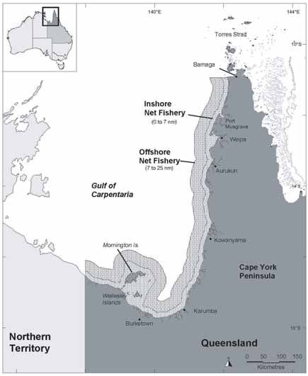
The model is fleet-specific for the Japanese, Australian, and New
Zealand longline fleets, and fishing and movement of fish occurs across
five regions (Fig. 1). Data for the Japanese fleet were available since
1971, while data for the Australian and New Zealand fleets were avail-
able since 1990 and 1991, respectively. The Australian fishery occurred512 Campbell and Dowling—Australian Broadbill Swordfish Fishery
Nauru HB
0
Kiribati
Papua NewGuinea
Tuvalu
Solomon Is.
10
1 4 WF
Vanuatu Fiji
New Caledonia Fiji
20 TO
Australia
MH
Brisbane
2
Norfolk
Is. 30
Sydney New Zealand
Adelaide
CANBERRA
Melbourne 5
3 40
Hobart
140 150 160 170 180
Figure 1. The five regions used to define the spatial structure of the sword-
fish operating model for the southwest Pacific. The light gray areas
indicate exclusive economic zones of individual nation-states.
in areas 1 to 3 while the New Zealand fishery occurred in area 5. Effort
for the Japanese fleet was standardized using a general linear model for
changes in the spatial-temporal distribution of effort, gear configurations
(hooks-per-basket), and the environment (using southern oscillation in-
dex as a proxy) in order to obtain a more appropriate measure of effort
targeted at swordfish (Campbell and Dowling 2003). The Japanese catch
and standardized effort data were also scaled proportionally to accountFisheries Assessment and Management in Data-Limited Situations 513
for catches taken by other foreign fleets operating in the region. Gear
selectivity was assumed to be the same for all fleets, though fishing ef-
ficiencies (catchabilities) were modeled separately by fleet, quarter, and
area to allow for differences and changes in targeting practices. Loss of
catch due to discarding and/or predation was also incorporated in the
model. Campbell and Dowling (2003) further describe the operating
model framework.
Model conditioning
Initial values of R0, the number of recruits in the stock before 1971, and
the parameters of the movement probability matrix were estimated. All
other parameters were input as fixed values for each scenario. Observed
catch by area and quarter was assumed to represent total fishing mor-
tality. For a given R0, the time series of fishing mortality was used with
the modeled natural mortality and recruitment to project the population
forward in time from 1971 to 2001. At the end of this period, features of
the modeled swordfish population were then compared with the historical
catch, catch rate, and size data from the three fisheries and an assumed
level of depletion. This process was repeated until the values of R0 and
the movement parameters that minimized an objective function were
found. At this stage, parameters describing fishery catchabilities were
calculated.
Due to the lack of a stock assessment for swordfish in the southwest
Pacific, the stock status at the end of 2001 remains unknown. For scenario
testing, we considered a range of depletion levels, including upper and
lower extremes as well as an assumed “reference” value:
Low B(2001) = 85% B0
Medium (reference) B(2001) = 70% B0
High B(2001) = 50% B0
These three depletion levels also act as proxies for a high, medium, or low
stock productivity as more productive stocks experience less depletion
for a given level of historical fishing.
Model projections
After being conditioned on the historical data, the model was projected
forward 20 years under each harvest strategy. The fishery dynamics
were controlled by the levels of fishing effort set for each fleet and the
operating model was used to evaluate future conditions of the fishery
and stock.
While the observed catch was used to calculate the fishing mortality
during the conditioning process, during the projection years the catch
needed to be determined from fishing effort. For this purpose, the rela-514 Campbell and Dowling—Australian Broadbill Swordfish Fishery
tionship between nominal effort Enom and fishing mortality F for each fleet
at time t was assumed to be of the form:
F (t ) = Q (t )E nom (t )e
εt −σ 2 /2 (1)
where Q is the catchability and εt is a factor to account for random varia-
tion in catchability [εt ~ N(0;σ2)] . Re-parameterizing Q(t) to have a time-
independent qo and a time-varying Q t component, such that Q(t) = qoQ t,
the above equation can be rewritten in terms of the effective effort Eeff
ε t − σ 2 /2 ε t − σ 2 /2
F (t ) = q oQ t E nom (t )e = q oE eff (t )e (2)
where Eeff = Q tEnom. (3)
The functional form of Q t for each fleet is given in the Appendix. The
parameters describing the fleet specific catchabilities were obtained at
the end of the conditioning phase by minimizing the least-squares dif-
ference between the nominal effort estimated using equation 1 with the
observed effort.
Performance indicators and measures
To describe the performance of the fishery during the projection years,
the following performance indicators were chosen in consultation with
representatives from ETBF stakeholder groups:
Economic
1. Average annual Australian catch (metric tons).
2. Median percentage change in the Australian catch between years.
3. Average percentage of fish in the Australian catch from area 2 that
are greater than 50 kg.
Conservation
1. Final spawning biomass relative to the initial spawning biomass
B0.
2. Probability that the spawning biomass drops below 30% B0.
Collectively these indicators represent three broad management objec-
tives for most fisheries: (1) maximized value of the catch, (2) a sustained
harvest regime, and (3) industrial stability (Walters and Pearse 1996,
Butterworth and Punt 1999). All harvest strategies consequently achieve
some balance among these objectives, and information on trade-offs
among them is needed by decision makers to make informed decisions.Fisheries Assessment and Management in Data-Limited Situations 515
Finally, performance criteria should also be easy for managers and stake-
holders to interpret (Francis and Shotten 1997).
The expected value of each performance indicator under each harvest
strategy was averaged across 100 Monte Carlo simulations.
Fixed effort strategies
In consultation with representatives from ETBF stakeholder groups, a
range of fixed (in the sense that the annual effort for all years was pre-
determined) future effort strategies was identified for consideration.
Hopefully these strategies would bracket future changes in both Austra-
lian and foreign effort and future increases in fishing power, also called
effort creep.
Australian effort
1. Status quo: effort remains at 2001 level of 11.2 million hooks for all
years.
2. Increase in nominal effort over five years to 1.5 × 2001 level (16.8
million hooks) after which time no further increase.
3. Increase in nominal effort over five years to 2.0 × 2001 level (22.4
million hooks) after which time no further increase.
4. Increase in nominal effort over five years to 2.5 × 2001 level (28.0
million hooks) after which time no further increase.
Foreign effort
1. Status quo: effort stays at average level over the last 3 years, 1999-
2001.
2. Increase in effort over five years to 2.0 × status quo level, after which
time no further increase.
Effort creep
1. No increase in effective effort due to effort creep.
2. Increase in effective effort due to effort creep of 2% per annum. Ap-
plied for all years to the Australian fleet and for first five years only
to the foreign fleets (to account for the possible entry of new and
less skilled fishing fleets).
Each of these effort strategies is shown in Figs. 2a and 2b while time
series of total effort for four of the extreme strategies are shown in Fig. 2c.516 Campbell and Dowling—Australian Broadbill Swordfish Fishery
(a) Australian Effort Scenarios
50
Status quo
Status quo + ec
40 16.8 mill (5yrs)
16.8 mill (5yrs) + ec
Millions of Hooks
22.4 mill (5yrs)
30 22.4 mill (5yrs) +ec
28 mill (5yrs)
28 mill (5yrs) +ec
20
10
0
1971 1981 1991 2001 2011 2021
Year
(b) Foreign Effort Scenarios
160
120
Millions of Hooks
80
Status quo
40
Status quo + ec
Double (5yrs)
Double (5yrs) + ec
0
1971 1981 1991 2001 2011 2021
Year
(c) Total Effort Scenarios
200
Status quo
Status quo + ec
160 Maximum
Maximum + ec
Millions of Hooks
120
80
40
0
1971 1981 1991 2001 2011 2021
Year
Figure 2. Time series of annual (a) Australian effort, and (b)
total effort, under different future harvest strate-
gies (ec = effort creep applied).Fisheries Assessment and Management in Data-Limited Situations 517
Table 1. List of future fixed effort harvest strategies used
for evaluation purposes.
Increase in Increase in
Australian foreign
effort effort during Effort
Effort during first first five creep
strategy five years years applied Harvest strategy
1 1 1 No Australian 11.2 m,
foreign sq
2 1 2 Yes Australian 11.2 m+ec,
foreign double+ec
3 1.5 1 No Australian 16.8 m,
foreign sq
4 1.5 1 Yes Australian 16.8 m+ec,
foreign sq
5 1.5 2 Yes Australian 16.8 m+ec,
foreign double+ec
6 2 1 No Australian 22.4 m
foreign sq
7 2 1 Yes Australian 22.4 m+ec,
foreign sq
8 2 2 Yes Australian 22.4 m+ec,
foreign double+ec
9 2.5 1 No Australian 28.0 m,
foreign sq
10 2.5 1 Yes Australian 28.0 m+ec,
foreign sq
11 2.5 2 Yes Australian 28.0 m+ec,
foreign double+ec
Note: sq = status quo, m = million hooks, and ec = effort creep applied.
Table 1 lists the combination of strategies that were selected for evalu-
ation.
Outcomes for each effort strategy were synthesized by taking a
weighted average of the results across each depletion regime. Prob-
abilities of 25, 60, and 15% were assigned to the low, medium, and
high depletion regimes, respectively, guided by the relative size of the
historical catches in relation to swordfish fisheries elsewhere, and the
fit between the historically observed and model predicted catch-at-size
data. To qualitatively assess the performance of each indicator under
each of the effort scenarios, and to assist in presentation of the results to518 Campbell and Dowling—Australian Broadbill Swordfish Fishery
Table 2. Indicative reference levels used to qualitatively assess the
value of each economic and conservation performance indica-
tor.
Management option
Economic Conservation
Qualitative Total Annual Proportion Final Time (%)
rank Australian change in of large spawning biomass
catch catch fish biomass < 30% B0
Excellent ≥ 2.0 > 60%
Very good < 2.0 < 1.0 > 1.0 > 50%
Good < 1.5 < 1.1 > 0.9 > 40% 0%
Moderate < 1.0 < 1.2 > 0.8 > 30% < 10%
Poor ≥ 1.2 > 0.7 > 20% < 20%
Very poor ≤ 0.7 ≤ 20% ≥ 20%
the various ETBF stakeholder groups, the performance of each indicator
was ranked on a qualitative scale between very poor and excellent (Table
2). In assigning ranks, we used 30% B0 as a limit reference point for the
spawning biomass and placed a high value on stabilizing the proportion
of large fish in the catch.
Sensitivity to biological uncertainty
While reproductive studies have been undertaken by Young and Drake
(2002), little other biological work has been undertaken on the swordfish
stock in the southwest Pacific. To overcome this deficiency, a reference
biological scenario was generated by using information on growth, natu-
ral mortality rates, and the stock-recruitment relationship from published
research on swordfish in other oceans.
To examine the sensitivity of MSE outputs to a range of plausible
biological inputs the following alternative scenarios were examined: (1)
steepness in the stock-recruitment relation was changed from 0.9 to 0.65
or 0.4, (2) natural mortality-at-age was multiplied by 1.5, (3) no movement
among areas was permitted, and (4) movement was random (i.e., uniform)
between areas. Relative sensitivity across four different effort strategies
(1, 2, 5, and 11, cf. Table 1) was examined, with all evaluations conducted
under the medium depletion scenario defined earlier.
Harvest strategies involving decision rules
While an examination of stock behavior under fixed harvest strategies
provides information relevant to the choice of an initial TAE for the Aus-You can also read