Seasonal variation and origins of volatile organic compounds observed during 2 years at a western Mediterranean remote background site Ersa, Cape ...
←
→
Page content transcription
If your browser does not render page correctly, please read the page content below
Atmos. Chem. Phys., 21, 1449–1484, 2021
https://doi.org/10.5194/acp-21-1449-2021
© Author(s) 2021. This work is distributed under
the Creative Commons Attribution 4.0 License.

Seasonal variation and origins of volatile organic compounds
observed during 2 years at a western Mediterranean remote
background site (Ersa, Cape Corsica)
Cécile Debevec1 , Stéphane Sauvage1 , Valérie Gros2 , Thérèse Salameh1 , Jean Sciare2,3 , François Dulac2 , and
Nadine Locoge1
1 SAGE  – Département Sciences de l’Atmosphère et Génie de l’Environnement,
IMT Lille Douai, Univ. Lille, 59000 Lille, France
2 Laboratoire des Sciences du Climat et de l’Environnement (LSCE), Unité Mixte CEA-CNRS-UVSQ,

IPSL, Univ. Paris-Saclay, Gif-sur-Yvette, 91190, France
3 Climate and Atmosphere Research Centre, the Cyprus Institute (CyI), Nicosia, 2121, Cyprus

Correspondence: Stéphane Sauvage (stephane.sauvage@imt-lille-douai.fr)
and Cécile Debevec (cecile.debevec@imt-lille-douai.fr)

Received: 16 June 2020 – Discussion started: 8 July 2020
Revised: 5 December 2020 – Accepted: 16 December 2020 – Published: 3 February 2021

Abstract. An original time series of about 300 atmospheric      technique. A PMF five-factor solution was taken on. It in-
measurements of a wide range of volatile organic com-           cludes an anthropogenic factor (which contributed 39 % to
pounds (VOCs) was obtained at a remote Mediterranean            the total concentration of the VOCs selected in the PMF
station on the northern tip of Corsica (Ersa, France) over      analysis) connected to the regional background pollution,
25 months from June 2012 to June 2014. This study presents      three other anthropogenic factors (namely short-lived anthro-
the seasonal variabilities of 35 selected VOCs and their var-   pogenic sources, evaporative sources, and long-lived com-
ious associated sources. The VOC abundance was largely          bustion sources, which together accounted for 57 %) orig-
dominated by oxygenated VOCs (OVOCs) along with pri-            inating from either nearby or more distant emission areas
mary anthropogenic VOCs with a long lifetime in the at-         (such as Italy and south of France), and a local biogenic
mosphere. VOC temporal variations were then examined.           source (4 %). Variations in these main sources impacting
Primarily of local origin, biogenic VOCs exhibited notable      VOC concentrations observed at the Ersa station were also
seasonal and interannual variations, related to temperature     investigated at seasonal and interannual scales. In spring
and solar radiation. Anthropogenic compounds showed in-         and summer, VOC concentrations observed at Ersa were
creased concentrations in winter (JFM months) followed by       the lowest in the 2-year period, despite higher biogenic
a decrease in spring/summer (AMJ/JAS months) and higher         source contributions. During these seasons, anthropogenic
winter concentration levels in 2013 than in 2014 by up          sources advected to Ersa were largely influenced by chem-
to 0.3 µg m−3 in the cases of propane, acetylene and ben-       ical transformations and vertical dispersion phenomena and
zene. OVOC concentrations were generally high in summer-        were mainly of regional origins. During autumn and win-
time, mainly due to secondary anthropogenic/biogenic and        ter, anthropogenic sources showed higher contributions when
primary biogenic sources, whereas their lower concentra-        European air masses were advected to Ersa and could be as-
tions during autumn and winter were potentially more influ-     sociated with potential emission areas located in Italy and
enced by primary/secondary anthropogenic sources. More-         possibly more distant ones in central Europe. Higher VOC
over, an apportionment factorial analysis was applied to a      winter concentrations in 2013 than in 2014 could be related
database comprising a selection of 14 individual or grouped     to contribution variations in anthropogenic sources probably
VOCs by means of the positive matrix factorization (PMF)        governed by their emission strength with external parame-

Published by Copernicus Publications on behalf of the European Geosciences Union.
1450                                        C. Debevec et al.: Seasonal variation and origins of volatile organic compounds

ters, i.e. weaker dispersion phenomena and the pollutant de-       tions in meteorological conditions. Therefore, these elements
pletion. High-frequency observations collected during sev-         underline the necessity of carrying out long-term VOC mea-
eral intensive field campaigns conducted at Ersa during the        surements. Growing efforts are currently being made to con-
three summers 2012–2014 confirmed findings drawn from              duct European background measurements over several sea-
bi-weekly samples of the 2-year period in terms of summer          sons (e.g. Seco et al., 2011), 1 year (such as Helmig et
concentration levels and source apportionment. However,            al., 2008; Legreid et al., 2008) and even several years (Sol-
they also suggested that higher sampling frequency and tem-        berg et al., 1996, 2001, and Tørseth et al., 2012, at sev-
poral resolution, in particular to observe VOC concentration       eral European sites; Hakola et al., 2006, and Hellén et al.,
variations during the daily cycle, would have been necessary       2015, in Scandinavia; Dollard et al., 2007; Grant et al., 2011,
to confirm the deconvolution of the different anthropogenic        and Malley et al., 2015, in the United Kingdom; Borbon
sources identified following the PMF approach. Finally, com-       et al., 2004; Sauvage et al., 2009, and Waked et al., 2016,
parisons of the 25 months of Ersa observations with VOC            in France; Plass-Dülmer et al., 2002, in Germany; Navazo
measurements conducted at 17 other European monitoring             et al., 2008, in the Iberian Peninsula; Lo Vullo et al., 2016
stations highlighted the representativeness of the Ersa station    in Italy). These research studies principally explored the ef-
for monitoring seasonal variations in VOC regional pollu-          fectiveness of emission regulations and links between tro-
tion impacting continental Europe. Nevertheless, VOC win-          pospheric ozone production and VOC concentration levels.
ter concentration levels can significantly vary between sites,     They also assessed seasonal variations and regional distribu-
pointing out spatial variations in anthropogenic source con-       tions of VOC concentrations. Nonetheless, investigations of
tributions. As a result, Ersa concentration variations in winter   principal factors governing temporal and spatial variations
were more representative of VOC regional pollution impact-         in VOC concentration levels in the European background at-
ing central Europe. Moreover, interannual and spatial varia-       mosphere remain scarce. However, the consideration of the
tions in VOC winter concentration levels were significantly        influence of (i) source emission strength variations (built
impacted by synoptic phenomena influencing meteorological          upon a factorial analysis – e.g. Lanz et al., 2009; Lo Vullo
conditions observed in continental Europe, suggesting that         et al., 2016), (ii) long-range transport of pollution (e.g. by
short observation periods may reflect the variability of the       the examination of air-mass trajectories combined with con-
identified parameters under the specific meteorological con-       centrations measured at a study site; Sauvage et al., 2009)
ditions of the study period.                                       and (iii) fluctuations in meteorological conditions (which are
                                                                   prone to dispersing the pollutants over long distances by con-
                                                                   vective and advective transport) can supply relevant informa-
                                                                   tion to deal more in depth with the evaluation of seasonal
1   Introduction                                                   variations and regional distribution of VOC concentrations
                                                                   in the European background atmosphere.
The main trace pollutants in the atmosphere encompass a               Particulate and gaseous pollutants detrimentally affect the
multitude of volatile organic compounds (VOCs), with life-         Mediterranean atmosphere. Accordingly, they are prone to
times varying from minutes to months (e.g. Atkinson, 2000).        increasing aerosol and/or ozone concentration levels in the
Their distribution is principally due to (i) multiple natu-        Mediterranean, regularly higher compared to most regions
ral and anthropogenic sources, which release VOCs directly         of continental Europe, and primarily during summer (Doche
into the atmosphere. At a global scale, natural emissions are      et al., 2014; Nabat et al., 2013; Safieddine et al., 2014).
quantitatively larger than anthropogenic ones (Guenther et         The Mediterranean region is known to be a noteworthy cli-
al., 2000), and the largest natural source is considered to        mate change “hotspot” which is expected to go through se-
be the vegetation (Finlayson-Pitts and Pitts, 2000; Guenther       vere warming and drying in the 21st century (Giorgi, 2006;
et al., 2000, 2006). In urban areas, numerous anthropogenic        Kopf, 2010; Lelieveld et al., 2014). As a consequence, this
sources can abundantly emit various VOCs (Friedrich and            can have serious consequences for the release of VOCs from
Obermeier, 1999). Once in the atmosphere, VOC temporal             biogenic and anthropogenic sources along with their fate in
and spatial variabilities are notably influenced by (ii) mix-      the atmosphere, with uncertain predicted impacts (Colette
ing processes along with (iii) removal processes or chemical       et al., 2012, 2013; Jaidan et al., 2018). Actually, the exam-
transformations (Atkinson, 2000; Atkinson and Arey, 2003).         ination of air composition, concentration levels and trends
Accordingly, with a view to thoroughly characterizing VOC          in the Mediterranean region continues to be challenging,
sources, it is meaningful to examine their chemical compo-         primarily due to the lack of extensive in situ observations.
sition and identify the factors controlling their variations at    Given this context, as part of the multidisciplinary regional
different timescales.                                              research programme MISTRALS (Mediterranean Integrated
   VOC regional distributions change considerably as a result      Studies at Regional and Local Scales; http://mistrals-home.
of various confounding factors, namely the emission strength       org/, last access: 11 October 2020), the project ChArMEx
of numerous potential sources, diverse atmospheric lifetimes       (the Chemistry-Aerosol Mediterranean Experiment; Dulac,
and removal mechanisms, transport processes and fluctua-           2014) aims at assessing the current and future state of the at-

Atmos. Chem. Phys., 21, 1449–1484, 2021                                             https://doi.org/10.5194/acp-21-1449-2021
C. Debevec et al.: Seasonal variation and origins of volatile organic compounds                                                1451

mospheric environment in the Mediterranean along with ex-            vironment (CORSiCA – https://corsica.obs-mip.fr/, last ac-
amining its repercussions for the regional climate, air qual-        cess: 11 October 2020; Lambert et al., 2011) and is located
ity and marine biogeochemistry. Within the framework of              on the highest point of a ridge equipped with windmills (see
ChArMEx, several observation periods were conducted at               the orographic description of the surroundings in Cholakian
the Ersa station, a remote site considered to be representa-         et al., 2018), at an altitude of 533 m above sea level (a.s.l.).
tive of the north-western Mediterranean basin, in order to ex-       Given its position in the north of the 40 km long Cape Corsica
plain variations in VOC concentrations affecting the western         peninsula (Fig. 1), the Mediterranean Sea is clearly visible
Mediterranean atmosphere. Michoud et al. (2017) character-           from the sampling site on the western, northern, and eastern
ized the variations in VOC concentrations observed at Ersa in        sides (2.5–6 km from the sea; see also the figure presented in
summer 2013 (from 15 July to 5 August 2013) by identifying           Michoud et al., 2017). The station was initially set up in or-
and examining their sources.                                         der to monitor and examine pollution advected to Ersa by air
   In this article, we have presented and discussed the factors      masses transported over the Mediterranean and originating
controlling seasonal and interannual variations of a selection       from the Marseille–Fos–Berre region (France; Cachier et al.,
of VOCs observed at the Ersa station over more than 2 years          2005), the Rhone Valley (France), and the Po Valley (Italy;
(from early June 2012 to late June 2014). To this end, this          Royer et al., 2010), namely largely industrialized regions.
study describes (i) the concentration levels of the targeted         The Ersa station is about 30 km north of Bastia (Fig. 1),
VOCs, (ii) their temporal variations at seasonal and interan-        the second largest Corsican city (44121 inhabitants; census
nual scales, (iii) the identification and characteristics of their   2012) and the main harbour. An international airport (Bastia-
main sources by statistical modelling, (iv) the evaluation of        Poretta) is located 16 km further south of Bastia city cen-
their source contributions on seasonal bases, together with          tre. More than 2 million passengers transited in Corsica via
(v) the representativeness of the Ersa station in terms of sea-      Bastia during the tourist season (May–September) in 2013
sonal variations in VOC concentrations impacting continen-           (ORT Corse, 2013). However, as the Cape Corsican penin-
tal Europe.                                                          sula benefits in the south from a mountain range (peaking
                                                                     between 1000 and 1500 m a.s.l.) acting as a natural barrier,
                                                                     the sampling site is therefore not affected by transported pol-
2     Material and methods                                           lution originating from Bastia. Only small rural villages and
                                                                     a small local fishing harbour (Centuri) are found within 5 km
2.1    Study site                                                    of the measurement site. Additionally, the Ersa station is ac-
                                                                     cessible by a dead-end road serving only the windmill site,
Located in the north-western part of the Mediterranean Sea,          surrounded by vegetation made up of Mediterranean maquis,
Corsica is a French territory situated 11 km north of the Sar-       a shrubland biome characteristically consisting of densely
dinian coasts, 90 km east of Tuscany (Italy) and 170 km south        growing evergreen shrubs, and also roamed by a herd of goats
of the French Riviera (France). The fourth largest Mediter-          from a nearby farm. Some forests (78 % of holm oaks, with
ranean island, its land corresponds to an area of 8681 km2           some cork oaks and chestnuts) are also located nearby, thus
encompassed by around 1000 km of coastline (Encyclopædia             ensuring that local anthropogenic pollution does not contam-
Britannica, 2018). Corsica contrasts to other Mediterranean          inate in situ observations. As a result, the Ersa station can be
islands due to the importance of its forest cover (about a fifth     characterized as a remote background Mediterranean site.
of the island).
   Within the framework of the ChArMEx project, an en-               2.2     Experimental set-up
hanced observation period was set up at a ground-based
station in the north of Corsica (Ersa; 42.969◦ N, 9.380◦ E)          2.2.1    VOC measurements
over 25 months, from early June 2012 to late June 2014.
The aim was to provide a high-quality controlled climat-             During a study period of 2 years, non-methane hydrocarbons
ically relevant gas/aerosol database following the recom-            (NMHCs) and OVOCs (carbonyl compounds) were mea-
mendations and criteria of international atmospheric chem-           sured, routinely employing complementary offline methods.
istry networks, i.e. the Aerosol, Clouds and Trace gases             Four-hour-integrated (09:00–13:00 or 12:00–16:00 UTC)
Research Infrastructure (ACTRIS – https://www.actris.eu/,            ambient air samples were collected bi-weekly (every Mon-
last access: 11 October 2020), the European Monitoring and           day and Thursday) into steel canisters and on sorbent car-
Evaluation Program (EMEP – http://www.emep.int/, last ac-            tridges. The inlets were roughly 1.5 m above the roof of a
cess: 11 October 2020; Tørseth et al., 2012), and the Global         container mainly housing trace gas analysers. Table 1 de-
Atmosphere Watch of the World Meteorological Organi-                 scribes VOC measurements set up throughout the observa-
zation (WMO-GAW – http://www.wmo.int/pages/prog/arep/                tion period and Fig. S1 specifies their collection periods.
gaw/gaw_home_en.html, last access: 11 October 2020). The                As generally realized in the EMEP network, 24 C2 –C9
Ersa remote site is part of the Corsican Observatory for Re-         NMHCs were collected into Silcosteel canisters of a volume
search and Studies on Climate and Atmosphere-ocean en-               of 6 L, conforming to the TO-14 technique, which is consid-

https://doi.org/10.5194/acp-21-1449-2021                                              Atmos. Chem. Phys., 21, 1449–1484, 2021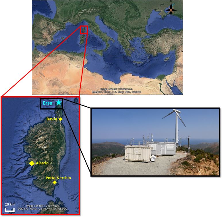
1452                                         C. Debevec et al.: Seasonal variation and origins of volatile organic compounds

Figure 1. Maps of the Mediterranean region and Corsica (source Google Earth) and view of the sampling station. (a) Position of Corsica
in the Mediterranean region. (b) The sampling site and major Corsican agglomerations are displayed as a blue star and yellow diamonds,
respectively. (c) Picture of the sampling site, during the 2-year observation period. Maps provided by Google Earth Pro software (v.7.3.3;
image Landsat/Copernicus; data SIO, NOAA, U.S. Navy, NGA, GEBCO; © Google Earth).

ered adequate for the measurement of many non-polar VOCs               (iv) sampling tests carried out in field conditions and con-
(US-EPA, 1997); 152 air samples were realized with a home-             comitant with in situ measurements (Sauvage et al., 2009).
made device (PRECOV) for sampling air at a steady flow rate               About 150 air samples were gathered using sorbent car-
regulated to 24 mL min−1 by canisters previously placed un-            tridges (63 air samples on multi-sorbent cartridges and 89
der vacuum. NMHC analysis was performed by a gas chro-                 additional ones on 2,4-dinitrophenylhydrazine – DNPH –
matograph coupled with a flame ionization detector (GC-                cartridges), by means of an automatic clean room sampling
FID) within 3 weeks following the sampling. Separation was             system (ACROSS, TERA Environment, Crolles, France).
performed by a system of dual-capillary columns supplied               C1 –C16 VOCs were collected via a 0.635 cm diameter 3 m
with a switching device: the first column was a CP Sil5CB              long PFA line. They were then trapped into one of the
(50 m × 0.25 mm × 1 µm), suitable for the elution of VOCs              two cartridge types: a multi-sorbent one consisting of car-
from six to nine carbon atoms, and the other one was a plot            bopack C (200 mg) and carbopack B (200 mg; marketed un-
Al2 O3 / Na2 SO4 (50 m × 0.32 mm × 5 µm), in order to effec-           der the name of carbotrap 202 by Perkin-Elmer, Welles-
tively elute VOCs from two to five carbon atoms. Four main             ley, Massachusetts, USA) or a Sep-Pak DNPH-Silica one
steps constituted the quality assurance/quality control pro-           (proposed by Waters Corporation, Milford, Massachusetts,
gramme: (i) the implementation of standard operating pro-              USA). These offline techniques are further characterized
cedures, (ii) canister cleaning and certification (blank lev-          in Detournay et al. (2011), and their satisfying use in situ
els < 0.02 ppb), (iii) regular intercomparison exercises and           has already been discussed by Detournay et al. (2013)
                                                                       and Ait-Helal et al. (2014). Succinctly here, the sampling

Atmos. Chem. Phys., 21, 1449–1484, 2021                                                   https://doi.org/10.5194/acp-21-1449-2021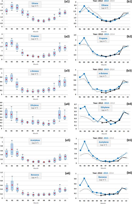
C. Debevec et al.: Seasonal variation and origins of volatile organic compounds                                                1453

Table 1. Technical details of the set-up for VOC measurements during the field campaign from June 2012 to June 2014. Air samples were
collected bi-weekly (every Monday and Thursday) at Ersa from 09:00 to 13:00 UTC (from early November 2012 to late December 2012
and from early November 2013 to late June 2014) or from 12:00 to 16:00 UTC (from early June 2012 to late October 2012 and from early
January 2013 to late October 2013). VOCs are explicitly listed in Sect. S1 of the Supplement.

         Instrument                  Steel canisters –       DNPH cartridges –               Multi-sorbent cartridges –
                                     GC-FID                  chemical desorption             adsorption/thermal
                                                             (acetonitrile) – HPLC-UV        desorption – GC-FID
         Time resolution (min)       240                     240                             240
         Number of samples           152                     91                              63
         Detection limit (µg m−3 )   0.01–0.05               0.02–0.05                       0.01

         Uncertainties U X
                         (X)
                                     25 [7–43]               23 [6–41]                       26 [7–73]
         Mean [min – max] (%)
         Species                     24 C2 –C5 NMHCs         15 C1 –C6 carbonyl compounds    44 C5 –C16 NMHCs
                                                                                             6 C6 –C11 carbonyl compounds
         References                  Sauvage et al. (2009)   Detournay (2011),               Ait-Helal et al. (2014),
                                                             Detournay et al. (2013)         Detournay (2011),
                                                                                             Detournay et al. (2011)

of 44 C5 –C16 NMHCs, comprising alkanes, alkenes, aro-                species were evaluated respecting the ACTRIS-2 guidelines
matic compounds and six monoterpenes, as well as six                  for the uncertainty evaluation (Reimann et al., 2018), consid-
C6 –C11 n-aldehydes, was conducted at a flow rate fixed at            ering precision, detection limit and systematic errors in the
200 mL min−1 and using the multi-sorbent cartridges. These            measurements. Relative uncertainties assessed in this study
latter ones were preliminary prepared by means of a RTA               ranged from 7 % to 43 % for the steel canisters, from 7 % to
oven (French abbreviation for “régénérateur d’adsorbant               73 % for the multi-sorbent cartridges and from 6 % to 41 %
thermique” – manufactured by TERA Environment, Crolles,               for the DNPH cartridges. Finally, the VOC dataset was vali-
France) in order to condition them during 24 h with puri-             dated following the ACTRIS protocol (Reimann et al., 2018).
fied air heated to 250 ◦ C and at a flow rate regulated at               Among the 71 different VOCs monitored at Ersa during
10 mL min−1 . Concomitantly, 15 additional C1 –C8 carbonyl            the observation period, 35 VOCs were finally selected in this
compounds were collected at a flow rate fixed at 1.5 L min−1          study following the methodology described in Sect. S1 of the
using the DNPH cartridges. During the field campaign, sev-            Supplement.
eral ozone scrubbers were successively inserted into the
sampling lines in order to limit any eventual ozonolysis              2.2.2   Ancillary measurements
of the measured VOCs: a MnO2 ozone scrubber was re-
tained for the multi-sorbent cartridges, while KI ozone scrub-        Other trace gases (CO and O3 ) and meteorological parame-
ber was placed upstream of the DNPH cartridges. More-                 ters were ancillary monitored at the Ersa site during the ob-
over, stainless-steel particle filters of 2 µm diameter porosity      servation period. CO was measured from 22 November 2012
(Swagelok) were installed in order to prevent particle sam-           to 16 December 2013 by a cavity ring-down spectroscopy
pling. Then, VOC samples were transferred to the labora-              analyser (G2401; Picarro, Santa Clara, California, USA) at
tory to be analysed within 6 weeks of their collection using          a time resolution of 5 min. O3 was measured from 31 May
a GC-FID (for the multi-adsorbent cartridges) or by a high-           2012 to 26 December 2013 using an ultraviolet absorption
performance liquid chromatograph connected to an ultravio-            analyser (TEI 49i manufactured by Thermo Environmental
let detector (HPLC-UV; for the DNPH cartridges).                      Instruments Inc., Waltham, Massachusetts, USA) at a time
   The reproducibility of each analytical instrument was fre-         resolution of 5 min. Meteorological parameters (temperature,
quently checked by analysing a standard and examining re-             pressure, relative humidity, wind speed, wind direction and
sults by plotting them on a control chart realized for each           total – direct and diffuse – solar radiation) were measured
compound. The VOC detection limit was determined as                   every minute from 8 June to 14 August 2012 and every 5 min
3 times the standard deviation of the blank variation. De-            from 15 August 2012 to 11 July 2014, with a weather sta-
tection limits in this study were all below 0.05 µg m−3 for           tion (CR1000 manufactured by Campbell Scientific Europe,
the steel canisters and the DNPH cartridges and 0.01 µg m−3           Antony, France) placed at approximately 1.5 m above an ad-
for the multi-sorbent cartridges. The uncertainties for each          jacent container roof to the one which housed trace gas in-
                                                                      struments. Note that ancillary trace gas and meteorological

https://doi.org/10.5194/acp-21-1449-2021                                                Atmos. Chem. Phys., 21, 1449–1484, 2021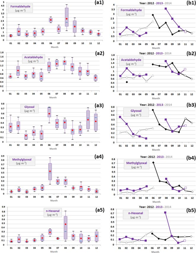
1454 C. Debevec et al.: Seasonal variation and origins of volatile organic compounds
parameter results presented in this study are 4 h averages con- Table 2. Back-trajectory clusters for air masses observed at Ersa
current with VOC sampling periods (see Fig. S1). from June 2012 to June 2014. The transit time (expressed in hours)
corresponds to the time spent since the last anthropogenic contami-
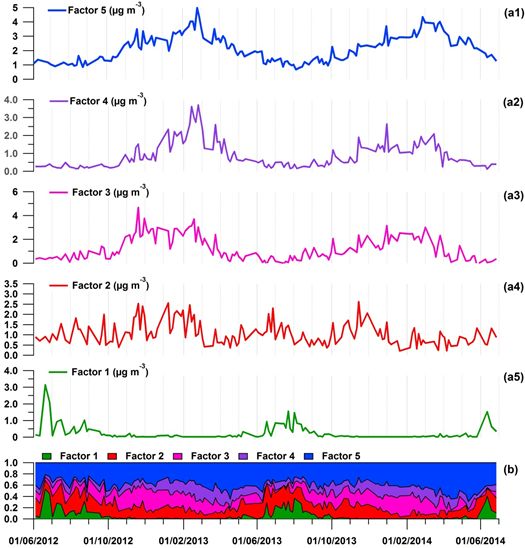
2.3 Identification and contribution of major sources of nation, i.e. since air masses left continental coasts.
VOCs
Clusters Source regions Transit time (h) Occurrence
(wind sectors) Median (%)
In order to characterize NMHC concentrations measured at [min–max]
Ersa with steel canisters (the reasons for this VOC selec-
tion are presented in Sect. S2 of the Supplement), we ap- C1 Marine 48 [18–48] 15
Marine (SW)
portioned them within their sources in this study using the
Short trajectories 48 [39–48] 7
positive matrix factorization approach (PMF; Paatero, 1997; Long trajectories 40 [18–48] 5
Paatero and Tapper, 1994). The PMF mathematical theory
has already been presented in Debevec et al. (2017) and is Marine (SE)
Long trajectories 42 [25–48] 3
therefore mentioned in Sect. S2. We used the PMF version
5.0, an enhanced tool developed by the Environmental Pro- C2 Corsica–Sardinia (S) 0 [0–38] 14
tection Agency (EPA) and including the multilinear engine Short trajectories 2 [0–38] 9
Long trajectories 0 [0–15] 5
program version 2 (ME-2; Paatero, 1999), and followed the
guidance on its use (Norris et al., 2014). Using NMHC in- C3 Europe (NE–E) 6 [2–44] 31
puts composed of 152 atmospheric data points of 14 vari- Short trajectories 23 [4–44] 11
ables (13 single primary NMHCs and another 1 resulting Long trajectories 6 [2–16] 20
from the grouping of C8 aromatic compounds) and follow- C4 France (NW–N) 8 [3–48] 26
ing the methodology presented in Sect. S2, a five-factor PMF Short trajectories 19 [10–48] 6
solution has been selected in this study. Long trajectories 8 [3–19] 20
C5 Spain (W)
2.4 Geographical origins of VOC sources Long trajectories 36 [20–45] 5
2.4.1 Classification of air-mass origins
pathway when they reached the Ersa station, their residence
In order to identify and classify air-mass origins, we anal- time over each potential source region and the length of
ysed back-trajectories calculated by the online version of their trajectories. Additionally, air masses of each cluster
the HYSPLIT Lagrangian model (the Hybrid Single Parti- were subdivided depending on their distance travelled dur-
cle Lagrangian Integrated Trajectory Model developed by ing their 48 h course in order to highlight potential more dis-
the National Oceanic and Atmospheric Administration – tant sources from local ones. This subdivision is also given
NOAA – Air Resources Laboratory; Draxler and Hess, 1998; in Table 2 in order to pinpoint differences in transport times.
Stein et al., 2015) using Ersa as the receptor site (arrival
altitude: 600 m a.s.l.). For each 4 h-atmospheric data point 2.4.2 Identification of potential emission areas
of the field campaign used for the factorial analysis, five
back-trajectories of 48 h were computed using GDAS one- PMF source contributions were coupled with back-
degree resolution meteorological data, in order to follow the trajectories in order to investigate potential emission regions
same methodology as Michoud et al. (2017). The first back- contributing to long-distance pollution transport to the Ersa
trajectory of a set corresponds to the hour when the air sam- site. To achieve this, the concentration field (CF) statistical
pling was initiated (i.e. 09:00 or 12:00 UTC – see Table 1) method established by Seibert et al. (1994) was chosen in the
and the four other ones were calculated every following hour. present study. The CF principle has already been presented in
The time step between each point along the back-trajectories Debevec et al. (2017) and is therefore mentioned in Sect. S3
was fixed at 1 h. of the Supplement.
Then, back-trajectories were visually classified. Having Seventy-two-hour back-trajectories together with meteo-
several back-trajectories per sample allowed us to check rological parameters of interest (i.e. precipitation) were re-
whether air masses transported to the station over 4 h were of trieved from the GDAS meteorological fields with a PC-
the same origin. Samples associated with air masses showing based version of the HYSPLIT Lagrangian model (version
contrasted trajectories (e.g. due to a transitory state between 4 revised in April 2018), following the same methodology as
two different origins) were classified as being of mixed ori- that used for the 48 h back-trajectories previously presented.
gins (9 % of the air masses) and discarded from this study. The arrival time of trajectories at the Ersa station corresponds
Remaining air masses were then manually classified into to the hour when half of the sampling was carried out (i.e.
five trajectory clusters (marine, Corsica–Sardinia, Europe, 11:00 or 14:00 UTC – see Table 1). Note that longer back-
France and Spain – Fig. 2 and Table 2) depending on their trajectories were considered for CF analyses than those for
Atmos. Chem. Phys., 21, 1449–1484, 2021 https://doi.org/10.5194/acp-21-1449-2021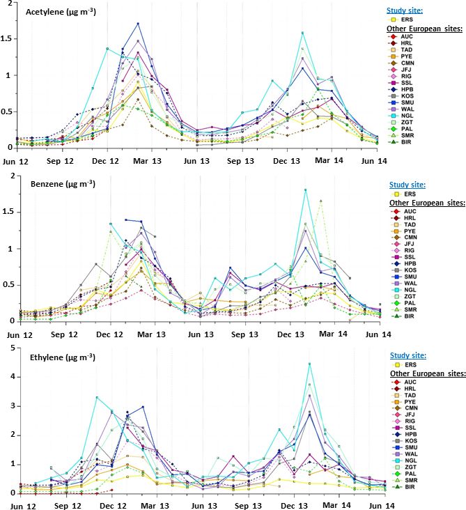
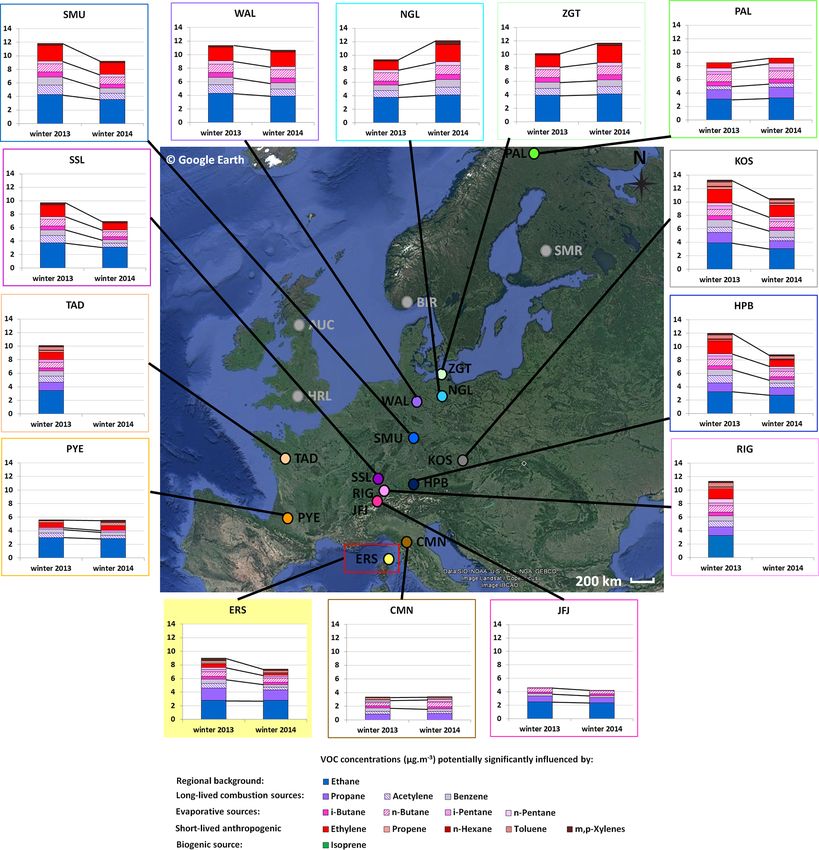
C. Debevec et al.: Seasonal variation and origins of volatile organic compounds                                                         1455

Figure 2. Classification of air masses which impacted the Ersa site during the 2-year observation period as a function of their trajectory.
Back-trajectories simulated with the HYSPLIT Lagrangian model were classified into five clusters: Marine (cluster 1 – wind sectors SW
and SE), Corsica–Sardinia (cluster 2 – S), Europe (cluster 3 – NE–E), France (cluster 4 – NW–N) and Spain (cluster 5 – W). These five
clusters were illustrated by example maps with five trajectories (interval of 1 h between each, time of arrival indicated by different colours
of trajectory, the Ersa station represented by a black star) for 5 d that are representative of an isolated cluster. Finally, areas covered by
back-trajectories of each cluster are also indicated. Maps provided by Google Earth Pro software (v.7.3.3; image Landsat/Copernicus; data
SIO, NOAA, U.S. Navy, NGA, GEBCO; © Google Earth).

air-mass origin classification (Sect. 2.4.1), in order to be in          the possible influence of elevated concentrations, which may
the same conditions as Michoud et al. (2017) and hence to                be observed during occasional episodes (e.g. Bressi et al.,
have comparative results between the two Ersa VOC studies.               2014; Waked et al., 2014, 2018), on cells with a low number
   CF analyses applied to VOC source contributions were                  of trajectory points. We initially tried to apply this weighing
carried out by means of the ZeFir tool (version 3.70; Petit              function in this study. Exploratory tests revealed that CF re-
et al., 2017). Back-trajectories were shortened (i.e. the Ze-            sults with the empirical weighing function only highlighted
Fir tool considered shorter back-trajectories than 72 h) when            local contributions, given the number of air masses of this
precipitation higher than 0.1 mm was encountered along the               study. The farther a cell was from the Ersa station, the lower
trajectory (Bressi et al., 2014). As done by Michoud et                  was its corresponding nij value (number of points of the to-
al. (2017), back-trajectories have also been shortened when              tal number of back-trajectories contained in the ij th grid cell,
air-mass altitudes exceeded 1500 m a.s.l. in order to discard            Sect. S3 of the Supplement) and the more the weighing func-
biases related to the significant dilution impacting air masses          tion tended toward downweighting the results related to this
reaching the free troposphere. A better statistical significance         cell. Therefore, CF results discussed in this study were real-
of the CF results is commonly considered for grid cells with             ized without weighing, and these limitations should be taken
a high number of crossing trajectory points. As a result, some           into account when examining CF analyses, which are hence
studies applied an empirical weighing function so as to limit            considered to be indicative information.

https://doi.org/10.5194/acp-21-1449-2021                                                    Atmos. Chem. Phys., 21, 1449–1484, 2021
1456                                         C. Debevec et al.: Seasonal variation and origins of volatile organic compounds

   Finally, the spatial coverage of grid cells was set from         in 2012 than in 2013 and 2014 (mean relative humidities
(9◦ W, 32◦ N) to (27◦ E, 54◦ N), with a grid resolution of          of 57 ± 15 %, 77 ± 16 % and 67 ± 33 % in 2012, 2013 and
0.3◦ × 0.3◦ . Allocated contributions were smoothed follow-         2014, respectively). The wind speed did not show a clear sea-
ing a factor (corresponding to the strength of a Gaussian fil-      sonal variation over the 2 years studied. Wind speeds were
ter) set to 5 to take into account the uncertainties in the back-   slightly higher in April and May, which could induce higher
trajectory path (Charron et al., 2000).                             dispersion of air pollutants and favour their advection to the
                                                                    Ersa station by the most distant sources.

3     Results                                                       3.2   Air-mass origins

3.1    Meteorological conditions                                    Occurrences of air-mass origins which influenced Ersa
                                                                    throughout the observation period are indicated in Table 2.
Monthly variations in meteorological parameters are de-             The Ersa station was predominantly influenced by continen-
picted in Fig. 3. As the field measurement period covered           tal air masses coming from Europe (corresponding to clus-
2 years (i.e. from June 2012 to June 2014), their interannual       ter 3, 31 %), France (cluster 4, 26 %), Corsica–Sardinia (clus-
variations are also shown in Fig. 3b.                               ter 2, 14 %) and Spain (cluster 5, 5 %) and to a lesser ex-
   Air temperatures showed typical seasonal variations, i.e.        tent by air masses predominantly of marine origin (cluster 1,
the highest recorded in summer (i.e. the months of July             15 %). Each of these five clusters is mostly associated with a
to September) and the lowest in winter (i.e. the months             particular trajectory sector (e.g. south for air masses originat-
of January to March). They were globally in the range of            ing from Corsica and/or Sardinia; see Fig. 2) and is defined
normal values over the period 1981–2010 determined by               by a different transit time from continental coasts. Accord-
Météo-France (the French national meteorological service;           ing to Michoud et al. (2017), transit time can be viewed as
normal values correspond to minimal and maximal mean                an indicator of the last time when an air mass could have
values determined for Bastia and are available for con-             been enriched in anthropogenic sources (Table 2). Continen-
sultation at http://www.meteofrance.fr/climat-passe-et-futur/       tal air masses spent less time over the sea than marine ones.
climathd, last access: 11 October 2020). Moreover, June tem-        Transit times of continental air masses over the sea differed
peratures were colder in 2013 than in 2012 and 2014 (mean           depending on how they were categorized. Air masses orig-
temperatures of 24.7 ± 5.8, 19.4 ± 4.1 and 22.5 ± 5.4 ◦ C in        inating from Corsica–Sardinia, France and Europe spent 0–
2012, 2013 and 2014, respectively), which could have influ-         8 h (median values – Table 2) above the sea before reaching
enced biogenic emissions. Winter temperatures were colder           the Ersa station, while the air masses originating from Spain
in 2013 than in 2014 (mean temperatures of 7.0 ± 4.1 and            spent about 36 h. These contrasting transit times may denote
9.7 ± 1.5 ◦ C in 2013 and 2014, respectively). This finding         both distinctive atmospheric processing times for air masses
could be explained by different winter climatic events which        and different oceanic source influences on VOC concentra-
affected a large part of continental Europe in 2013 and 2014.       tions observed at the Ersa station.
On the one hand, the European winter was particularly harsh            European and French air masses showed lower transit
in 2013, caused by changes in air-flux orientation originally       times over the sea (median values of 6 and 8 h, respectively;
due to the sudden stratospheric warming of the stratospheric        Table 2) when their trajectories were categorized as long,
polar vortex (Coy and Pawson, 2015). On the other hand,             compared to short ones (23 and 19 h, respectively). These
most of the western European countries experienced a mild           findings are based on the fact that an air-mass trajectory clas-
winter in 2014 characterized by its lack of cold outbreaks and      sified as short has a closer distance between two of its suc-
nights and caused by an anomalous atmospheric circulation           cessive trajectory points compared to another one classified
(Rasmijn et al., 2016; Van Oldenborgh et al., 2015; Watson          as long. Due to the Ersa location in the Mediterranean Sea,
et al., 2016).                                                      air masses with trajectories categorized as long spent longer
   Solar radiation followed typical seasonal variations, with       periods above the sea before reaching the Ersa site. Note that
the highest recorded from May to August and the lowest              European and French air masses were more frequently char-
in December and January. Spring (i.e. the months of April           acterized by long trajectories (accounting for 20 % of the
to June) solar radiations were higher in 2014 than in 2013          air masses observed at Ersa during the studied period, for
(average values of 371 ± 157 and 478 ± 153 W m−2 in 2013            each) than short ones (11 % and 6 %, respectively). More-
and 2014, respectively). Summer solar radiations were higher        over, marine air masses with short and long trajectories both
in 2013 than in 2012 (average values of 332 ± 164 and               showed long transit times (median values of 40–48 h – Ta-
395 ± 128 W m−2 in 2012 and 2013, respectively). These              ble 2). Corsican–Sardinian air masses were only character-
solar radiation variations may have affected biogenic VOC           ized by long trajectories.
(BVOC) emissions and photochemical reactions.
   Relative humidity followed opposite seasonal variations
in temperature and solar radiation. Air in June was drier

Atmos. Chem. Phys., 21, 1449–1484, 2021                                               https://doi.org/10.5194/acp-21-1449-2021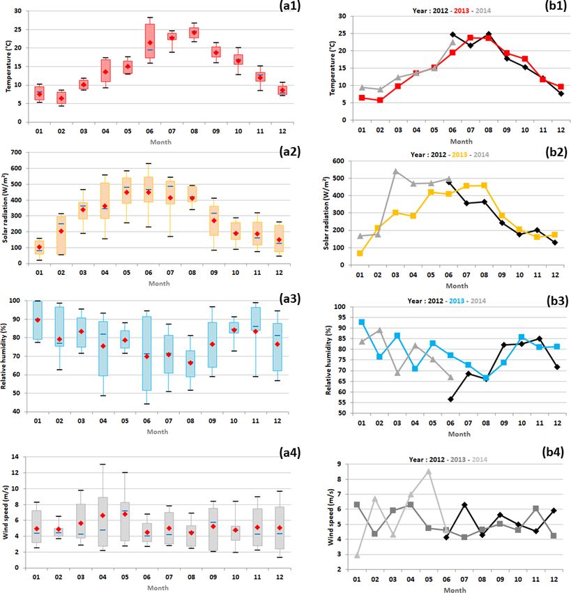
C. Debevec et al.: Seasonal variation and origins of volatile organic compounds                                                        1457

Figure 3. (a) Monthly variations in meteorological parameters (temperature expressed in ◦ C, global solar radiation in W m−2 , relative
humidity in % and wind speed in m s−1 ) represented by box plots; the blue solid line, the red marker, and the box represent the median,
the mean, and the interquartile range of the values, respectively. The bottom and top of the box depict the first and third quartiles and the
ends of the whiskers correspond to the first and ninth deciles. (b) Their monthly average concentrations as a function of the year. Note that
meteorological parameter data used in this study were restricted to periods when VOC measurements were realized.

https://doi.org/10.5194/acp-21-1449-2021                                                   Atmos. Chem. Phys., 21, 1449–1484, 2021
1458 C. Debevec et al.: Seasonal variation and origins of volatile organic compounds
3.3 VOC mixing ratios ported the representativeness of the 2-year observation pe-
riod with regard to its summer concentration levels.
Statistical results of concentrations of the 35 VOCs selected
in this study (see Sect. S1 in the Supplement) are summarized 3.4.1 Biogenic VOCs
in Table 3. Their average concentration levels as a function
of the measurement sampling time (09:00–13:00 or 12:00– Concentration variations of three selected BVOCs, iso-
16:00 UTC) are also indicated in Table S1. These VOCs prene, α-pinene and camphene, were analysed at different
were organized into three principal categories: biogenic, an- timescales (monthly/interannual variations; Fig. 4). These
thropogenic, and oxygenated VOCs (5, 16 and 14 targeted BVOCs exhibited high concentrations from June to August
species, respectively; Table 3). Isoprene and four monoter- consistently with temperature and solar radiation variations
penes were classified into BVOCs, while the other primary (see Sect. 3.1). Indeed, throughout the summer 2013 obser-
hydrocarbons (alkanes, alkenes, alkynes and aromatic com- vation period, Michoud et al. (2017) and Kalogridis (2014)
pounds) were included in anthropogenic NMHCs, since their observed that emissions of isoprene and the sum of monoter-
emissions are especially in connection with human activi- penes were mainly governed by temperature and solar radi-
ties. OVOCs have been presented separately, as these com- ation, supported both by the diurnal variations in their con-
pounds come from both biogenic and anthropogenic (pri- centrations (Geron et al., 2000a, b; Guenther et al., 2000)
mary and secondary) sources. OVOCs were the most abun- and their correlations with environmental parameters. Ad-
dant, accounting for 65 % of the total concentration of the 35 ditionally, significant concentrations of α-pinene were no-
VOCs selected in this study. They were mainly composed of ticed from September to November (Fig. 4), while isoprene
acetone (contribution of 51 % to the OVOC cumulative con- concentrations were close to the detection limit and tem-
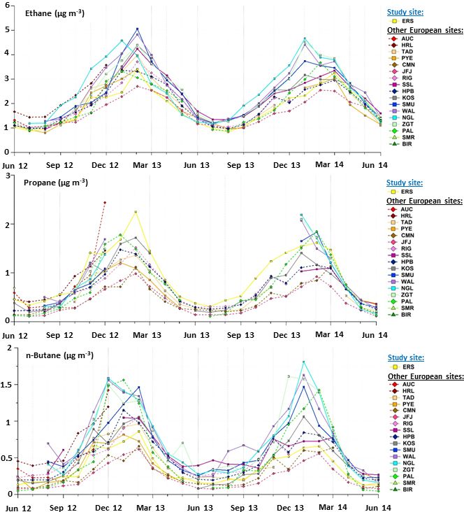
centration). Anthropogenic NMHCs also contributed signifi- perature and solar radiation were decreasing. However, so-
cantly (26 %) to the total VOC concentration and principally lar radiation decreased much faster than temperature dur-
consisted of ethane and propane (which represented 34 % and ing these months (Fig. 3), which could suggest that addi-
17 % of the anthropogenic NMHC cumulative concentration, tional emissions (Laothawornkitkul et al., 2009), dependent
respectively) as well as n-butane (7 %). The high contribution only on temperature contrary to those prevailing in sum-
of species which generally have the longest lifetimes in the mer, have influenced α-pinene concentrations during these
atmosphere (see Sect. 3.5) is consistent with the remote lo- months. Ozone concentrations, lower in autumn (i.e. the
cation of the Ersa site and is in agreement with Michoud et months of October to December) than in summer (O3 con-
al. (2017). BVOCs contributed little to the total VOC concen- centration variations are depicted in Fig. S2 of the Supple-
tration (9 % on annual average, 13 % in summer). They were ment), also pointed out a weaker degradation of α-pinene in
mainly composed of isoprene and α-pinene (contributions of autumn.
44 % and 32 % to the BVOC mass, respectively). These com- Biogenic compounds showed significant interannual vari-
pounds are among the major BVOCs in terms of emission in- ations over the study period, linked to temperature and solar
tensity for the Mediterranean vegetation (Owen et al., 2001) radiation variations. Higher June concentrations of isoprene
and accounted for half of isoprenoid concentrations recorded and α-pinene were noticed in 2012 (average concentrations
during the intensive field campaign conducted at Ersa in sum- of 1.0 ± 1.1 and 2.6 ± 1.4 µg m−3 for isoprene and α-pinene,
mer 2013 (Debevec et al., 2018; Kalogridis, 2014). By con- respectively) and 2014 (0.7 ± 0.5 and 0.2 µg m−3 ) than in
trast, a larger α-terpinene contribution was noticed during the 2013 (0.2 ± 0.2 and < 0.1 µg m−3 ). Higher June concentra-
summer 2013 intensive field campaign than the 2-year obser- tions of camphene (and α-terpinene; not shown) were also
vation period. Note that speciated monoterpenes were mea- noticed in 2014 than in 2013 (Fig. 4). These concentration
sured differently during the summer 2013 field campaign by levels may be related to the fact that temperature and solar
means of an automatic analyser (see Sect. S4 in the Supple- radiation were more favourable to enhancing June biogenic
ment). emissions in 2012 and 2014 than in 2013 (Sect 3.1). Due
to air relative humidity values observed in June (Sect. 3.1),
we cannot rule out that an increase in BVOC concentrations
3.4 VOC variability may be linked to a transient modification of BVOC emis-
sions induced by drought stress (Ferracci et al., 2020; Loreto
Monthly and interannual variations of primary (anthro- and Schnitzler, 2010; Niinemets et al., 2004). Moreover,
pogenic and biogenic) NMHCs along with OVOCs selected isoprene and α-pinene concentrations in July and August
in this study (Sect. S1) are discussed in this section. Sea- were higher in 2013 (average concentrations of 0.5 ± 0.3 and
sonal VOC concentration levels are indicated in Table 4. Note 1.1 ± 0.4 µg m−3 for isoprene and α-pinene, respectively)
that the results of comparison between the VOC monitor- than in 2012 (0.3 ± 0.2 and 0.6 ± 0.3 µg m−3 ). High concen-
ing measurements investigated in this study and concurrent trations of camphene and α-terpinene were also noticed in
field campaign measurements performed during the summers August 2013 (0.2 ± 0.1 and 0.3 ± 0.3 µg m−3 , respectively;
2012–2014 (presented in Sect. S4 of the Supplement) sup- Fig. 4). Solar radiations were lower in July and August 2012,
Atmos. Chem. Phys., 21, 1449–1484, 2021 https://doi.org/10.5194/acp-21-1449-2021C. Debevec et al.: Seasonal variation and origins of volatile organic compounds 1459
Table 3. Statistics (µg m−3 ), standard deviations (σ – µg m−3 ), detection limits (DL – µg m−3 ) and relative uncertainties (Unc. – %) of
selected VOC concentrations measured at the site from June 2012 to June 2014.
Species Min 25 % 50 % Mean 75 % Max σ DL Unc.
BVOCs Isoprene 0.01 0.01 0.04 0.16 0.16 2.28 0.31 0.03 32
α-Pinene < 0.01 0.03 0.10 0.38 0.57 3.61 0.61 0.01 40
Camphene < 0.01 0.01 0.05 0.12 0.13 0.78 0.17 0.01 73
α-Terpinene < 0.01 < 0.01 < 0.01 0.06 0.05 0.88 0.15 0.01 47
Limonene < 0.01 < 0.01 0.03 0.19 0.36 1.73 0.30 0.01 45
Anthropogenic Ethane 0.57 1.13 1.85 1.86 2.46 4.28 0.81 0.01 7
NMHCs Propane 0.18 0.44 0.77 0.94 1.41 2.60 0.61 0.02 11
i-Butane 0.01 0.09 0.17 0.24 0.35 1.02 0.19 0.02 22
n-Butane 0.05 0.16 0.26 0.37 0.57 1.09 0.26 0.02 13
i-Pentane 0.06 0.15 0.22 0.25 0.31 0.90 0.14 0.03 25
n-Pentane 0.02 0.09 0.18 0.20 0.27 0.80 0.13 0.03 33
n-Hexane 0.02 0.04 0.07 0.08 0.10 0.27 0.05 0.04 43
Ethylene 0.09 0.19 0.28 0.32 0.39 0.87 0.17 0.01 14
Propene 0.01 0.04 0.06 0.07 0.09 0.17 0.03 0.02 40
Acetylene 0.03 0.09 0.18 0.26 0.36 1.23 0.23 0.01 12
Benzene 0.07 0.16 0.26 0.31 0.39 1.11 0.19 0.03 25
Toluene 0.04 0.15 0.23 0.28 0.34 0.84 0.17 0.04 26
Ethylbenzene 0.02 0.02 0.02 0.04 0.05 0.15 0.03 0.04 50
m,p-Xylenes 0.02 0.07 0.10 0.12 0.14 0.41 0.08 0.04 45
o-Xylene 0.02 0.02 0.06 0.07 0.10 0.32 0.06 0.04 44
OVOCs Formaldehyde 0.28 0.68 1.17 1.53 1.89 6.30 1.24 0.03 7
Acetaldehyde 0.40 0.67 0.83 0.96 1.23 2.87 0.41 0.03 22
i,n-Butanals < 0.01 0.10 0.15 0.26 0.23 5.15 0.56 0.03 20
n-Hexanal < 0.01 0.08 0.13 0.22 0.24 1.83 0.27 0.03 12
Benzaldehyde < 0.01 0.06 0.13 0.15 0.22 0.60 0.12 0.04 21
n-Octanal < 0.01 0.01 0.05 0.05 0.11 1.25 0.20 0.01 39
n-Nonanal < 0.01 0.07 0.21 0.21 0.37 1.42 0.31 0.01 33
n-Decanal < 0.01 0.04 0.16 0.16 0.31 1.19 0.26 0.01 33
n-Undecanal < 0.01 0.04 0.05 0.05 0.08 0.33 0.06 0.01 39
Glyoxal < 0.01 0.04 0.06 0.07 0.11 0.25 0.05 0.02 27
Methylglyoxal < 0.01 0.07 0.11 0.16 0.19 0.95 0.15 0.04 23
Acetone 1.50 2.46 3.57 4.31 4.98 16.49 2.64 0.03 6
MEK 0.18 0.27 0.33 0.36 0.45 0.90 0.14 0.03 10
temperatures were slightly lower in July 2012 and mean wind 3.4.2 Anthropogenic VOCs
speed was slightly higher in July 2012 (Fig. 3). These mete-
orological conditions may have affected biogenic emissions Variations of a selection of NMHCs are depicted in Fig. 5.
and have favoured their dispersion and their dilution by ma- These compounds illustrate contrasted reactivity, based on
rine air masses, owing to the position of the Ersa station their atmospheric lifetimes (estimated according to their pho-
(Sect. 2.1). tochemical reaction rates with OH radicals defined in Atkin-
Note that the interpretation of interannual variations in son, 1990, and Atkinson and Arey, 2003). Despite lifetimes
BVOC measurements is based on a limited number of sam- in the atmosphere ranging from a few hours to some days,
pling days during the study period and different collection all selected NMHCs were characterized by similar seasonal
times (Table 1 and Sect. 2.2.1). It should therefore be consid- variations, with an increasing winter trend followed by a de-
ered cautiously, given variable day-to-day and strong diurnal crease in spring/summer (Fig. 5 and Table 4), with the excep-
BVOC concentration variations which were observed during tion of n-hexane, propene and C8 aromatics (which were the
the summer 2013 observation period (Kalogridis, 2014). most reactive species of the NMHCs selected in this study
and had the lowest concentrations; Tables 3 and 4). NMHC
concentrations were higher in winter than in summer, up to
5 times higher in the case of acetylene (Table 4). Note that
ethane concentration levels were relatively important dur-
https://doi.org/10.5194/acp-21-1449-2021 Atmos. Chem. Phys., 21, 1449–1484, 20211460 C. Debevec et al.: Seasonal variation and origins of volatile organic compounds
Table 4. Average VOC seasonal concentrations (±1σ ; µg m−3 ).
Species Winter Spring Summer Autumn
BVOCs Isoprene 0.1 ± 0.1 0.2 ± 0.5 0.3 ± 0.3 0.1 ± 0.1
α-Pinene 0.1 ± 0.1 0.3 ± 0.9 0.7 ± 0.5 0.5 ± 0.5
Camphene 0.1 ± 0.1 0.1 ± 0.1 0.1 ± 0.1 0.1 ± 0.1
α-Terpinene 0.1 ± 0.1 0.1 ± 0.1 0.3 ± 0.3 0.1 ± 0.1
Limonene 0.1 ± 0.1 0.1 ± 0.4 0.4 ± 0.2 0.3 ± 0.3
Anthropogenic Ethane 2.9 ± 0.5 1.8 ± 0.6 1.0 ± 0.2 1.9 ± 0.5
NMHCs Propane 1.7 ± 0.4 0.6 ± 0.2 0.4 ± 0.2 1.2 ± 0.5
i-Butane 0.4 ± 0.1 0.1 ± 0.1 0.1 ± 0.1 0.4 ± 0.2
n-Butane 0.7 ± 0.2 0.2 ± 0.1 0.2 ± 0.1 0.5 ± 0.2
i-Pentane 0.3 ± 0.1 0.2 ± 0.1 0.2 ± 0.1 0.3 ± 0.1
n-Pentane 0.2 ± 0.1 0.2 ± 0.2 0.2 ± 0.1 0.3 ± 0.1
n-Hexane 0.1 ± 0.1 0.1 ± 0.1 0.1 ± 0.1 0.1 ± 0.1
Ethylene 0.5 ± 0.2 0.2 ± 0.1 0.2 ± 0.1 0.4 ± 0.5
Propene 0.1 ± 0.1 0.1 ± 0.1 0.1 ± 0.1 0.1 ± 0.1
Acetylene 0.5 ± 0.3 0.2 ± 0.1 0.1 ± 0.1 0.3 ± 0.1
Benzene 0.5 ± 0.2 0.2 ± 0.1 0.2 ± 0.1 0.4 ± 0.1
Toluene 0.3 ± 0.2 0.2 ± 0.1 0.2 ± 0.1 0.3 ± 0.2
C8-aromatics 0.2 ± 0.2 0.2 ± 0.2 0.2 ± 0.1 0.2 ± 0.2
OVOCs Formaldehyde 0.8 ± 0.5 1.3 ± 0.8 2.3 ± 1.3 1.1 ± 0.4
Acetaldehyde 0.8 ± 0.3 0.8 ± 0.3 1.3 ± 0.4 0.8 ± 0.3
i,n-Butanals 0.1 ± 0.1 0.1 ± 0.1 0.5 ± 1.0 0.1 ± 0.1
n-Hexanal 0.1 ± 0.1 0.2 ± 0.1 0.4 ± 0.4 0.2 ± 0.1
Benzaldehyde 0.2 ± 0.1 0.1 ± 0.2 0.2 ± 0.1 0.1 ± 0.1
n-Octanal 0.1 ± 0.1 0.1 ± 0.1 0.2 ± 0.4 0.1 ± 0.1
n-Nonanal 0.3 ± 0.4 0.4 ± 0.4 0.1 ± 0.2 0.3 ± 0.2
n-Decanal 0.3 ± 0.3 0.3 ± 0.3 0.1 ± 0.1 0.3 ± 0.2
n-Undecanal 0.1 ± 0.1 0.1 ± 0.1 0.1 ± 0.1 0.1 ± 0.1
Glyoxal 0.1 ± 0.1 0.1 ± 0.1 0.1 ± 0.1 0.1 ± 0.1
Methylglyoxal 0.1 ± 0.1 0.2 ± 0.2 0.3 ± 0.2 0.1 ± 0.1
Acetone 2.7 ± 1.2 3.8 ± 1.4 5.8 ± 1.8 3.7 ± 1.8
MEK 0.4 ± 0.1 0.3 ± 0.1 0.4 ± 0.2 0.4 ± 0.1
ing summer (mean concentration of 1.0 ± 0.2 µg m−3 ), while other hand, acetone and methyl ethyl ketone (MEK) have the
other NMHCs showed concentrations below 0.4 µg m−3 . longest atmospheric lifetime among the OVOCs selected in
NMHCs exhibited different concentration levels during this study, and hence they can also result from distant sources
the two studied winter periods (Fig. 5). Mean winter NMHC and/or be formed within emission-enriched air masses ad-
concentrations were higher in 2013 than in 2014 by up vected to the Ersa station.
to 0.3 µg m−3 in the cases of propane, acetylene and ben- Firstly, formaldehyde, methylglyoxal and n-hexanal have
zene (relative differences of 15 %, 42 % and 42 %, respec- shown similar seasonal variations (Fig. 6), with high sum-
tively). These compounds and ethane had the longest life- mer and spring concentrations (Table 4), suggesting an im-
times among those selected in this study. However, ethane portant contribution of primary/secondary biogenic sources
concentrations recorded at Ersa did not show any interannual to their concentrations. Fu et al. (2008) found that the largest
variation over the study period (Fig. 5). global sources for methylglyoxal were isoprene and to a
lesser extent acetone. Besides photochemical production, n-
3.4.3 Oxygenated VOCs hexanal and formaldehyde can be notably emitted by many
plant species (Guenther et al., 2000; Kesselmeier and Staudt,
Variations of selected OVOCs, illustrating contrasted reac- 1999; Wildt et al., 2003). Interannual variations in formalde-
tivity (following the same methodology as that applied to hyde, methylglyoxal and n-hexanal summer concentrations
NMHCs; Sect. 3.4.2), are presented in Fig. 6. Formaldehyde, confirmed their links with biogenic sources. For instance,
acetaldehyde, glyoxal, methylglyoxal and C6 –C11 aldehy- the highest concentrations of methylglyoxal were observed
des have relatively short lifetimes into the atmosphere, and in June 2012 (average concentration of 0.7 µg m−3 ), simi-
hence they can result from relatively close sources. On the
Atmos. Chem. Phys., 21, 1449–1484, 2021 https://doi.org/10.5194/acp-21-1449-2021C. Debevec et al.: Seasonal variation and origins of volatile organic compounds 1461 Figure 4. (a) Monthly variations in a selection of biogenic VOC concentrations (expressed in µg m−3 ) represented by box plots; the blue solid line, the red marker, and the box represent the median, the mean, and the interquartile range of the values, respectively. The bottom and top of the box depict the first and third quartiles and the ends of the whiskers correspond to the first and ninth deciles. (b) Their monthly average concentrations as a function of the year; full markers indicate months when VOC samples were collected from 12:00 to 16:00 UTC and empty markers those when VOC samples were collected from 09:00 to 13:00 UTC. larly to isoprene (Sect. 3.4.1). Monthly concentrations of n- and Schade, 2000; Schade and Goldstein, 2006). Acetone can hexanal peaked at 0.7 µg m−3 in August 2013, in agreement also result from the oxidation of various VOCs (Goldstein with monoterpenes, especially camphene and α-terpinene and Schade, 2000; Jacob et al., 2002; Singh et al., 2004), (Sect. 3.4.1). Formaldehyde showed high concentrations in and roughly half of its concentrations measured at diverse ur- both June 2012 and August 2013 (2.9 and 3.6 µg m−3 , re- ban or rural sites have been assigned to regional background spectively). pollution by several studies (e.g. Debevec et al., 2017; de Acetaldehyde and acetone have shown an increase in Gouw et al., 2005; Legreid et al., 2007; with regional contri- their concentrations more marked in summer than in winter butions at a scale of hundreds of kilometres). Additionally, (Fig. 6), suggesting they were probably mainly of both sec- acetaldehyde and acetone concentration variations in win- ondary (anthropogenic/biogenic) and primary biogenic ori- ter (e.g. mean February concentration in 2013 was 0.5 and gins. Acetaldehyde is known to be mainly produced through 2.4 µg m−3 higher than in 2014, respectively) also pinpointed the chemical transformation of anthropogenic and biogenic primary/secondary anthropogenic origins (Sect. 3.4.2). VOCs (Rottenberger et al., 2004; Schade and Goldstein, Glyoxal and MEK showed an increase in their concen- 2001; Seco et al., 2007; Wolfe et al., 2016), particularly in trations in both summer and winter (Fig. 6 and Table 4), clean and remote areas. Acetaldehyde can also be released by suggesting they were probably produced by several biogenic plants (Jardine et al., 2008; Rottenberger et al., 2008; Win- and anthropogenic sources. Glyoxal increases were in simi- ters et al., 2009). Acetone emissions are thought to be glob- lar proportions (Fig. 6 and Table 4), while the MEK increase ally of biogenic rather than anthropogenic origin (Goldstein in winter was more marked than in summer, which may https://doi.org/10.5194/acp-21-1449-2021 Atmos. Chem. Phys., 21, 1449–1484, 2021
1462                                            C. Debevec et al.: Seasonal variation and origins of volatile organic compounds

Figure 5. (a) Monthly variations in a selection of anthropogenic VOC concentrations (expressed in µg m−3 ) represented by box plots; the
blue solid line, the red marker, and the box represent the median, the mean, and the interquartile range of the values, respectively. The bottom
and top of the box depict the first and third quartiles and the ends of the whiskers correspond to the first and ninth deciles. (b) Their monthly
average concentrations as a function of the year; full markers indicate months when VOC samples were collected from 12:00 to 16:00 UTC
and empty markers those when VOC samples were collected from 09:00 to 13:00 UTC.

Atmos. Chem. Phys., 21, 1449–1484, 2021                                                       https://doi.org/10.5194/acp-21-1449-2021
You can also read