Marine terraces of the last interglacial period along the Pacific coast of South America (1 N-40 S)
←
→
Page content transcription
If your browser does not render page correctly, please read the page content below
Earth Syst. Sci. Data, 13, 2487–2513, 2021
https://doi.org/10.5194/essd-13-2487-2021
© Author(s) 2021. This work is distributed under
the Creative Commons Attribution 4.0 License.

         Marine terraces of the last interglacial period along the
              Pacific coast of South America (1◦ N–40◦ S)
              Roland Freisleben1 , Julius Jara-Muñoz1 , Daniel Melnick2,3 , José Miguel Martínez2,3 , and
                                                Manfred R. Strecker1
                      1 Institut
                               für Geowissenschaften, Universität Potsdam, 14476 Potsdam, Germany
               2 Instituto
                         de Ciencias de la Tierra, TAQUACH, Universidad Austral de Chile, Valdivia, Chile
                     3 Millennium Nucleus the Seismic Cycle along Subduction Zones, Valdivia, Chile

                              Correspondence: Roland Freisleben (freisleb@uni-potsdam.de)

                               Received: 11 December 2020 – Discussion started: 18 December 2020
                              Revised: 2 April 2021 – Accepted: 7 April 2021 – Published: 3 June 2021

      Abstract. Tectonically active coasts are dynamic environments characterized by the presence of multiple ma-
      rine terraces formed by the combined effects of wave erosion, tectonic uplift, and sea-level oscillations at glacial-
      cycle timescales. Well-preserved erosional terraces from the last interglacial sea-level highstand are ideal marker
      horizons for reconstructing past sea-level positions and calculating vertical displacement rates. We carried out
      an almost continuous mapping of the last interglacial marine terrace along ∼ 5000 km of the western coast of
      South America between 1◦ N and 40◦ S. We used quantitatively replicable approaches constrained by published
      terrace-age estimates to ultimately compare elevations and patterns of uplifted terraces with tectonic and climatic
      parameters in order to evaluate the controlling mechanisms for the formation and preservation of marine terraces
      and crustal deformation. Uncertainties were estimated on the basis of measurement errors and the distance from
      referencing points. Overall, our results indicate a median elevation of 30.1 m, which would imply a median uplift
      rate of 0.22 m kyr−1 averaged over the past ∼ 125 kyr. The patterns of terrace elevation and uplift rate display
      high-amplitude (∼ 100–200 m) and long-wavelength (∼ 102 km) structures at the Manta Peninsula (Ecuador), the
      San Juan de Marcona area (central Peru), and the Arauco Peninsula (south-central Chile). Medium-wavelength
      structures occur at the Mejillones Peninsula and Topocalma in Chile, while short-wavelength (< 10 km) fea-
      tures are for instance located near Los Vilos, Valparaíso, and Carranza, Chile. We interpret the long-wavelength
      deformation to be controlled by deep-seated processes at the plate interface such as the subduction of major
      bathymetric anomalies like the Nazca and Carnegie ridges. In contrast, short-wavelength deformation may be
      primarily controlled by sources in the upper plate such as crustal faulting, which, however, may also be associ-
      ated with the subduction of topographically less pronounced bathymetric anomalies. Latitudinal differences in
      climate additionally control the formation and preservation of marine terraces. Based on our synopsis we propose
      that increasing wave height and tidal range result in enhanced erosion and morphologically well-defined marine
      terraces in south-central Chile. Our study emphasizes the importance of using systematic measurements and
      uniform, quantitative methodologies to characterize and correctly interpret marine terraces at regional scales,
      especially if they are used to unravel the tectonic and climatic forcing mechanisms of their formation. This
      database is an integral part of the World Atlas of Last Interglacial Shorelines (WALIS), published online at
      https://doi.org/10.5281/zenodo.4309748 (Freisleben et al., 2020).

Published by Copernicus Publications.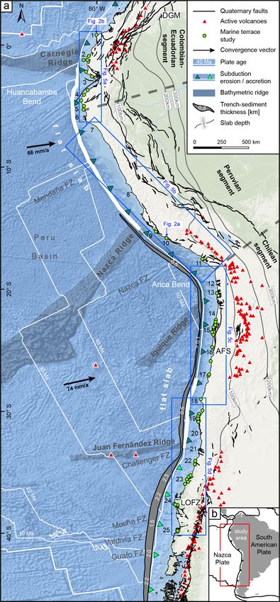
2488                                          R. Freisleben et al.: Marine terraces along the Pacific coast of South America

1   Introduction                                                  shoreline angle. The marine terrace morphology comprises
                                                                  a gently inclined erosional or depositional paleo-platform
Tectonically active coasts are highly dynamic geomorphic          that terminates landward at a steeply sloping paleo-cliff sur-
environments, and they host densely populated centers and         face. The intersection point between both surfaces represents
associated infrastructure (Melet et al., 2020). Coastal areas     the approximate sea-level position during the formation of
have been episodically affected by the effects of sea-level       the marine terrace, also known as shoreline angle; if coastal
changes at glacial timescales, modifying the landscape and        uplift is rapid, such uplifting abrasion or depositional sur-
leaving behind fossil geomorphic markers, such as former          faces may be preserved in the landscape and remain unal-
paleo-shorelines and marine terraces (Lajoie, 1986). One of       tered by the effects of subsequent sea-level oscillations (La-
the most prominent coastal landforms are marine terraces          joie, 1986).
that were generated during the protracted last interglacial          The analysis of elevation patterns based on shoreline-angle
sea-level highstand that occurred ∼ 125 kyr ago (Siddall et       measurements at subduction margins has been largely used
al., 2006; Hearty et al., 2007; Pedoja et al., 2011). These       to estimate vertical deformation rates and the mechanisms
terraces are characterized by a higher preservation potential     controlling deformation, including the interaction of the up-
which facilitates their recognition, mapping, and lateral cor-    per plate with bathymetric anomalies, the activity of crustal
relation. Furthermore, because of their high degree of preser-    faults in the upper plate, and deep-seated processes such as
vation and relatively young age, they have been used to esti-     basal accretion of subducted trench sediments (Taylor et al.,
mate vertical deformation rates at local and regional scales.     1987; Hsu, 1992; Macharé and Ortlieb, 1992; Ota et al.,
The relative abundance and geomorphic characteristics of the      1995; Pedoja et al., 2011; Saillard et al., 2011; Jara-Muñoz
last interglacial marine terraces make them ideal geomorphic      et al., 2015; Melnick, 2016). The shoreline angle represents a
markers with which to reconstruct past sea-level positions        1D descriptor of the marine terrace elevation whose measure-
and to enable comparisons between distant sites under dif-        ments are reproducible when using quantitative morphome-
ferent climatic and tectonic settings.                            tric approaches (Jara-Muñoz et al., 2016). Furthermore, the
   The western South American coast (WSAC) is a tecton-           estimation of the marine terrace elevations based on shore-
ically active region that has been repeatedly affected by         line angles can be further improved by quantifying their re-
megathrust earthquakes and associated surface deformation         lationship with paleo sea level, also known as the indicative
(Beck et al., 1998; Melnick et al., 2006; Bilek, 2010; Baker      meaning (Lorscheid and Rovere, 2019).
et al., 2013). Interestingly, previous studies have shown that       In this continental-scale compilation of marine terrace ele-
despite the broad spectrum of latitudinal climatic conditions     vations along the WSAC, we present systematically mapped
and erosional regimes along the WSAC, marine terraces are         shoreline angles of marine terraces of the last (Eemian–
scattered but omnipresent along the coast (Ota et al., 1995;      Sangamonian) interglacial obtained along 5000 km of coast-
Regard et al., 2010; Rehak et al., 2010; Bernhardt et al.,        line between 1◦ N and 40◦ S. In this synthesis we rely on
2016, 2017; Melnick, 2016). However, only a few studies on        chronological constraints from previous regional studies and
interglacial marine terraces have been conducted along the        compilations (Pedoja et al., 2011). For the first time we are
WSAC, primarily in specific areas where they are best ex-         able to introduce an almost continuous pattern of terrace el-
pressed; this has resulted in disparate and inconclusive ma-      evation and coastal uplift rates at a spatial scale of 103 km
rine terrace measurements based on different methodological       along the WSAC. Furthermore, in our database we com-
approaches and ambiguous interpretations concerning their         pare tectonic and climatic parameters to elucidate the mech-
origin in a tectonic and climatic context (Hsu et al., 1989;      anisms controlling the formation and preservation of marine
Ortlieb and Macharé, 1990; Hsu, 1992; Macharé and Ortlieb,        terraces and patterns of crustal deformation along the coast.
1992; Pedoja et al., 2006b, 2011; Saillard et al., 2009, 2011;    This study was thus primarily intended to provide a compre-
Rodríguez et al., 2013). This lack of reliable data points has    hensive, standardized database and description of last inter-
revealed a need to re-examine the last interglacial marine ter-   glacial marine terrace elevations along the tectonically ac-
races along the WSAC based on standardized methodologies          tive coast of South America. This database therefore war-
in order to obtain a systematic and continuous record of ma-      rants future research into coastal environments to decipher
rine terrace elevations along the coast. This information is      potential tectonic forcings with regard to the deformation
crucial in order to increase our knowledge of the climatic        and seismotectonic segmentation of the forearc; as such this
and tectonic forcing mechanisms that contributed to the for-      database will ultimately help to decipher the relationship be-
mation and degradation of marine terraces in this region.         tween upper-plate deformation, vertical motion, and bathy-
   Marine terrace sequences at tectonically active coasts are     metric anomalies and aid in the identification of regional
landforms formed by wave erosion and/or accumulation of           fault motions along pre-existing anisotropies in the South
sediments resulting from the interaction between tectonic         American continental plate. Finally, our database includes in-
uplift and superposed oscillating sea-level changes (Lajoie,      formation on climate-driving forcing mechanisms that may
1986; Anderson et al., 1999; Jara-Muñoz et al., 2015). Typ-       influence the formation, modification, and/or destruction of
ically, marine terrace elevations are estimated based on the      marine terraces in different climatic sectors along the South

Earth Syst. Sci. Data, 13, 2487–2513, 2021                                        https://doi.org/10.5194/essd-13-2487-2021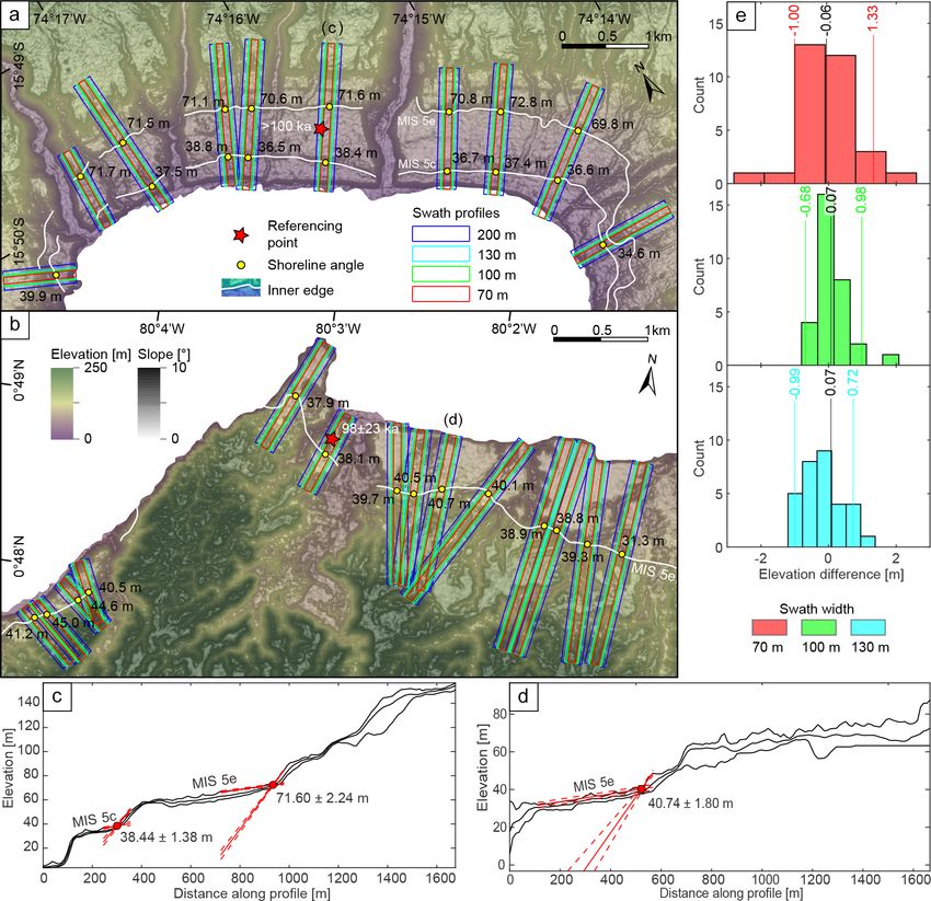
R. Freisleben et al.: Marine terraces along the Pacific coast of South America                                            2489

American convergent margin. This new database is part of         spect to the convergence direction resulted in 500 km SE-
the World Atlas of Last Interglacial Shorelines (WALIS),         directed migration of its locus of ridge subduction during
published online at https://doi.org/10.5281/zenodo.4309748       the last 10 Myr (Hampel, 2002; Saillard et al., 2011; Mar-
(Freisleben et al., 2020).                                       tinod et al., 2016a). Similarly, smaller aseismic ridges such
                                                                 as the Juan Fernández Ridge and the Iquique Ridge subduct
                                                                 beneath the South American continent at 32 and 21◦ S, re-
2     Geologic and geomorphic setting of the WSAC                spectively. The intercepts between these bathymetric anoma-
                                                                 lies and the upper plate are thought to influence the charac-
2.1     Tectonic and seismotectonic characteristics              teristics of interplate coupling and seismic rupture (Bilek et
2.1.1    Subduction geometry and bathymetric features            al., 2003; Wang and Bilek, 2011; Geersen et al., 2015; Col-
                                                                 lot et al., 2017) and mark the boundaries between flat and
The tectonic setting of the convergent margin of South Amer-     steep subduction segments and changes between subduction
ica is controlled by subduction of the oceanic Nazca plate       erosion and accretion (Jordan et al., 1983; von Huene et al.,
beneath the South American continental plate. The conver-        1997; Ramos and Folguera, 2009) (Fig. 1).
gence rate varies between 66 mm yr−1 in the north (8◦ S lat-        In addition to bathymetric anomalies, several studies have
itude) and 74 mm yr−1 in the south (27◦ S latitude) (Fig. 1).    shown that variations in the volume of sediments in the
The convergence azimuth changes slightly from 81.7◦ N to-        trench may control the subduction regime from an erosional
ward 77.5◦ N from north to south (DeMets et al., 2010). The      mode to an accretionary mode (von Huene and Scholl, 1991;
South American subduction zone is divided into four ma-          Bangs and Cande, 1997). In addition, the volume of sedi-
jor segments with variable subduction angles inferred from       ment in the trench has also been hypothesized to influence
the spatial distribution of Benioff seismicity (Barazangi and    the style of interplate seismicity (Lamb and Davis, 2003).
Isacks, 1976; Jordan et al., 1983) (Fig. 1). The segments be-    At the southern Chilean margin, thick trench-sediment se-
neath northern and central Peru (2–15◦ S) and beneath cen-       quences and a steeper subduction angle correlate primarily
tral Chile (27–33◦ S) are characterized by a gentle dip of the   with subduction accretion, although the area of the intercept
subducting plate between 5 and 10◦ at depths of ∼ 100 km         of the continental plate with the Chile Rise spreading cen-
(Hayes et al., 2018), whereas the segments beneath south-        ter locally exhibits the opposite case (von Huene and Scholl,
ern Peru and northern Chile (15–27◦ S) and beneath southern      1991; Bangs and Cande, 1997). Subduction erosion charac-
Chile (33–45◦ S) have steeper dips of 25–30◦ . Spatial dis-      terizes the region north of the southern volcanic zone from
tributions of earthquakes furthermore indicate a steep-slab      central and northern Chile to southern Peru (33–15◦ S) due to
subduction segment in Ecuador and southern Colombia (2◦ S        decreasing sediment supply to the trench, especially within
to 5◦ N) and a flat-slab segment in NW Colombia (north of        the flat-slab subduction segments (Stern, 1991; von Huene
5◦ N) (Pilger, 1981; Cahill and Isacks, 1992; Gutscher et al.,   and Scholl, 1991; Bangs and Cande, 1997; Clift and Van-
2000; Ramos and Folguera, 2009). Processes that have been        nucchi, 2004). Clift and Hartley (2007) and Lohrmann et
inferred to be responsible for the shallowing of the subduc-     al. (2003) argued for an alternate style of slow tectonic ero-
tion slab include the subduction of large buoyant ridges or      sion leading to underplating of subducted material below the
plateaus (Espurt et al., 2008), as well as the combination of    base of the crustal forearc, which is synchronous with tec-
the trenchward motion of thick, buoyant continental litho-       tonic erosion beneath the trenchward part of the forearc. For
sphere accompanied by trench retreat (Sobolev and Babeyko,       the northern Andes, several authors also classify the subduc-
2005; Manea et al., 2012). Volcanic activity, as well as the     tion zone as an erosional type (Clift and Vannucchi, 2004;
forearc architecture and distribution of upper-plate deforma-    Scholl and Huene, 2007; Marcaillou et al., 2016).
tion, further emphasizes the location of flat-slab subduction
segments (Jordan et al., 1983; Kay et al., 1987; Ramos and       2.1.2   Major continental fault systems in the coastal
Folguera, 2009).                                                         realm
   Several high bathymetric features have been recognized on
the subducting Nazca plate. The two most prominent bathy-        The South American convergent margin comprises several
metric features being subducted beneath South America are        fault systems with different kinematics whose presence is
the Carnegie and Nazca aseismic ridges at 0 and 15◦ S, re-       closely linked to oblique subduction and the motion and de-
spectively; they consist of seamounts related to hot-spot vol-   formation of forearc slivers. Here we summarize the main
canism (Gutscher et al., 1999; Hampel, 2002). The 300 km         structures that affect the Pacific coastal areas. North of the
wide and ∼ 2 km high Carnegie Ridge subducts roughly par-        Talara bend (5◦ S), active thrusting and dextral strike-slip
allel to the convergence direction, and its geometry should      faulting dominate the coastal lowlands of Ecuador (e.g.,
have remained relatively stable beneath the continental plate    Mache, Bahía, Jipijapa faults), although normal faulting also
(Angermann et al., 1999; Gutscher et al., 1999; DeMets et        occurs at Punta Galera (Cumilínche fault) and the Manta
al., 2010; Martinod et al., 2016a). In contrast, the obliquity   Peninsula (Río Salado fault) (Fig. 1). Farther south, normal
of the 200 km wide and 1.5 km high Nazca Ridge with re-          faulting is active in the Gulf of Guayaquil (Posorja fault),

https://doi.org/10.5194/essd-13-2487-2021                                       Earth Syst. Sci. Data, 13, 2487–2513, 2021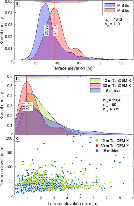
2490                                           R. Freisleben et al.: Marine terraces along the Pacific coast of South America

and dextral strike-slip faulting occurs at the Santa Elena         Gulf of Guayaquil (3◦ S) and the Dolores–Guayaquil megas-
Peninsula (La Cruz fault) (Veloza et al., 2012; Costa et al.,      hear separate the northern from the southern forearc units.
2020). The most prominent dextral fault in this region is          The coast-trench distance along the Huancabamba bend is
the 2000 km long, NE-striking Dolores–Guayaquil megas-             quite small (∼ 55–90 km), except for the Gulf of Guayaquil,
hear (DGM) which starts in the Gulf of Guayaquil and termi-        and the trench east of the Carnegie Ridge is at a relatively
nates in the Colombian hinterland east of the range-bounding       shallow depth of ∼ 3.5 km. Farther south, the Peruvian fore-
thrust faults of the Colombian Andes (Veloza et al., 2012;         arc comprises the up to 160 km wide Coastal Plains in the
Villegas-Lanza et al., 2016; Costa et al., 2020) (Fig. 1). Nor-    north and the narrow, 3000 m high Western Cordillera. While
mal faults have been described along the coast of Peru at the      the Coastal Plains in north-central Peru are relatively nar-
Illescas Peninsula in the north (6◦ S), within the El Huevo–       row (< 40 km), they widen in southern Peru, and the eleva-
Lomas fault system in the San Juan de Marcona area (14.5–          tion of the Western Cordillera increases to more than 5000 m
16◦ S), and within the Incapuquio fault system farther south       (Suárez et al., 1983; Jaillard et al., 2000). The region between
(17–18◦ S) (Veloza et al., 2012; Villegas-Lanza et al., 2016;      the coast and the trench in central Peru (up to 220 km) nar-
Costa et al., 2020). The main fault zones of the Chilean con-      rows toward the San Juan de Marcona area (∼ 75 km) near
vergent margin comprise the Atacama fault system (AFS) in          the intercept with the Nazca Ridge, and the relatively deep
the Coastal Cordillera extending from Iquique to La Serena         trench (∼ 6.5 km) becomes shallower (< 5 km) (GEBCO
(29.75◦ S; Fig. 1) with predominantly north–south-striking         Bathymetric Compilation Group, 2020). Between 18 and
normal faults, which result in the relative uplift of their        28◦ S, the Chilean forearc comprises the 50 km wide and
western side (e.g., Mejillones fault, Salar del Carmen fault)      up to 2700 m high Coastal Cordillera, which is separated
(Naranjo, 1987; González and Carrizo, 2003; Cembrano et            from the Precordillera by the Central Depression. In the flat-
al., 2007). Coastal fault systems farther south are located        slab subduction segment between 27 and 33◦ S there is nei-
in the Altos de Talinay area (30.5◦ S; Puerto Aldea fault),        ther a morphotectonic region characterized by a central de-
near Valparaíso (33◦ S; Quintay and Valparaíso faults), near       pression nor active volcanism in the high Andean cordillera
the Arauco Peninsula (36–39◦ S; Santa María and Lanalhue           (Fig. 1) (Jordan et al., 1983). The Chilean forearc comprises
faults), and in between these areas (Topocalma, Pichilemu,         the Coastal Cordillera, which varies in altitude from up to
Carranza, and Pelluhue faults) (Ota et al., 1995; Melnick et       2000 m at 33◦ S to 500 m at 46◦ S, and the Central Depression
al., 2009, 2020; Santibáñez et al., 2019; Maldonado et al.,        that separates the forearc from the Main Cordillera. From the
2021) (Fig. 1). However, there is still limited knowledge re-      Arica bend, where the coast-trench distance is up to 170 km
garding Quaternary slip rates and kinematics and, most im-         and the trench ∼ 8 km deep, a slight increase in coast-trench
portantly, the location of active faults along the forearc re-     distance can be observed in Chile toward the south (∼ 80–
gion of South America (Jara-Muñoz et al., 2018; Melnick et         130 km), as can a decrease in trench depth to ∼ 4.5 km.
al., 2019).
                                                                   2.2.2   Marine terraces and coastal uplift rates
2.2     Climate and geomorphic setting                             Wave erosion generates wave-cut terrace levels, while the
2.2.1    Geomorphology                                             accumulation of shallow marine sediments during sea-level
                                                                   highstands forms wave-built terraces. Another type of ter-
The 8000 km long Andean orogen is a major, hemisphere-             race is known as “rasa” and refers to wide shore platforms
scale feature that can be divided into segments with dis-          formed under slow-uplift conditions (< 0.2 m kyr−1 ) and the
tinctive geomorphic and tectonic characteristics. The princi-      repeated reoccupation of this surface by high sea levels (Re-
pal segments comprise the NNE–SSW-trending Colombian–              gard et al., 2010; Rodríguez et al., 2013; Melnick, 2016).
Ecuadorian segment (12◦ N–5◦ S), the NW–SE-oriented Pe-            Other studies indicate a stronger influence of climate and
ruvian segment (5–18◦ S), and the north–south-trending             rock resistance to erosion compared to marine wave action
Chilean segment (18–56◦ S) (Jaillard et al., 2000) (Fig. 1).       (Prémaillon et al., 2018). Typically, the formation of Pleis-
Two major breaks separate these segments; these are the            tocene marine terraces in the study area occurred during in-
Huancabamba bend in northern Peru and the Arica bend at            terglacial and interstadial relative sea-level highstands that
the Peru–Chile border. The distance of the trench from the         were superposed on the uplifting coastal areas; according to
WSAC coastline averages 118 km and ranges between 44 and           the Quaternary oxygen-isotope curve defining warm and cold
217 km. The depth of the trench varies between 2920 and            periods, high Quaternary sea levels have been correlated with
8177 m (GEBCO Bathymetric Compilation Group, 2020),                warm periods and are denoted with the odd-numbered Ma-
and the continental shelf has an average width of 28 km (Paris     rine Isotope Stages (MISs) (Lajoie, 1986; Shackleton et al.,
et al., 2016).                                                     2003).
   In the 50 to 180 km wide coastal area of the Ecuadorian            Along the WSAC, staircase-like sequences of multiple
Andes, where the Western Cordillera is flanked by a struc-         marine terraces are preserved nearly continuously along the
tural depression, relief is relatively low (< 300 m a.s.l.). The   coast. These terraces comprise primarily wave-cut surfaces

Earth Syst. Sci. Data, 13, 2487–2513, 2021                                         https://doi.org/10.5194/essd-13-2487-2021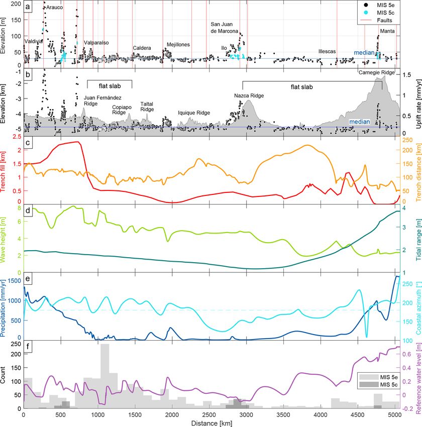
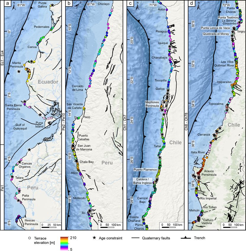
R. Freisleben et al.: Marine terraces along the Pacific coast of South America                                                           2491

Figure 1. (a) Morphotectonic setting of the South American margin showing major fault systems and crustal faults (Costa et al., 2000;
Veloza et al., 2012; Maldonado et al., 2021), slab depth (Hayes et al., 2018), flat-slab subduction segments, active volcanos (Venzke, 2013),
bathymetric features of the subducting plate, trench-sediment thickness (Bangs and Cande, 1997), segments of subduction erosion and
accretion (Clift and Vannucchi, 2004), plate age (Müller et al., 2008), convergence vectors (DeMets et al., 2010), and marine terrace ages
used for lateral correlation. DGM: Dolores–Guayaquil megashear; AFS: Atacama fault system; LOFZ: Liquiñe–Ofqui fault zone; FZ: fracture
zone; 1: Punta Galera; 2: Manta Pen.; 3: Gulf of Guayaquil, Santa Elena Pen.; 4: Tablazo Lobitos; 5: Paita Pen.; 6: Illescas Pen.; 7: Chiclayo;
8: Lima; 9: San Juan de Marcona; 10: Chala Bay; 11: Pampa del Palo; 12: Pisagua; 13: Iquique; 14: Tocopilla; 15: Mejillones Pen.; 16:
Taltal; 17: Caldera; 18: Punta Choros; 19: Altos de Talinay; 20: Los Vilos; 21: Valparaíso; 22: Topocalma; 23: Carranza; 24: Arauco Pen.;
25: Valdivia (World Ocean Basemap: Esri, Garmin, GEBCO, NOAA NGDC, and other contributors). (b) Location of the study area.

https://doi.org/10.5194/essd-13-2487-2021                                                  Earth Syst. Sci. Data, 13, 2487–2513, 2021
2492                                            R. Freisleben et al.: Marine terraces along the Pacific coast of South America

that are frequently covered by beach ridges of siliciclastic        ranza (110 m) and to very low elevations in between (15 m)
sediments and local accumulations of carbonate bioclastic           (Melnick et al., 2009; Jara-Muñoz et al., 2015).
materials (Ota et al., 1995; Saillard et al., 2009; Rodríguez et       Coastal uplift-rate estimates along the WSAC mainly
al., 2013; Martinod et al., 2016b). Rasa surfaces exist in the      comprise calculations for the Talara Arc, the San Juan de
regions of southern Peru and northern Chile (Regard et al.,         Marcona area, the Mejillones Peninsula, the Altos de Tali-
2010; Rodríguez et al., 2013; Melnick, 2016). Particularly          nay area, and several regions in south-central Chile. Along
the well-preserved MIS 5e terrace level has been largely used       the Talara Arc (6.5◦ S–1◦ N), marine terraces of the Manta
as a strain marker in the correlation of uplifted coastal sec-      Peninsula and La Plata Island in central Ecuador indicate
tors due to its lateral continuity and high potential for preser-   the most pronounced uplift rates of 0.31–0.42 m kyr−1 since
vation. Global observations of sea-level fluctuations during        MIS 5e, while similar uplift rates are documented to the
MIS 5 allow us to differentiate between three second-order          north in the Esmeraldas area (0.34 m kyr−1 ) and lower ones
highstands at 80 ka (5a), 105 ka (5c), and 128 to 116 ka (5e)       to the south at the Santa Elena Peninsula (0.1 m kyr−1 ). In
with paleo sea levels of −20 m for both of the younger and          northern Peru, last interglacial uplift rates are relative low,
+3 ± 3 m for the oldest highstand (Stirling et al., 1998; Sid-      ranging from 0.17–0.21 m kyr−1 for the Tablazo Lobitos and
dall et al., 2006; Hearty et al., 2007; Rohling et al., 2009;       0.16 m kyr−1 for the Paita Peninsula to 0.12 m kyr−1 for the
Pedoja et al., 2011), although glacio-isostatic adjustments         Bay of Bayovar and the Illescas Peninsula (Pedoja et al.,
(GIAs) can cause local differences of up to 30 m (Simms et          2006b, a). Marine terraces on the continental plate above the
al., 2016; Creveling et al., 2017). The database generated in       subducting Nazca Ridge (13.5–15.6◦ S) record variations in
this study is based exclusively on the last interglacial ma-        uplift rate where the coastal forearc above the northern flank
rine terraces exposed along the WSAC between Ecuador and            of the ridge is either stable or has undergone net subsidence
southern Chile (1–40◦ S). In the following section we present       (Macharé and Ortlieb, 1992). The coast above the ridge crest
a brief review of previously studied marine terrace sites in        has been rising at about 0.3 m kyr−1 and the coast above the
this area.                                                          southern flank (San Juan de Marcona) has been uplifting at
   Paleo-shoreline elevations of the last interglacial (MIS 5e)     a rate of 0.5 m kyr−1 (Hsu, 1992) or even 0.7 m kyr−1 (Or-
in Ecuador are found at elevations of around 45 ± 2 m a.s.l. in     tlieb and Macharé, 1990) for at least the last 125 kyr. Saillard
Punta Galera (Esmeraldas area), 43–57 ± 2 m on the Manta            et al. (2011) state that long-term regional uplift in the San
Peninsula and La Plata Island, and 15 ± 5 m a.s.l. on the           Juan de Marcona area has increased since about 800 ka re-
Santa Elena Peninsula (Pedoja et al., 2006b, a). In north-          lated to the southward migration of the Nazca Ridge, and
ern Peru, MIS 5e terraces have been described at elevations         it ranges from 0.44 to 0.87 m kyr−1 . The Pampa del Palo
of 18–31 m a.s.l. for the Tablazo Lobitos (Cancas and Man-          area in southern Peru rose more slowly or was even down-
cora areas), at 25 ± 5 m a.s.l. on the Paita Peninsula, and at      faulted and had subsided with respect to the adjacent coastal
18 ± 3 m a.s.l. on the Illescas Peninsula and the Bay of Bay-       regions (Ortlieb et al., 1996b). These movements ceased af-
ovar (Pedoja et al., 2006b). Farther south, MIS 5e terraces are     ter the highstand during the MIS 5e, and slow-uplift rates
exceptionally high in the San Juan de Marcona area imme-            of approximately 0.16 m kyr−1 have characterized the region
diately south of the subducting Nazca Ridge, with maximum           since 100 ka (Ortlieb et al., 1996b). In northern Chile (24–
elevations of 80 m at the Cerro Trés Hermanas and 105 m at          32◦ S), uplift rates for the Late Pleistocene average around
the Cerro El Huevo (Hsu et al., 1989; Ortlieb and Macharé,          0.28 ± 0.15 m kyr−1 (Martinod et al., 2016b), except for the
1990; Saillard et al., 2011). The Pampa del Palo region in          Altos de Talinay area where pulses of rapid uplift occurred
southern Peru exhibits relatively thick vertical stacks of shal-    during the Middle Pleistocene (Ota et al., 1995; Saillard et
low marine terrace deposits related to MIS 7, 5e (∼ 20 m),          al., 2009; Martinod et al., 2016b). The Central Andean rasa
and 5c that may indicate a different geodynamic behavior            (15–33◦ S) and Lower to Middle Pleistocene shore platforms
compared to adjacent regions (Ortlieb et al., 1996b). In cen-       – which are also generally wider – indicate a period of tec-
tral and northern Chile, the terrace levels of the last inter-      tonic stability or subsidence followed by accelerated and spa-
glacial occur at 250–400, 150–240, 80–130, and 30–40 m              tially continuous uplift after ∼ 400 ka (MIS 11) (Regard et
and in southern Chile at 170–200, 70, 20–38, and 8–10 m             al., 2010; Rodríguez et al., 2013; Martinod et al., 2016b).
(Fuenzalida et al., 1965). Specifically, between 24 and 32◦ S,      However, according to Melnick (2016), the central Andean
paleo-shoreline elevations of the last interglacial (MIS 5e)        rasa has experienced slow and steady long-term uplift with a
range between 25 and 45 m (Ota et al., 1995; Saillard et al.,       rate of 0.13 ± 0.04 m kyr−1 during the Quaternary, predom-
2009; Martinod et al., 2016b). Shore platforms are higher in        inantly accumulating strain through deep earthquakes at the
the Altos de Talinay area (30.3–31.3◦ S) but are small, poorly      crust–mantle boundary (Moho) below the locked portion of
preserved, and terminate at a high coastal scarp between            the plate interface. The lowest uplift rates occur at the Arica
26.75 and 24◦ S (Martinod et al., 2016b). Shoreline-angle           bend and increase gradually southward; the highest values
elevations between 34 and 38◦ S (along the Maule seismo-            are attained along geomorphically distinct peninsulas (Mel-
tectonic segment) vary from high altitudes in the Arauco and        nick, 2016). In the Maule segment (34–38◦ S), the mean up-
Topocalma areas (200 m) to moderate elevations near Car-            lift rate for the MIS 5 terrace level is 0.5 m kyr−1 , exceeded

Earth Syst. Sci. Data, 13, 2487–2513, 2021                                          https://doi.org/10.5194/essd-13-2487-2021

R. Freisleben et al.: Marine terraces along the Pacific coast of South America 2493
only in the areas of Topocalma, Carranza, and Arauco, where 3.1 Mapping of marine terraces
it amounts to 1.6 m kyr−1 (Melnick et al., 2009; Jara-Muñoz
et al., 2015). Although there are several studies of marine ter- Marine terraces are primarily described based on their ele-
races along the WSAC, these are isolated and based on dif- vation, which is essential for determining vertical deforma-
ferent methodological approaches, mapping and leveling res- tion rates. The measurements of the marine terrace eleva-
olutions, and dating techniques, which make regional com- tions of the last interglacial were performed using TanDEM-
parisons and correlations difficult in the context of the data X topography (12 and 30 m horizontal resolution) (German
presented here. Aerospace Center, DLR, 2018) and digital terrain models
from lidar (1, 2.5, and 5 m horizontal resolution). The dig-
2.2.3 Climate ital elevation models (DEMs) were converted to orthometric
heights by subtracting the EGM2008 geoid and projected in
Apart from latitudinal temperature changes, the present-day the universal transverse mercator (UTM) coordinate system
morphotectonic provinces along the South American mar- using the World Geodetic System (WGS1984) using zone
gin have a pronounced impact on the precipitation gradi- 19S for Chile, zone 18S for southern and central Peru, and
ents on the west coast of South America. Since mountain zone 17S for northern Peru and Ecuador.
ranges are oriented approximately perpendicular to moisture- To trace the MIS 5 shoreline, we mapped its inner edge
bearing winds, they affect both flanks of the orogen (Strecker along the west coast of South America based on slope
et al., 2007). The regional-scale pattern of wind circulation changes in TanDEM-X topography at the foot of paleo-cliffs
is dominated by westerly winds at subtropical and extratrop- (Jara-Muñoz et al., 2016) (Fig. 2a and b). To facilitate map-
ical latitudes primarily up to about 27◦ S (Garreaud, 2009). ping, we used slope and hillshade maps. We correlated the re-
However, anticyclones over the South Pacific result in winds sults of the inner-edge mapping with the marine terraces cata-
blowing from the south along the coast between 35◦ S and log of Pedoja et al. (2011) and references therein (Sect. 2.2.2,
10◦ S (Garreaud, 2009). The moisture in the equatorial An- Table 1). Further references used to validate MIS 5e ter-
des (Ecuador and Colombia) and in the areas farther south race heights include Victor et al. (2011) for the Pampa de
(27◦ S) is fed by winds from the Amazon basin and the Mejillones, Martinod et al. (2016b) for northern Chile, and
Gulf of Panama, resulting in rainfall mainly on the eastern Jara-Muñoz et al. (2015) for the area between 34 and 38◦ S.
flanks of the mountain range (Bendix et al., 2006; Bookhagen We define the term “referencing point” for these previously
and Strecker, 2008; Garreaud, 2009). The Andes of southern published terrace heights and age constraints. The referenc-
Ecuador, Peru, and northern Chile are dominated by a rain- ing point with the shortest distance to the location of our
shadow effect that causes aridity within the Andean Plateau measurements served as a topographical and chronological
(Altiplano-Puna), the Western Cordillera, and the coastal re- benchmark for mapping the MIS 5 terrace in the respective
gion (Houston and Hartley, 2003; Strecker et al., 2007; Gar- areas. In addition, this distance is used to assign a quality
reaud, 2009). Furthermore, the aridity is exacerbated by the rating (QR) to our measurements.
effects of the cold Humboldt current which prevents hu- In addition to MIS 5e, we also mapped MIS 5c in areas
midity from the Pacific from penetrating inland (Houston with high uplift rates such as at the Manta Peninsula, San
and Hartley, 2003; Garreaud, 2009; Coudurier-Curveur et Juan de Marcona, Topocalma, Carranza, and Arauco. Al-
al., 2015). The precipitation gradient reverses between 27 though we observed a terrace level correlated to MIS 5a in
and 35◦ S where the Southern Hemisphere westerlies cause the Marcona area, we excluded this level from the database
abundant rainfall on the western flanks of the Coastal and due to its limited preservation at other locations and lack of
Main cordilleras (Garreaud, 2009). Martinod et al. (2016b) chronological constraints. Our assignment of mapped terrace
proposed that latitudinal differences in climate largely influ- levels to MIS 5c is primarily based on age constraints by Sail-
ence coastal morphology, specifically the formation of high lard et al. (2011) for the Marcona area and Jara-Muñoz et
coastal scarps that prevent the development of extensive ma- al. (2015) for the area between 34 and 38◦ S. However, in or-
rine terrace sequences. However, the details of this relation- der to evaluate the possibility that our correlation with MIS
ship have not been conclusively studied along the full extent 5c is flawed, we estimated uplift rates for the lower terraces
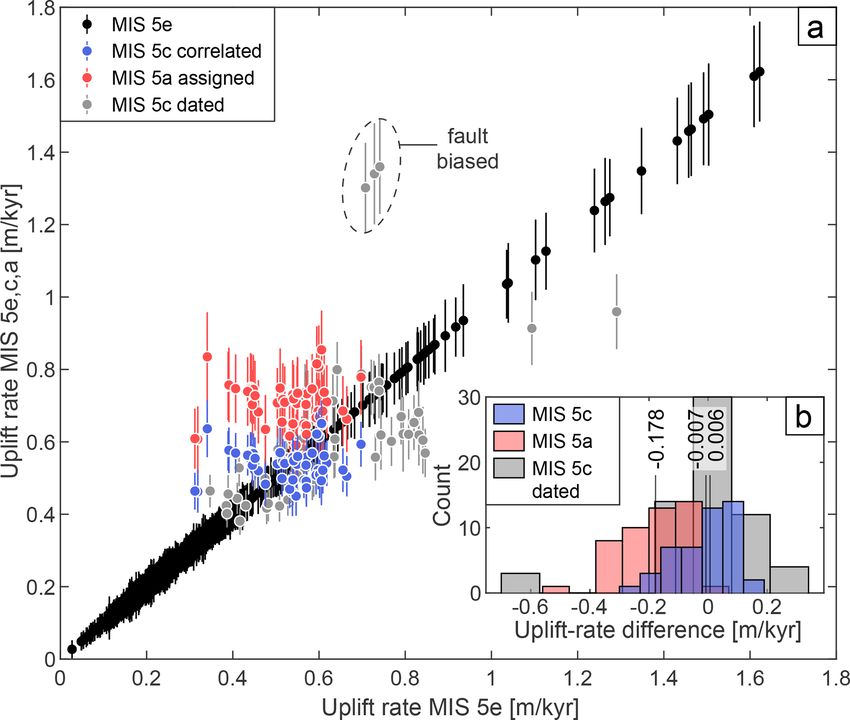
of the Pacific coast of South America. by assigning them tentatively to either MIS 5a or MIS 5c. We
interpolated the uplift rates derived from the MIS 5e level at
3 Methods the sites of the lower terraces and compared the differences
(Fig. 3a). If we infer that uplift rates were constant in time at
We combined – and describe in detail below – bibliographic each site throughout the three MIS 5 substages, the compari-
information, different topographic data sets, and uniform son suggests these lower terrace levels correspond to MIS 5c
morphometric and statistical approaches to assess the eleva- because of the smaller difference in uplift rate rather than to
tion of marine terraces and accompanying vertical deforma- MIS 5a (Fig. 3b).
tion rates along the western South American margin. A rigorous assessment of marine terrace elevations is
crucial for determining accurate vertical deformation rates.
https://doi.org/10.5194/essd-13-2487-2021 Earth Syst. Sci. Data, 13, 2487–2513, 20212494 R. Freisleben et al.: Marine terraces along the Pacific coast of South America Figure 2. Orthometrically corrected TanDEM-X and slope map of (a) Chala Bay in south-central Peru and (b) Punta Galera in northern Ecuador with mapped inner shoreline edges of the MIS 5e and 5c terrace levels. Colored rectangles represent swath-profile boxes of various widths that were placed perpendicular to the inner edges for the subsequent estimation of terrace elevation in TerraceM. The red star indicates the referencing point with the age constraint for the respective area (Pedoja et al., 2006b; Saillard, 2008). Panels (c) and (d) show the estimation of shoreline-angle elevations in TerraceM by intersecting linear-regression fits of the paleo-cliff and paleo-platform (200 m wide swath profiles). (e) Histograms of elevation differences measured in both areas for various swath widths (70, 100, and 130 m) with respect to the 200 m wide reference swath profile (blue). Vertical lines indicate median values and standard deviations (2σ ). Since fluvial degradation and hillslope processes subsequent terrace elevations and vertical deformation rates (Jara-Muñoz to the abandonment of marine terraces may alter terrace mor- et al., 2015). To precisely measure the shoreline-angle eleva- phology (Anderson et al., 1999; Jara-Muñoz et al., 2015), tions of the MIS 5 terrace level, we used a profile-based ap- direct measurements of terrace elevations at the inner edge proach in TerraceM, a graphical user interface in MATLAB® (foot of the paleo-cliff) may result in overestimation of the (Jara-Muñoz et al., 2016); http://www.terracem.com/ (last Earth Syst. Sci. Data, 13, 2487–2513, 2021 https://doi.org/10.5194/essd-13-2487-2021
R. Freisleben et al.: Marine terraces along the Pacific coast of South America                                                              2495

Table 1. Age constraints used for mapping of the inner edge of MIS 5 and for verifying our terrace-elevation measurements. This compilation
is mainly based on the terrace catalog of Pedoja et al. (2011); added references include Victor et al. (2011) for Pampa de Mejillones, Martinod
et al. (2016b) for northern Chile, and Jara-Muñoz et al. (2015) for south-central Chile. Absolute ages refer to MIS 5e marine terraces unless
otherwise specified; inferred ages refer to their associated MIS. IRSL: infrared-stimulated luminescence, AAR: amino-acid racemization,
CRN: cosmogenic radionuclides, ESR: electron spin resonance.

   Country       Location                   Lat.    Long.   Dating method        Confidence    Reference                             Age (ka)
   Ecuador       Galera                    0.81    −80.03   IRSL                         5     Pedoja et al. (2006b)                  98 ± 23
   Ecuador       Manta                    −0.93    −80.66   IRSL, U/Th                   5     Pedoja et al. (2006b)           76 ± 18, 85 ± 1
   Ecuador       La Plata                 −1.26    −81.07   U/Th                         5     Pedoja et al. (2006b)                  104 ± 2
   Ecuador       Manta                    −1.27    −80.78   IRSL                         5     Pedoja et al. (2006b)                 115 ± 23
   Ecuador       Santa Elena              −2.21    −80.88   U/Th                         5     Pedoja et al. (2006b)          136 ± 4, 112 ± 2
   Ecuador       Puna                     −2.60    −80.40   U/Th                         5     Pedoja et al. (2006b)            98 ± 3, 95 ± 0
   Peru          Cancas                   −3.72    −80.75   Morphostratigraphy           5     Pedoja et al. (2006b)                    ∼ 125
   Peru          Mancora/Lobitos          −4.10    −81.05   Morphostratigraphy           5     Pedoja et al. (2006b)                    ∼ 125
   Peru          Talara                   −4.56    −81.28   Morphostratigraphy           5     Pedoja et al. (2006b)                    ∼ 125
   Peru          Paita                    −5.03    −81.06   Morphostratigraphy           5     Pedoja et al. (2006b)                    ∼ 125
   Peru          Bayovar/Illescas         −5.31    −81.10   IRSL                         5     Pedoja et al. (2006b)                  111 ± 6
   Peru          Cerro Huevo             −15.31    −75.17   CRN                          5     Saillard et al. (2011)           228 ± 28 (7e)
   Peru          Chala Bay               −15.85    −74.31   CRN                          5     Saillard (2008)                          > 100
   Peru          Ilo                     −17.55    −71.37   AAR                          5     Ortlieb et al. (1996b);                 ∼ 125,
                                                                                               Hsu et al. (1989)                       ∼ 105
   Chile         Punta Lobos             −20.35    −70.18   U/Th, ESR                    5     Radtke (1989)                            ∼ 125
   Chile         Cobija                  −22.55    −70.26   Morphostratigraphy           4     Ortlieb et al. (1995)             ∼ 125, ∼ 105
   Chile         Michilla                −22.71    −70.28   AAR                          3     Leonard and Wehmiller (1991)             ∼ 125
   Chile         Hornitos                −22.85    −70.30   U/Th                         5     Ortlieb et al. (1996a)         108 ± 1, 118 ± 6
   Chile         Chacaya                 −22.95    −70.30   AAR                          5     Ortlieb et al. (1996a)                   ∼ 125
   Chile         Pampa Mejillones        −23.14    −70.45   U/Th                         5     Victor et al. (2011)                   124 ± 3
   Chile         Mejillones/             −23.54    −70.55   U/Th, ESR                    3     Radtke (1989)                            ∼ 125
                 Punta Jorge
   Chile         Coloso                  −23.76    −70.46   ESR                          3     Schellmann and Radtke (1997)           106 ± 3
   Chile         Punta Piedras           −24.76    −70.55   CRN                          5     Martinod et al. (2016b)               138 ± 15
   Chile         Esmeralda               −25.91    −70.67   CRN                          5     Martinod et al. (2016b)                 79 ± 9
   Chile         Caldera                 −27.01    −70.81   U/Th, ESR                    5     Marquardt et al. (2004)                  ∼ 125
   Chile         Bahía Inglesa           −27.10    −70.85   U/Th, ESR                    5     Marquardt et al. (2004)                  ∼ 125
   Chile         Caleta Chañaral         −29.03    −71.49   CRN                          5     Martinod et al. (2016b)                138 ± 0
   Chile         Coquimbo                −29.96    −71.34   AAR                          5     Leonard and Wehmiller                    ∼ 125
                                                                                               (1992); Hsu et al. (1989)
   Chile         Punta Lengua de Vaca    −30.24    −71.63   U/Th                         5     Saillard et al. (2012)              95 ± 2 (5c)
   Chile         Punta Lengua de Vaca    −30.30    −71.61   U/Th                         5     Saillard et al. (2012)          386 ± 124 (11)
   Chile         Quebrada Palo Cortado   −30.44    −71.69   CRN                          5     Saillard et al. (2009)                149 ± 10
   Chile         Limarí River            −30.63    −71.71   CRN                          5     Saillard et al. (2009)           318 ± 30 (9c)
   Chile         Quebrada de la Mula     −30.79    −71.70   CRN                          5     Saillard et al. (2009)           225 ± 17 (7e)
   Chile         Quebrada del Teniente   −30.89    −71.68   CRN                          5     Saillard et al. (2009)           678 ± 51 (17)
   Chile         Puertecillo             −34.09    −71.94   IRSL                         5     Jara-Munoz et al. (2015)            87 ± 7 (5c)
   Chile         Pichilemu               −34.38    −71.97   IRSL                         5     Jara-Munoz et al. (2015)           106 ± 9 (5c)

https://doi.org/10.5194/essd-13-2487-2021                                                     Earth Syst. Sci. Data, 13, 2487–2513, 2021
2496 R. Freisleben et al.: Marine terraces along the Pacific coast of South America
Table 1. Continued.
Country Location Lat. Long. Dating method Confidence Reference Age (ka)
Chile Putu −35.16 −72.25 IRSL 5 Jara-Munoz et al. (2015) 85 ± 8 (5c)
Chile Constitucion −35.40 −72.49 IRSL 5 Jara-Munoz et al. (2015) 105 ± 8 (5c)
Chile Constitucion −35.44 −72.47 IRSL 5 Jara-Munoz et al. (2015) 124 ± 11
Chile Carranza −35.58 −72.61 IRSL 5 Jara-Munoz et al. (2015) 67 ± 6 (5c)
Chile Carranza −35.64 −72.54 IRSL 5 Jara-Munoz et al. (2015) 104 ± 9
Chile Pelluhue −35.80 −72.54 IRSL 5 Jara-Munoz et al. (2015) 112 ± 10
Chile Pelluhue −35.80 −72.55 IRSL 5 Jara-Munoz et al. (2015) 102 ± 9 (5c)
Chile Curanipe −35.97 −72.78 IRSL 5 Jara-Munoz et al. (2015) 265 ± 29
Chile Arauco −37.62 −73.67 IRSL 5 Jara-Munoz et al. (2015) 89 ± 9 (5c)
Chile Arauco −37.68 −73.57 CRN 5 Melnick et al. (2009) 127 ± 13
Chile Arauco −37.71 −73.39 CRN 5 Melnick et al. (2009) 133 ± 14
Chile Arauco −37.76 −73.38 CRN 5 Melnick et al. (2009) 130 ± 13
Chile Cerro Caleta Curiñanco −39.72 −73.40 Tephrochronology 4 Pino et al. (2002) ∼ 125
Chile South Curiñanco −39.76 −73.39 Tephrochronology 4 Pino et al. (2002) ∼ 125
Chile Valdivia −39.80 −73.39 Tephrochronology 4 Pino et al. (2002) ∼ 125
Chile Camping Bellavista −39.85 −73.40 Tephrochronology 4 Pino et al. (2002) ∼ 125
Chile Mancera −39.89 −73.39 Tephrochronology 5 Silva (2005) ∼ 125
Table 2. Median values and standard deviations (2σ ) representing the indicative meaning along the WSAC. The four sectors were chosen
based on their main geomorphic characteristics (see Sect. 4).
Upper limit of Lower limit of Reference Indicative
modern analog (m) modern analog (m) water level (m) range (m)
Ecuador and northern Peru 2.89 ± 0.16 −1.78 ± 0.47 0.54 ± 0.21 4.66 ± 0.65
Central and southern Peru 2.98 ± 0.31 −3.05 ± 0.52 −0.03 ± 0.11 6.06 ± 0.90
Northern Chile 3.01 ± 0.15 −2.89 ± 0.30 0.06 ± 0.08 5.90 ± 0.51
Central Chile 3.21 ± 0.19 −3.03 ± 0.38 0.07 ± 0.11 6.25 ± 0.60
access: 6 May 2021). We placed swath profiles of variable sections of these profiles, which represent the undisturbed
width perpendicular to the previously mapped inner edge, paleo-platform and paleo-cliff areas, were picked manually
which were used by the TerraceM algorithm to extract max- and fitted by linear regression. The extrapolated intersection
imum elevations to avoid areas of fluvial incision (Fig. 2a between both regression lines ultimately allowed us to de-
and b). For the placement of the swath profiles we tried termine the buried shoreline-angle elevation and associated
to capture a local representation of marine terrace topog- uncertainty, which is derived from the 95 % confidence in-
raphy with a sufficiently long, planar paleo-platform and a terval (2σ ) of both regressions (Fig. 2c and d). In total, we
sufficiently high paleo-cliff, simultaneously avoiding topo- measured 1843 MIS 5e and 110 MIS 5c shoreline-angle el-
graphic disturbance, such as colluvial wedges or areas af- evations. To quantify the paleo-position of the relative sea-
fected by incision. North of Caleta Chañaral (29◦ S), we used level elevation and the involved uncertainty for the WALIS
swath profiles of 200 m width, although we occasionally used database, we calculated the indicative meaning for each ma-
100 m wide profiles for narrow terrace remnants. South of rine terrace measurement using the IMCalc software from
29◦ S, we used swath widths of 130 and 70 m. The width Lorscheid and Rovere (2019). The indicative meaning com-
was chosen based on fluvial drainage densities that are as- prises the range between the lower and upper limits of sea-
sociated with precipitation gradients. Sensitivity tests com- level formation – the indicative range – as well as its mathe-
paring shoreline-angle measurements from different swath matically averaged position, which corresponds to the refer-
widths in the Chala Bay and at Punta Galera show only min- ence water level (Lorscheid and Rovere, 2019). Table 2 doc-
imal vertical deviations of less than 0.5 m (Fig. 2e). The
Earth Syst. Sci. Data, 13, 2487–2513, 2021 https://doi.org/10.5194/essd-13-2487-2021R. Freisleben et al.: Marine terraces along the Pacific coast of South America 2497
Figure 3. Comparison of MIS 5 uplift-rate estimates. (a) Uplift
rates derived by correlating mapped terrace occurrences located im-
mediately below the MIS 5e level to either MIS 5c (blue) or MIS 5a
(red) with respect to MIS 5e uplift rates. Marine terraces correlated
to MIS 5c by an age constraint are plotted in gray color. (b) His-
tograms of differences between MIS 5a or MIS 5c uplift rates and
MIS 5e uplift rates. Vertical lines show median uplift-rate differ-
ences. See Sect. 2.2.2 for relative sea-level elevations of MIS 5a,
5c, and 5e.
uments the medians and standard deviations of these values
for four extensive regions along the WSAC.
To quantify the reliability and consistency of our
shoreline-angle measurements, we developed a quality rating
from low (1) to high (5) confidence. Equation (1) illustrates
how we calculated the individual parameters and the overall
quality rating:
e
CRP DRP
QR = 1 + 2.4 × × 1− Figure 4. Influence of the parameters on the quality rating. The
max(CRP ) max (DRP ) x axis is the distance to reference point (RP), the y axis is the qual-
ity rating, and the color lines represent different values of quality-
ET
+ 1.2 × 1 − rating parameters. While one parameter is being tested, the remain-
max (ET )
ing parameters are set to their best values. That is why the QR does
R not reach values of 1 in the graphs displayed here. (a) Shoreline-
+ 0.4 × 1.2 × 1 − . (1)
max(R) angle elevation error. (b) Confidence value of the referencing point.
(c) Topographic resolution of the DEM used for terrace-elevation
The four parameters included in our quality rating (QR) com- estimation. (d) Histogram displaying the distribution of distances
prise (a) the distance to the nearest referencing point (DRP ), between each shoreline-angle measurement and its nearest RP (n:
(b) the confidence of the referencing point based on the dat- number of measurements). The red line is an exponential fit.
ing method used by previous studies (CRP ) (Pedoja et al.,
2011), (c) the measurement error in TerraceM (ET ), and
(d) the pixel-scale resolution of the topographic data set (R) qualification of Pedoja et al. (2011). The confidence depends
(Fig. 4). We did not include the error that results from the us- mainly on the reliability of the dating method but can be in-
age of different swath widths since the calculated elevation creased by good age constraints of adjacent terrace levels or
difference with respect to the most frequently used 200 m detailed morphostratigraphic correlations, such as in Chala
swath width is very low (< 0.5 m) (Fig. 2e). From the refer- Bay (Fig. 2a) (Goy et al., 1992; Saillard, 2008). We further
ence points we only used data points with a confidence value used this confidence value to quantify the quality of the age
of 3 or greater (1 – poor, 5 – very good) based on the previous constraints in the WALIS template.
https://doi.org/10.5194/essd-13-2487-2021 Earth Syst. Sci. Data, 13, 2487–2513, 20212498 R. Freisleben et al.: Marine terraces along the Pacific coast of South America
To account for the different uncertainties of the individual Vertical displacement rates and relative sea level are in-
parameters in the QR, we combined and weighted the param- fluenced by flexural rebound associated with loading and
eters DRP and CRP in a first equation claiming 60 % of the unloading of ice sheets during glacio-isostatic adjustments
final QR, ET in a second, and R in a third equation weighted (GIAs) (Stewart et al., 2000; Shepherd and Wingham, 2007).
30 % and 10 %, respectively. We justify these percentages by The amplitude and wavelength of GIAs is mostly determined
the fact that the distance and confidence to the nearest refer- by the flexural rigidity of the lithosphere (Turcotte and Schu-
encing point is of utmost importance for identifying the MIS bert, 1982) and should therefore not severely influence verti-
5e terrace level. The measurement error represents how well cal deformation along non-glaciated coastal regions (Rabassa
the mapping of the paleo-platform and paleo-cliff resulted in and Clapperton, 1990) that are located in the forearc of ac-
the shoreline-angle measurement, while the topographic res- tive subduction zones. This is supported by Creveling et
olution of the underlying DEM only influences the precise al. (2017) who showed no significant GIA along the WSAC
representation of the actual topography and has little impact between 1◦ N and 40◦ S since MIS 5a. Current GIA models
on the measurement itself. The coefficient assigned to the to- use an oversimplified lithospheric structure defined by hor-
pographic resolution is multiplied by a factor of 1.2 in order izontal layers of homogeneous rheology (e.g., Creveling et
to maintain the possibility of a maximum QR for a DEM res- al., 2017), which might be appropriate for cratons and ocean
olution of 5 m. Furthermore, we added an exponent to the basins but not necessarily for the forearcs of subduction mar-
first part of the equation to reinforce low confidence and/or gins. Therefore, we did not account for the GIA effect on
high distance of the referencing point for low-quality ratings. terrace elevations and uplift rates.
The exponent adjusts the QR according to the distribution of
distances from referencing points, which follows an expo- 3.3 Tectonic parameters of the South American
nential relationship (Fig. 4d). convergent margin
The influence of each parameter to the quality rating can
be observed in Fig. 4. We observe that for high DRP val- We compared the deformation patterns of marine terraces
ues the QR becomes constant; likewise, the influence of QR along the coast of South America with proxies that included
parameters becomes significant for QR values higher than crustal faults, bathymetric anomalies, trench-sediment thick-
3. We justify the constancy of the QR for high DRP val- ness, and distance to the trench. To evaluate the possible
ues (> 300 km) by the fact that most terrace measurements control of climatic parameters in the morphology of marine
have DRP values below 200 km (Fig. 4d). The quality rat- terraces, we compared our data set with wave heights, tidal
ing is then used as a descriptor of the confidence of marine range, mean annual precipitation rate, and the azimuth of the
terrace-elevation measurements. coastline (Schweller et al., 1981; Bangs and Cande, 1997;
von Huene et al., 1997; Collot et al., 2002; Ceccherini et al.,
3.2 Estimating coastal uplift rates 2015; Hayes et al., 2018; Santibáñez et al., 2019; GEBCO
Bathymetric Compilation Group, 2020) (Fig. 1).
Uplift-rate estimates from marine terraces (u) were calcu- To evaluate the potential correlations between tectonic
lated using Eqs. (2) and (3): parameters and marine terraces, we analyzed the latitudi-
1H = HT − HSL , (2) nal variability of these parameters projected along a curved
“simple profile” and a 300 km wide “swath profile” follow-
HT − HSL ing the trace of the trench. We used simple profiles for vi-
u= , (3)
T sualizing 2D data sets; for instance, to compare crustal faults
where 1H is the relative sea level, HSL is the sea-level alti- along the forearc area of the margin (Veloza et al., 2012; Mal-
tude of the interglacial maximum, HT is the shoreline-angle donado et al., 2021), we projected the seaward tip of each
elevation of the marine terrace, and T is its associated age fault. For the trench-sediment thickness, we projected dis-
(Lajoie, 1986). crete thickness estimates based on measurements from seis-
We calculated the standard error SE(u) using Eq. (4) from mic reflection profiles of Bangs and Cande (1997), Collot et
Gallen et al. (2014): al. (2002), Huene et al. (1996), and Schweller et al. (1981).
! !! Finally, we projected the discrete trench distances from the
2
2 2 σ1H σT2 point locations of our marine terrace measurements along
SE(u) = u + , (4)
1H 2 T2 a simple profile. To compare bathymetric features on the
oceanic plate, we used a compilation of bathymetric mea-
where σ1H 2 , the error in relative sea level, equals (σ 2 +
HT surements at 450 m resolution (GEBCO Bathymetric Com-
2
σHSL ). The standard-error estimates comprise the uncer- pilation Group, 2020). The data set was projected along
tainty in shoreline-angle elevations from TerraceM (σHT ), er- a curved, 300 km wide swath profile using TopoToolbox
ror estimates in absolute sea level (σHSL ) from Rohling et (Schwanghart and Kuhn, 2010).
al. (2009), and an arbitrary range of 10 kyr for the duration Finally, to elucidate the influence of climatic factors on
of the highstand (σT ). marine terrace morphology, we compared the elevation but
Earth Syst. Sci. Data, 13, 2487–2513, 2021 https://doi.org/10.5194/essd-13-2487-2021R. Freisleben et al.: Marine terraces along the Pacific coast of South America 2499
also the number of measurements as a proxy for the preser- 4.1.1 Ecuador and northern Peru (1◦ N–6.5◦ S)
vation and exposure of marine terraces. We calculated wave
heights, tidal ranges, and reference water levels at the point The MIS 5e terrace levels in Ecuador and northern Peru (sites
locations of our marine terrace measurements using the in- Ec1 to Ec4 and Pe1) are discontinuously preserved along
dicative meaning calculator (IMCalc) from Lorscheid and the coast (Fig. 6). They often occur at low elevations (be-
Rovere (2019). We used the maximum values of the hourly tween 12 and 30 m) and show abrupt local changes in ele-
significant wave height, and for the tidal range we calculated vation, reaching a maximum at the Manta Peninsula. Punta
the difference between the highest and lowest astronomical Galera in northern Ecuador displays relatively broad and
tide. The reference water level represents the averaged po- well-preserved marine terraces ranging between 40 and 45 m
sition of the paleo sea level with respect to the shoreline- elevation that rapidly decrease eastward to about 30 m a.s.l.
angle elevation and, together with the indicative range (un- across the Cumilínche fault (Ec1). Farther south, between
certainty), quantifies the indicative meaning (Lorscheid and Pedernales and Canoa (Ec1), narrow terraces occur at lower
Rovere, 2019). We furthermore used the high-resolution data altitudes of 22–34 m a.s.l. A long-wavelength (∼ 120 km)
set of Ceccherini et al. (2015) for mean annual precipitation, pattern in terrace-elevation change can be observed across
and we compared the azimuth of the coast in order to evaluate the Manta Peninsula with the highest MIS 5e terraces peak-
its exposure to wind and waves. To facilitate these compar- ing at ∼ 100 m a.s.l. at its southern coast (Ec2). This ter-
isons, we extracted the values of all these parameters at the race level is hardly visible in its highest areas with plat-
point locations of our marine terrace measurements and pro- form widths smaller than 100 m due to deeply incised and
jected them along a simple profile. Calculations and outputs narrowly spaced river valleys. We observe lower and vari-
were processed and elaborated using MATLAB® (2020b). able elevations between 30 and 50 m across the Rio Sal-
ado fault in the San Mateo paleo-gulf in the north, while
the terrace elevations increase gradually from ∼ 40 m in the
4 Results Pile paleo-gulf in the south (Ec3) toward the center of the
peninsula (El Aromo dome) and the Montecristi fault (Ec3).
4.1 Marine terrace geomorphology and shoreline-angle
A lower terrace level correlated to MIS 5c displays simi-
elevations
lar elevation patterns as MIS 5e within the Pile paleo-gulf
In the following sections we describe our synthesized and areas to the north. Near the Gulf of Guayaquil and the
database of last interglacial marine terrace elevations along Dolores–Guayaquil megashear, the lowest terrace elevations
the WSAC. Marine terraces of the last interglacial are gener- occur at the Santa Elena Peninsula ranging between 17 and
ally well preserved and almost continuously exposed along 24 m a.s.l., even lower altitudes in its southern part, and be-
the WSAC, allowing the estimation of elevations with a tween 11 and 16 m a.s.l. on the Puna Island (Ec4). In northern
high spatial density. To facilitate the descriptions of ma- Peru (Pe1), we observe dismembered MIS 5e terraces in the
rine terrace-elevation patterns, we divided the coastline into coastal area between Cancas and Talara below the prominent
four sectors based on their main geomorphic characteris- Mancora Tablazo. “Tablazo” is a local descriptive name used
tics (Fig. 5): (1) the Talara bend in northern Peru and in northern Peru (∼ 3.5–6.5◦ S) for marine terraces that cover
Ecuador, (2) southern and central Peru, (3) northern Chile, a particularly wide surface area (Pedoja et al., 2006b). South
and (4) central and south-central Chile. In total we carried of Cancas, MIS 5e terrace elevations range between 17 and
out 1843 MIS 5e terrace measurements with a median el- 20 m a.s.l., reaching 32 m near Organos, and vary between 20
evation of 30.1 m a.s.l. and 110 MIS 5c terrace measure- and 29 m in the vicinity of Talara. In the southward continu-
ments with a median of 38.6 m. The regions with excep- ation of the Talara harbor, the Talara Tablazo widens, with a
tionally high marine terrace elevations (≥ 100 m) comprise lower marine terrace at about 23 m a.s.l. immediately north of
the Manta Peninsula in Ecuador, the San Juan de Marcona Paita Peninsula reaching 30 m a.s.l. in the northern part of the
area in south-central Peru, and three regions in south-central peninsula. The last occurrence of well-preserved MIS 5e ter-
Chile (Topocalma, Carranza, and Arauco). Marine terraces races in this sector exists at the Illescas Peninsula, where ter-
at high altitudes (≥ 60 m) can also be found in Chile on the race elevations decrease from around 30 to 17 m a.s.l. south-
Mejillones Peninsula, south of Los Vilos, near Valparaíso, in ward.
Tirúa, and near Valdivia, while terrace levels only slightly
above the median elevation are located at Punta Galera in
Ecuador, south of Puerto Flamenco, at Caldera and Bahía In- 4.1.2 Central and southern Peru (6.5–18.3◦ S)
glesa, near Caleta Chañaral, and near the Quebrada El Moray This segment comprises marine terraces at relatively low
in the Altos de Talinay area in Chile. In the following sec- and constant elevations but which are rather discontinuous
tions we describe the characteristics of each site in detail; the (sites Pe2 to Pe10), except in the San Juan de Marcona area
names of the sites are written in brackets following the same where the terraces increase in elevation drastically (Fig. 7).
nomenclature as in the WALIS database (i.e., Pe – Peru, Ec The coast in north-central Peru exhibits poor records of
– Ecuador, Ch – Chile). MIS 5e marine terraces characterized by mostly narrow and
https://doi.org/10.5194/essd-13-2487-2021 Earth Syst. Sci. Data, 13, 2487–2513, 2021You can also read