Improving the representation of cropland sites in the Community Land Model (CLM) version 5.0
←
→
Page content transcription
If your browser does not render page correctly, please read the page content below
Geosci. Model Dev., 14, 573–601, 2021
https://doi.org/10.5194/gmd-14-573-2021
© Author(s) 2021. This work is distributed under
the Creative Commons Attribution 4.0 License.

Improving the representation of cropland sites in the
Community Land Model (CLM) version 5.0
Theresa Boas1,2 , Heye Bogena1,2 , Thomas Grünwald3 , Bernard Heinesch4 , Dongryeol Ryu5 , Marius Schmidt1 ,
Harry Vereecken1,2 , Andrew Western5 , and Harrie-Jan Hendricks Franssen1,2
1 Institute of Bio- and Geosciences, Agrosphere (IBG-3), Research Centre Jülich, 52425 Jülich, Germany
2 Centre  for High-Performance Scientific Computing in Terrestrial Systems, HPSC TerrSys,
Geoverbund ABC/J, 52425 Jülich, Germany
3 Institute of Hydrology and Meteorology, Technische Universität Dresden (TU Dresden), 01062 Dresden, Germany
4 Gembloux Agro-Bio Tech (GxABT), University of Liège, 5030 Gembloux, Belgium
5 Department of Infrastructure Engineering, University of Melbourne, Parkville, VIC 3010, Australia

Correspondence: Theresa Boas (t.boas@fz-juelich.de)

Received: 18 July 2020 – Discussion started: 11 August 2020
Revised: 28 November 2020 – Accepted: 8 December 2020 – Published: 28 January 2021

Abstract. The incorporation of a comprehensive crop mod-         sults with field data and found that both the new crop-specific
ule in land surface models offers the possibility to study the   parameterization and the winter wheat subroutines led to a
effect of agricultural land use and land management changes      significant simulation improvement in terms of energy fluxes
on the terrestrial water, energy, and biogeochemical cycles.     (root-mean-square error, RMSE, reduction for latent and sen-
It may help to improve the simulation of biogeophysical          sible heat by up to 57 % and 59 %, respectively), leaf area
and biogeochemical processes on regional and global scales       index (LAI), net ecosystem exchange, and crop yield (up to
in the framework of climate and land use change. In this         87 % improvement in winter wheat yield prediction) com-
study, the performance of the crop module of the Commu-          pared with default model results. The cover-cropping sub-
nity Land Model version 5 (CLM5) was evaluated at point          routine yielded a substantial improvement in representation
scale with site-specific field data focusing on the simulation   of field conditions after harvest of the main cash crop (winter
of seasonal and inter-annual variations in crop growth, plant-   season) in terms of LAI magnitudes, seasonal cycle of LAI,
ing and harvesting cycles, and crop yields, as well as water,    and latent heat flux (reduction of wintertime RMSE for latent
energy, and carbon fluxes. In order to better represent agri-    heat flux by 42 %). Our modifications significantly improved
cultural sites, the model was modified by (1) implementing       model simulations and should therefore be applied in future
the winter wheat subroutines following Lu et al. (2017) in       studies with CLM5 to improve regional yield predictions and
CLM5; (2) implementing plant-specific parameters for sugar       to better understand large-scale impacts of agricultural man-
beet, potatoes, and winter wheat, thereby adding the two crop    agement on carbon, water, and energy fluxes.
functional types (CFTs) for sugar beet and potatoes to the
list of actively managed crops in CLM5; and (3) introducing
a cover-cropping subroutine that allows multiple crop types
on the same column within 1 year. The latter modification        1   Introduction
allows the simulation of cropping during winter months be-
fore usual cash crop planting begins in spring, which is an      Global climate change is widely believed to have an impor-
agricultural management technique with a long history that       tant impact on future agriculture, and consequently food se-
is regaining popularity as it reduces erosion and improves       curity under the changing climate is an important research
soil health and carbon storage and is commonly used in the       topic (Lobell et al., 2011; Aaheim et al., 2012; Ma et al.,
regions evaluated in this study. We compared simulation re-      2012; Gosling, 2013; Rosenzweig et al., 2014). With a trend
                                                                 of declining crop yield and increasing uncertainty in yields in

Published by Copernicus Publications on behalf of the European Geosciences Union.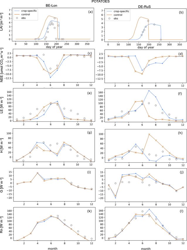
574                                                                      T. Boas et al.: Representing cropland sites in CLM5

many parts of the world (Urban et al., 2012; Challinor et al.,      Levis et al. (2012) and Chen et al. (2015) revealed signifi-
2014; Deryng et al., 2014; Rosenzweig et al., 2014; Tai et al.,     cant sensitivities of energy and carbon fluxes to biases in crop
2014; Levis et al., 2018), understanding the impact of climate      phenology, especially for the seasonality of the NEE for man-
change on crop production and improving its prediction at           aged crop sites where the flux is governed by planting and
local to global scales is a research topic of great importance      harvest times. In its latest version, CLM (CLM5) has been
to society. In addition, agricultural expansion and manage-         extended with an interactive crop module that represents crop
ment practices exert strong influences on physical and bio-         management. It includes eight actively managed crop types
geochemical properties of terrestrial ecosystems that need to       (temperate soybean, tropical soybean, temperate corn, tropi-
be considered in model simulations of the terrestrial system.       cal corn, spring wheat, cotton, rice, and sugarcane), as well as
Thus, the evaluation and improvement of integrated model-           irrigated and non-irrigated unmanaged crops (Lombardozzi
ing approaches, including through incorporation of improved         et al., 2020). CLM5 is the only land surface model to date
crop phenology, to simulate realistic land management and           that includes time-varying spatial distributions of major crop
crop yield in response to climate conditions are the focus of       types and their management (Lombardozzi et al., 2020). De-
many studies (Stehfest et al., 2007; Olesen et al., 2011; Van       spite these improvements over earlier versions of CLM, the
den Hoof et al., 2011; Rosenzweig et al., 2014).                    few studies that evaluated CLM5 at point and regional scales
   Nevertheless, the sophisticated representation of agricul-       suggest inaccurate phenology and crop yield estimates for
tural land cover in Earth system models (ESMs) remains an           specific crops (Chen et al., 2018; Sheng et al., 2018). In sum-
ongoing challenge due to the complexity of agricultural man-        mary, current crop modules in LSMs are limited by their abil-
agement decisions and the variety of different crop types and       ity to represent many different crop types and important man-
their respective phenologies. In many land surface models           agement practices such as cover cropping and flexible fertil-
(LSMs) and land components of ESMs, the representation              izer application types and amounts. The main challenges are
of crops is limited to simplistic schemes lacking the repre-        related to the complex parameterization of simulated crop va-
sentation of management (e.g., irrigation and fertilization) or     rieties due to their distinct phenology in combination with
to surrogate representation by natural grassland (Betts, 2005;      information scarcity, as well as the complexity of human in-
Elliott et al., 2015; McDermid et al., 2017). In recent studies     teraction through management decisions and biogeochemical
there is a trend towards the incorporation of a comprehen-          processes. In addition to irrigation and fertilizer application,
sive crop module in LSMs. These modules offer improved              crop rotations and cover cropping are important management
potential to study changes in water and energy cycles and           practices, and their consideration is a crucial factor to accu-
crop production in response to climate, environment, land           rately represent energy fluxes and crop phenology of agricul-
use, and land management changes. This may help to im-              tural sites (or areas) over longer timescales.
prove the simulation of biogeophysical and biogeochemical              In western Europe, a large proportion of arable land is cul-
processes on regional and global scales (Kucharik and Brye,         tivated with rotations of different non-perennial cash crops
2003; Lobell et al., 2011; Lokupitiya et al., 2009; Levis et al.,   (Kollas et al., 2015; Eurostat, 2018). The most important
2012; Osborne et al., 2015; McDermid et al., 2017; Lawrence         cash crops grown in the European Union (EU) are cereals,
et al., 2018; Lombardozzi et al., 2020). For example, the           such as wheat (mostly winter wheat varieties in Western Eu-
Simple Biosphere model (SiB) incorporated a crop module             rope), barley, and maize; root crops, such as sugar beet and
to represent a number of temperate crop varieties, which re-        potatoes; and oilseed crops, such as rapeseed, turnip rape-
sulted in improved simulated leaf area index (LAI) and net          seed, and sunflowers (Eurostat, 2018). Cereals account for
ecosystem exchange (NEE) (Lokupitiya et al., 2009). In ad-          the majority of all crop production in the EU, contribut-
dition, the Joint UK Land Environment Simulator (JULES)             ing up to 12 % to global cereal grain production (Eurostat,
was extended to a global representation of crops, which im-         2018). The EU production of sugar beet accounts for about
proved simulated LAI and gross primary production (GPP)             half of the global production (Eurostat, 2018). The use of
(Osborne et al., 2015).                                             cover crops is a common agricultural management practice
   Recent versions of the Community Land Model (CLM,                to reduce soil erosion, soil compaction, and nitrogen leach-
i.e., 4.0, 4.5, and 5.0) have adopted the prognostic crop mod-      ing and to increase agricultural productivity by nitrogen fix-
ule from the Agro-Ecosystem Integrated Biosphere Simula-            ation (Sainju et al., 2003; Lobell4 et al., 2006; Basche et al.,
tor (Agro-IBIS) (Kucharik and Brye, 2003), which has the            2014; Plaza-Bonilla et al., 2015; Tiemann et al., 2015; Kaye
ability to simulate the soil–vegetation–atmosphere system in-       and Quemada, 2017). The biogeochemical effects and bene-
cluding crop yields and has been evaluated in multiple stud-        fits of cover crops, as well as their potential to mitigate cli-
ies (e.g., Twine and Kucharik, 2009; Webler et al., 2012;           mate change, are the focus of many studies (e.g., Sainju et al.,
Xu et al., 2016). Even the simplified version of the Agro-          2003; Lobell et al., 2006; Groff, 2015; Plaza-Bonilla et al.,
IBIS crop scheme that was implemented in CLM4 led to                2015; Basche et al., 2016; Carrer et al., 2018; Lombardozzi
improved simulation of climate–crop interactions and more           et al., 2018; Hunter et al., 2019). Despite recent development
comprehensive ecosystem balances than previous CLM ver-             efforts, the representation of these management practices has
sions (Levis et al., 2012). Evaluation studies of CLM4 by           not yet been included in CLM5. Furthermore, in a previous

Geosci. Model Dev., 14, 573–601, 2021                                                 https://doi.org/10.5194/gmd-14-573-2021
T. Boas et al.: Representing cropland sites in CLM5                                                                            575

study by Lu et al. (2017) the default representation of win-          Vegetated land units are separated into natural vegetation
ter cereals performed poorly in simulating the phenology of        and crop land units, with only one crop functional type (CFT)
winter wheat.                                                      on each soil column, including irrigation as a CFT-specific
   In this study, we evaluate and enhance the performance of       land management technique (Lawrence et al., 2018; Lom-
the crop module of CLM5 focusing on the representation of          bardozzi et al., 2020). A total of 78 plant and crop functional
seasonal and inter-annual variations in crop growth, plant-        types are included in CLM5, including an irrigated and unir-
ing and harvesting cycles, crop yields, and energy and car-        rigated unmanaged C3 crop; 8 actively managed crop types
bon fluxes. Firstly, we transferred the modified vernalization     – spring wheat, temperate and tropical corn, temperate and
and cold-tolerance routine by Lu et al. (2017) to the CLM5         tropical soybean, cotton, rice, and sugarcane; and 23 crop
code to simulate winter cereal in a more meaningful way.           types without specific crop parameters associated with them
Secondly, new crop-specific parameter sets for winter wheat,       that are merged to the most closely related and parameter-
sugar beet, and potatoes that were gathered from the liter-        ized CFTs (Lombardozzi et al., 2020). For the simulation
ature and from observation data were added to the default          of those inactive crop types, the specific crop parameters of
parameter scheme. Finally, we extended CLM5 by adding a            the spatially closest and most similar out of the eight active
new crop rotation and cover-cropping subroutine that mod-          crop types are used. Irrigation is simulated dynamically for
els the growth of winter cover crops and the rotation from a       defined irrigated CFTs in response to soil moisture condi-
summer to a winter crop within the same year. All modifica-        tions and is partly based on the implementation of Ozdogan
tions were tested at the point scale at four cropland reference    et al. (2010) (Leng et al., 2013; Lawrence et al., 2018).
sites of the ICOS (Integrated Carbon Observation System)              Besides water availability from irrigation and precipi-
and TERENO (Terrestrial Environmental Observatory) net-            tation, crop yield and food productivity greatly depends
works in central Europe.                                           on fertilization. In CLM5-BGC-Crop, fertilization is repre-
                                                                   sented by adding nitrogen directly to the soil mineral pool
                                                                   (Lawrence et al., 2018). Fertilization dynamics and annual
2     Materials and methods                                        fertilizer amounts depend on the crop functional types and
                                                                   vary spatially and yearly based on the land use and land cover
2.1    Community Land Model                                        change time series derived from the Land Use Model Inter-
                                                                   comparison Project (Lawrence et al., 2019). In CLM5, land
Land surface models such as CLM5 are broadly applied               fractions with natural vegetation are not influenced by fertil-
in scientific studies to simulate water, energy, and nutri-        izer application. In cropping units, mineral fertilizer applica-
ent fluxes in the terrestrial ecosystem (Niu et al., 2011;         tion starts during the leaf-emergence phase of crop growth
Han et al., 2014; Lawrence et al., 2018; Naz et al., 2019).        and continues for 20 d. Manure nitrogen is applied at slower
CLM5 represents the latest version of the land component           rates (0.002 kg N m−2 yr−1 by default) to prevent rapid den-
in the Community Earth System Model (CESM) (Lawrence               itrification rates that were observed in earlier CLM versions
et al., 2018, 2019). In CLM5, simulated land surface fluxes        so that more uptake by the plant is achieved (Lawrence et al.,
such as latent and sensible heat are driven by atmospheric         2018).
and meteorological input variables in combination with                CLM5-BGC-Crop is fully prognostic with regards to car-
soil and vegetation states (e.g., soil moisture and LAI)           bon and nitrogen in the soil, vegetation, and litter at each
and parameters (e.g., hydraulic conductivity, land cover)          time step. The crop phenology and the carbon and nitrogen
(Oleson et al., 2010; Lawrence et al., 2011; Lawrence et           cycling processes follow three phenology phases: phase (1)
al., 2018). The new biogeochemistry and crop module of             from planting to leaf emergence, phase (2) from leaf emer-
CLM5 (BGC-Crop) adopted the prognostic crop module                 gence to beginning of grain fill, and phase (3) from beginning
from the Agro-Ecosystem Integrated Biosphere Simulator             of grain fill to maturity and harvest. These phenology phases
(Agro-IBIS) (Kucharik and Brye, 2003). This incorporation          are governed by temperature thresholds and the percentage
of agriculturally managed land cover may help to improve           of growing degree days (GDDs) required for maturity of the
the general representation of biogeochemical processes on          crop, with harvest occurring when maturity is reached (Lom-
the global scale to better address challenges from land use        bardozzi et al., 2020).
changes and agriculture practices (e.g., Lobell et al., 2006).        The first phenology stage, planting, starts when crop spe-
The CLM5 crop module includes new crop functional types,           cific 10 d mean temperature thresholds (of both the daily 2 m
updated fertilization rates and irrigation triggers, a transient   air temperature T10 d and the daily minimum 2 m air tem-
crop management option, and some adjustments to pheno-             perature Tmin,10 d ) are met. The transition from planting to
logical parameters. In addition, extensive modifications have      leaf emergence (phase 2) begins when the growing degree
been made to the grain C and N pool. For example, C for            days of soil temperature at 0.05 m depth (GDDTsoi ) reaches
annual crop seeding comes from the grain C pool, and ini-          1 %–5 % of the GDDs required for maturity (GDDmat ), de-
tial seed C for planting is increased from 1 to 3 gC m−2           pending on a crop-specific base temperature for the GDDTsoi .
(Lawrence et al., 2018, 2019; Lombardozzi et al., 2020).           Grain fill (phase 3) starts with either the simulated 2 m air

https://doi.org/10.5194/gmd-14-573-2021                                                 Geosci. Model Dev., 14, 573–601, 2021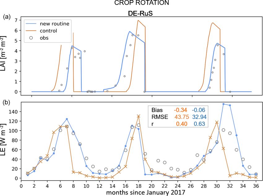
576                                                                      T. Boas et al.: Representing cropland sites in CLM5

temperature (GDDT2m ) reaching a heat unit threshold (h) of       tolerance (Barlow et al., 2015; Chouard, 1960). Vernaliza-
40 %–65 % of GDDmat or when the maximum leaf area in-             tion represents the process that an exposure to a period of
dex (Lmax ) is reached. The crop is harvested in one time step    nonlethal low temperatures is required to enter the flowering
when 100 % GDDmat is reached or when the crop-specific            stage for winter crops. In general, the vernalization process
maximum number of days past planting is exceeded. The             ensures that the reproductive development of plants growing
LAI is dependent on the specified specific leaf area (SLA)        over winter (winter crops and also natural vegetation) does
and the calculated leaf C. The SLA and the maximum LAI            not start in late summer or fall but rather in late winter or
are specified for each crop in the parameter file (Table A2).     spring. The other process, cold tolerance, ensures that the
   The allocation of carbon and nitrogen also follows the         crop can acclimate to low temperatures and thus survive cold
phenology phases. During the leaf-emergence phase, carbon         temperatures and even freeze–thaw cycles. However, cold
from the seed carbon pool is transferred to the leaf carbon       damage to the crop can occur when the crop is exposed to low
pool. Nitrogen is supplied through the soil mineral nitrogen      temperatures at a certain development stage. These damages
pool. During the grain-fill phases, nitrogen from the leaf and    have been documented to have significant impacts in crop
stem of the plant is translocated to the grain pool. Alloca-      yield (Lu et al., 2017). Lu et al. (2017) introduced a new ver-
tion ends upon harvest of the crop, when grain carbon and         nalization, as well as a cold-tolerance and frost damage sub-
nitrogen are transferred from the grain pool to the grain prod-   routine in CLM4.5 to better simulate the phenology of winter
uct pool and a small amount (3 gC m−2 ) is transferred to the     cereal. For this, they adapted the winter wheat vernalization
seed carbon pool for the next planting (Lawrence et al., 2018;    model from Streck et al. (2003). Streck et al. (2003) evalu-
Lombardozzi et al., 2020).                                        ated their vernalization algorithm for a wide range of winter
   The total amount of assimilated carbon and nitrogen is         wheat cultivars for the purpose of being used in crop model
regulated by availability of soil nitrogen, among other re-       approaches. Furthermore, Lu et al. (2017) implemented a
sources, and also depends on crop-specific target C/N ratios      cold-tolerance scheme that includes frost damage representa-
in the plant tissue (varying for roots, stem, leaves, reproduc-   tion using the approaches of Bergjord et al. (2008) and Vico
tive pools) (Lawrence et al., 2018; Lombardozzi et al., 2020).    et al. (2014). In this study, their modifications were ported to
For a detailed technical description of the model and all its     the newer version of the model, CLM5, and tested for several
features, the reader is referred to the technical documenta-      study sites.
tion and description of new features in CLM5 (Lawrence et            Vernalization and cold tolerance are cumulative processes
al., 2018, 2019; Lombardozzi et al., 2020).                       that operate in certain optimum temperature ranges (which
                                                                  can be different for different crop types and cultivars). The
2.2     Model modifications                                       vernalization process starts after leaf emergence and ends
                                                                  before flowering (Streck et al., 2003) and is dependent on
In the course of this study, three main limitations of CLM5       the crown temperature (Tcrown ) (see Eq. A1). The crown is
for the intended simulation of agricultural sites in western      the connecting tissue between the roots and the shoots at the
Europe at point scale were identified: (1) the default CLM5-      base of the plant. For winter wheat, the crown node is lo-
BGC-Crop code and parameterization yielded a very poor            cated at about 3–5 cm soil depth (Aase and Siddoway, 1979).
representation of crop growth of winter wheat and other win-      The daily vernalization dependence is calculated based on
ter crops, (2) the default plant parameter data set lacks spe-    Tcrown , and the optimum vernalization temperature (Topt ) is
cific parameterization for several important cash crops (here     limited to times when the crown temperature lies within the
sugar beet and potatoes in particular), and (3) CLM5-BGC-         minimum to maximum vernalization temperature (Tmin and
Crop does not allow a second crop growth onset or a second        Tmax ) range:
CFT to be grown on the same field within 1 year. These lim-              X
itations were resolved by modifications to the code structure     vd =       fvn (Tcrown ) ,                                  (1)
and parameterization of the CLM5-BGC-Crop module de-
                                                                  fvn (Tcrown ) =
scribed below.                                                                                   α
                                                                   2(Tcrown − Tmin )α Topt − Tmin − (Tcrown − Tmin )2α
2.2.1    Winter cereal representation                                                                                  , (2)
                                                                                      (Topt − Tmin )2α
                                                                                     ln 2
Winter wheat is an important crop for global food production      α=                                                     (3)
                                                                      ln[(Tmax − Tmin )/(Topt − Tmin )],
and covers a significant fraction of the European croplands
(Chakraborty and Newton, 2011; Vermeulen et al., 2012). In                   vd5
                                                                  vf =                                                        (4)
general, winter wheat is exposed to a different range of envi-           22.55 + vd5 ,
ronmental stresses compared to summer crops, such as low
temperatures. In regions with sufficiently cold winters, the      where vd (–) is the sum of the sequential vernalization days;
main processes that allow a successful cultivation of winter      fvn (–) is the daily vernalization rate; vf (–) is the vernal-
wheat during the colder months are vernalization and cold         ization factor; Tcrown (K) is the crown temperature; and Topt

Geosci. Model Dev., 14, 573–601, 2021                                                 https://doi.org/10.5194/gmd-14-573-2021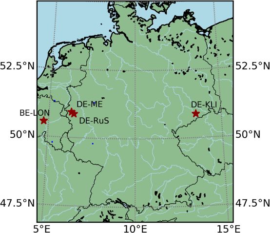
T. Boas et al.: Representing cropland sites in CLM5                                                                              577

(K), Tmax (K), and Tmin (K) are the optimum, maximum, and            crown temperature are low, the WDD will be high (Vico et
minimum vernalization temperatures, respectively.                    al., 2014).
   The vernalization factor can range between 0 (not ver-               Lu et al. (2017) also implemented a relationship between
nalized) and 1 (fully vernalized). It is multiplied with the         frost damage described above and the subsequent growth or
GDD value during the phenology phase after planting and              carbon allocation of the plant. Whenever the survival fac-
the grain carbon allocation coefficient, which leads to a re-        tor is less than 1, a small amount of leaf carbon (5 gC m−2
duced growth rate in the beginning of the phenology cycle            per model time step) and a small amount of leaf nitrogen
until the plant is fully vernalized. The vernalization factor        (scaled by the prescribed C/N target ratios; see Table 1 and
is further used in the cold-tolerance subroutine to assess the       Table A2) are transferred to the soil carbon and nitrogen litter
cumulative cold hardening of the plant and the dehardening           pool, thus simulating a reduction in growth and/or damage of
process when exposed to higher temperatures (see below).             small and young leaves and seedlings. Additionally, in order
Lu et al. (2017) introduced a scheme to quantify the impacts         to simulate more drastic and instantaneous damage or death
of frost damage based on the approaches following Bergjord           of the plant due to a longer duration of lethal temperatures
et al. (2008) and Vico et al. (2014). The damage from low            (most likely to occur in spring when the plant has emerged
temperatures is quantified by three main variables: the tem-         and is close to or already fully vernalized), a second frost
perature at which 50 % of the plant is damaged (LT50 ), the          damage function is implemented. When WDD > 1◦ d, the
survival probability (fsurv ), and winter killing degree days        frost damage function is triggered, leading to crop damage
(WDDs) (Bergjord et al., 2008; Lu et al., 2017; Vico et al.,         by transferring leaf carbon (amount scaled by the survival
2014). A detailed description of these approaches can be             probability (1 − fsurv )) to the soil carbon litter pool.
found in Bergjord et al. (2008) and Vico et al. (2014).                 A more detailed description of these routines can be found
   The temperature at which 50 % of the plant is damaged             in the source literature (Lu et al., 2017, and references
(LT50 ) is calculated interactively at each time step (LT50,t )      therein).
depending on the previous time step (LT50,t−1 ) and on sev-
eral accumulative parameters. These parameters are the ex-           2.2.2   Crop-specific parameterization
posure to near-lethal temperatures (rates ), the stress due to
respiration under snow (rater ), the cold hardening or low-          In order to yield a reasonable representation of agricultural
temperature acclimation (contribution of hardening, rateh ),         areas on the regional scale in future studies, the default pa-
and the loss of hardening due to the exposure to a period of         rameter set was extended with specific crop parameters for
higher temperatures (dehardening, rated ) that are each func-        sugar beet, potatoes, and winter wheat based on the char-
tions of the crown temperature (Lu et al., 2017, and refer-          acteristics of our study sites to better fit the observed plant
ences therein) (see Eqs. A2–A11).                                    phenology and energy fluxes at the simulation sites.
   The survival rate (fsurv ) is then calculated as a function of       The CFTs sugar beet and potatoes are merged to the spring
LT50 and the crown temperature. The probability of survival          wheat CFT on the default parameter scheme due to the
is a function of Tcrown in time (t). It increases once Tcrown is     lack of crop-specific parameters for these crops. For win-
higher than LT50 and decreases when it is lower than LT50            ter wheat there is a preexisting default parameter set avail-
(Vico et al., 2014):                                                 able in CLM5. However, this default parameterization per-
                                αsurv
                                                                     formed poorly in representing the crop phenology for the
                     − TLT
                        crown
                                                                     evaluated study sites in this study. This was also reported
fsurv (Tcrown , t) = 2    50            ,                     (5)
                                                                     in an earlier study by Lu et al. (2017). Thus, crop-specific
where αsurv is a shape parameter of 4.                               parameters were added for sugar beet, potatoes, and winter
   The winter killing degree day (WDD) is calculated as              wheat. The parameters to be modified were selected taking
a function of crown temperature and survival probability,            into account the sensitivity analysis and parameter estima-
where the maximum function limits the integration to the po-         tion studies by Post et al. (2017) (for version 4.5), Cheng et
tentially damaging periods and when the air temperature (T )         al. (2020), and Fisher et al. (2019) (for version 5.0). Key pa-
is lower than the base temperature (Tbase ) of 0 ◦ C (Vico et al.,   rameters as identified by previous studies (Sulis et al., 2015;
2014):                                                               Post et al., 2017; Lu et al., 2017; Fisher et al., 2019; Cheng et
                                                                     al., 2020) are listed in Table 1. These parameters were added
           Z
                                                                     with values from the literature or site-specific observations to
WDD =          max[(Tbase − Tcrown ), 0]
                                                                     match observed values. General phenology parameters such
          winter                                                     as the maximum canopy height, planting temperatures, max-
  [1 − fsurv (Tcrown , t)]dt.                                 (6)    imum LAI, maximum and minimum planting dates, and days
                                                                     for growing were adjusted according to field data, including
Lower LT50 indicates a higher frost tolerance and would re-          planting and harvest dates. A list of plant types and plant-
sult in higher survival rates, smaller WDD, and less cold            ing and harvest dates is provided in Table A1. C/N ratios in
damage to the plant. Thus, when the survival probability and         leaves and roots for wheat and sugar beet were adapted from

https://doi.org/10.5194/gmd-14-573-2021                                                   Geosci. Model Dev., 14, 573–601, 2021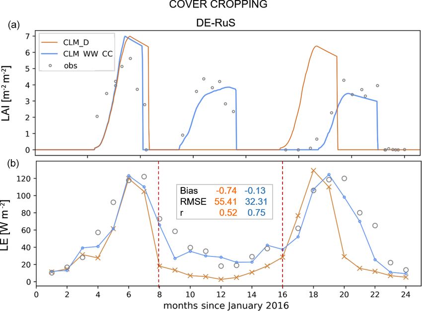
578                                                                           T. Boas et al.: Representing cropland sites in CLM5

Table 1. CFT-specific phenology, carbon and nitrogen ratios, and allocation parameters.

              Parameter                                                      CLM variable name         Units
              Phenology
              Minimum planting date for the Northern Hemisphere              min_NH_planting_date      MM.DD
              Maximum planting date for the Northern Hemisphere              max_NH_planting_date      MM.DD
              Average 5 day daily temperature needed for planting            planting_temp             K
              Average 5 d daily minimum temperature needed for planting      min_planting_temp         K
              Minimum growing degree days                                    gddmin                    ◦d
              Maximum number of days to maturity                             mxmat                     Days
              Growing degree days for maturity                               hygdd                     ◦d
              Base temperature for GDD                                       baset                     ◦C
              Maximum temperature for GDD                                    mxtmp                     ◦C
              Percentage of GDD for maturity to enter phase 3                lfemerg                   % GDDmat
              Percentage of GDD for maturity to enter phase 4                grnfill                   % GDDmat
              Canopy top coefficient                                         ztopmax                   M
              Maximum leaf area index                                        laimx                     m2 m−2
              Specific leaf area                                             slatop                    m2 gC−1
              CN ratios and allocation
              Leaf C/N                                                       leafcn                    gC gN−1
              Minimum leaf C/N                                               leafcn_min                gC gN−1
              Maximum leaf C/N                                               leafcn_max                gC gN−1
              Fine root C/N                                                  frootcn                   gC gN−1
              Grain C/N                                                      graincn                   gC gN−1
              Fraction of leaf N in RuBisCo                                  flnr                      fraction per gNm−2

Whitmore and Groot (1997), Gan et al. (2011), Sánchez-                  when representing ecosystems where agricultural manage-
Sastre et al. (2018), and Zheng et al. (2018). The specific             ment practices involve multiple sowing and harvest cycles
leaf area (slatop) and the fraction of leaf N in RuBisCo (flnr)         in accordance with the monsoon season (e.g., India). There-
for sugar beet and winter wheat were taken from Sulis et                fore, a cover-cropping subroutine was implemented in the
al. (2015) and references therein and also adopted for pota-            BGC phenology module that affects the onset–offset (crop
toes.                                                                   cycle/fallow) algorithm to allow a second onset period (crop
   Table A2 provides a full list of default and newly added             cycle) on the same column.
crop-specific parameters for the CFTs temperate corn, spring               A cover crop flag was introduced in the parameter file and
wheat, sugar beet, potatoes, and winter wheat.                          in the source code. This flag can be set for any CFT in the
                                                                        parameter file and calls the cover-cropping subroutine when
2.2.3   Cover-cropping and crop rotation scheme                         it is set to true (covercrop_flag 6 = 0). This allows a flexible
                                                                        handling of this option and for its application on a larger
The effect of cover crops on the physical and biogeochemical            scale. With this modification, the onset period can start again
properties of the land surface alters latent heat flux, albedo,         within 1 simulation year for another (or the same) CFT. For
and soil carbon and nitrogen storage and can potentially im-            example, when the maturity of the crop is reached and it has
pact local and regional climate (Sainju et al., 2003; Lobell            been harvested, the model would by default switch to the next
et al., 2006; Möller and Reents, 2009; Plaza-Bonilla et al.,            stage (phase 4), where the crop is not alive and the offset
2015; Basche et al., 2016; Carrer et al., 2018; Lombardozzi             (fallow) period begins. The next onset period and GDD ac-
et al., 2018; Hunter et al., 2019).                                     cumulation for planting would then start in the subsequent
   In the default BGC phenology, the growth algorithm starts            simulation year. In our modified CLM5 version, the cover-
in the beginning of each year, when the crop is not alive on            cropping subroutine is called before entering into the offset
the specific patch. Furthermore, the CLM structure does not             period when the cover-crop flag for the current CFT is set
allow multiple CFTs to coexist on the same column so that               to true. In the cover-cropping subroutine, the CFT is then
multiple planting phases related to cover cropping over win-            changed according to a predefined rotation scheme, and an-
ter months or crop rotations with winter and summer crops,              other onset period and GDD accumulation for planting is ini-
both being very common practices in Europe and world-                   tialized.
wide, cannot be accounted for. This might also be an issue

Geosci. Model Dev., 14, 573–601, 2021                                                     https://doi.org/10.5194/gmd-14-573-2021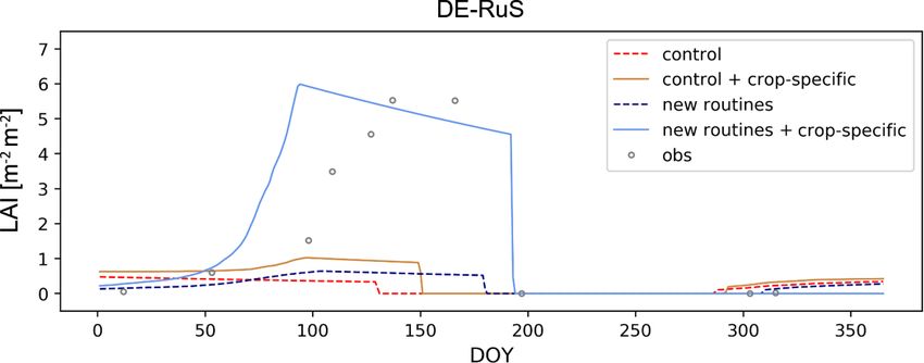
T. Boas et al.: Representing cropland sites in CLM5                                                                           579

   A common practice is to plow the cover crops into the soil
instead of removing their biomass from the field. We simu-
lated this by relocating the biomass of the crop into the litter
pool instead of the grain product pool upon harvest using the
use_grainproduct flag described below (Eq. 7).
   Individual crop rotation schemes were customized within
the code and depend on the currently planted crop type. For
example, if a simulation starts with a crop coverage of spring
wheat specified in the surface file, the new subroutine is
called after harvest of the crop. Within the subroutine, the
CFT is then changed to the next crop, e.g., sugar beet. Af-
ter the harvest of this crop, e.g., sugar beet, the CFT is again
changed to the next crop and so on. When the CFT is changed
back to spring wheat, the rotation cycle starts again. This ro-
tation is defined in a repetitive sequence based on the har-
vested CFT and its harvest date:

if harvdate (p) ≥ hd1 and ivt(p) = crop1 then
       ivt(p) = crop2                                               Figure 1. ICOS and TERENO cropland study sites Selhausen
       croplive(p) = false                                          (DE-RuS), Merzenhausen (DE-RuM), Klingenberg (DE-Kli), and
                                                                    Lonzée (BE-Lon).
       idop(p) = not_planted
       use_grainproduct = true
else if harvdate (p) ≥ hd2 and ivt(p) = crop2 then                  2.3   Study sites and validation data
       ivt(p) = crop3
                                                                    The CLM5 model was set up for four European cropland
       croplive(p) = false
                                                                    sites: Selhausen, Merzenhausen, Klingenberg, and Lonzée
       idop(p) = not_planted                                        (Fig. 1). These sites were selected mainly for their excellent
       use_grainproduct = true,                              (7)    continuous measurements of surface energy fluxes.
                                                                       Selhausen (50.86589◦ N, 6.44712◦ E) is part of the
where harvdate is the harvest day of the current simulation         TERENO Rur Hydrological Observatory (Bogena at al.,
year, hd is the customizable harvest date of the respective         2018) and the Integrated Carbon Observation System (ICOS,
CFT, p is the simulated patch on the model grid, ivt is the         2020). The test site covers an area of approximately
simulated CFT, crop1−3 represent the user-specified CFTs to         1 km × 1 km and is located in the catchment of the Rur river
the rotated, idop is the planting day, and use_grainproduct is      (Bogena et al., 2018). Selhausen had a crop rotation of sugar
a flag to define whether the grain carbon of simulated crop is      beet (Beta vulgaris), winter wheat (Triticum aestivum), and
to be harvested into the food pool or not. If this flag is set to   winter barley (Hordeum vulgare) and also less frequently
false, the plant carbon and nitrogen are transferred to the soil    featured rapeseed (Brassica napus) and potatoes (Solanum
litter pool and not allocated to the food product pool upon         tuberosum) from 2015 to 2019. Cover crops such as oilseed
harvest of the crop.                                                radish or cover crop mixes are planted occasionally between
    The actual rotation of crop types can be customized by the      two main crop rotations. Continuous records of meteorolog-
user by defining the variables hd and cropx in a list (e.g.,        ical variables, soil-specific observations, and greenhouse gas
hd1 = 150 [day of year], crop1 = spring wheat). By includ-          and energy fluxes have been available for Selhausen since
ing the harvest date as a dependency, it is also possible to        2011. Regular LAI measurements have been available since
simulate the planting of cover crops based on harvest date          2016 (Ney and Graf, 2018).
thresholds. A user-defined maximum harvest date for any                Merzenhausen (50.93033◦ N, 6.29747◦ E) is located at ap-
specific cash crop can define whether a cover crop would be         proximately 14 km from Selhausen and is also part of the
planted or not. This technique can be beneficial to study the       TERENO Rur Hydrological Observatory. The crop rotation
effects of conceptual cover-cropping scenarios on regional          of the site includes sugar beet (Beta vulgaris), winter wheat
scales. The possibility to change the CFT within the same           (Triticum aestivum), winter barley (Hordeum vulgare), rape-
year represents a significant improvement in flexibility, as        seed (Brassica napus), and occasionally catch cover crop
CLM5 only permitted land use changes at the beginning of            mixes. For Merzenhausen, continuous records of meteo-
every year. In order to simulate cover cropping at our study        rological variables, soil-specific observations, and energy
site DE-RuS, we implemented a new CFT for a greening mix            fluxes have been available since 2011. Regular LAI measure-
cover crop (or covercrop1 ).                                        ments were available from 2016 to 2018.

https://doi.org/10.5194/gmd-14-573-2021                                                 Geosci. Model Dev., 14, 573–601, 2021
580 T. Boas et al.: Representing cropland sites in CLM5 Klingenberg (50.89306◦ N, 13.52238◦ E) is an ICOS crop- Site-specific measurement records of latent and sensible land site located in the mountain foreland of the Erzgebirge heat fluxes, net ecosystem exchange (NEE), LAI, soil tem- that is operated by the Technical University Dresden (TU perature, and soil moisture were used as validation data for Dresden) (ICOS, 2020; Prescher et al., 2010). The site is the simulation runs. characterized as managed cropland with a 5-year planting ro- Forcing variables were always used in gap-filled form, tation of rapeseed (Brassica napus), winter wheat (Triticum while validation variables were used in unfilled, quality- aestivum), maize (Zea mays), and spring and winter barley filtered form. (Hordeum vulgare) (Kutsch et al., 2010). Since 2004, data on ecosystem fluxes (including net ecosystem and net biome productivity), meteorological variables, and soil observations 3 Experimental design and analyses have been collected. Furthermore, biomass observations and agricultural management information are available for this 3.1 Model implementation site. The cropland site Lonzée (50.553◦ N, 4.746◦ E) in Bel- For the single-point study sites, CLM was run in point mode gium is also part of ICOS (Buysse et al., 2017). It has with only one grid cell and forced with site-specific hourly been planted in a 4-year rotation cycle with sugar beet meteorological data. The annual fertilization amounts at the (Beta vulgaris), winter wheat (Triticum aestivum), and potato single-point study sites were adjusted according to docu- (Solanum tuberosum) since 2000, with mustard as a cover mented amounts of applied fertilizer that ranged between crop after winter wheat harvest (Moureaux, 2006; Moureaux 12 and 20 gN m−2 . In CLM5, the potential photosynthetic et al., 2008). For Lonzée, continuous records of meteorolog- capacity and the total amount of assimilated carbon during ical variables, EC flux data, and LAI (GLAI and GAI) mea- the phenology stages are regulated by the availability of soil surements are available from 2004 onwards. General infor- nitrogen (Lawrence et al., 2018). With modern fertilization mation on the ICOS study sites, such as climatic conditions practices in Europe, nitrogen is not assumed to be a limiting and soil types, is provided on the ICOS Carbon Portal under factor for the studied sites. the respective site codes (ICOS, 2020). In order to balance ecosystem carbon and nitrogen pools, At all sites, the application of mineral fertilizer and herbi- gross primary production and total water storage in the sys- cides or pesticides, as well as occasional application of or- tem, a spin-up is required (Lawrence et al., 2018). An ac- ganic fertilizer, is regular management practice. celerated decomposition spin-up of 600 years and an addi- Station data required to force CLM, i.e., meteorological tional spin-up of 400 years was conducted for each site with variables (see the following section), were measured as block the BGC-Crop module (Lawrence et al., 2018; Thornton and averages over 10 min or at higher resolutions and gap-filled Rosenbloom, 2005). The simulated conditions at the end of using linear statistical relations to nearby stations where the spin-up were then used as initial conditions for the fol- possible (Graf, 2017) or by marginal distribution sampling lowing simulations. within the software package REddyProc otherwise (Wutzler In order to test the winter wheat representation, several et al., 2018). Fluxes required for model validation (i.e., net simulations were conducted for all winter wheat years at the ecosystem CO2 exchange (NEE), latent heat flux (LE), sen- sites DE-RuS, DE-RuM, DE-Kli, and BE-Lon. In a first step, sible heat flux (H ), soil heat flux (G), and gross primary pro- the impact of each modification was assessed individually duction (GPP)) and net radiation (Rn) were either measured by simulating one winter wheat year at the site DE-RuS us- (G and Rn) or computed from turbulent raw measurements ing four different model configurations: (1) the default model (frequency ≥ 10 s−1 ) using the eddy covariance method for and default parameter set (control), (2) the default model 30 min block averages by the respective site operators. Sub- with the new parameter set (control + crop-specific), (3) sequently, gaps were filled and GPP was estimated from NEE the extended winter wheat model with the default param- using REddyProc (Wutzler et al., 2018). More details on eter set (new routine), and (4) the extended winter wheat quality control, filling of longer gaps and by nearby stations, model with the new parameter set (new routine + crop- correction of soil heat flux, and energy balance closure anal- specific). Further evaluations for the other study sites and ysis are given in Graf et al. (2020), and these data sets are years were conducted for the combined winter wheat modifi- specifically given for DE-RuS and DE-RuM, including LAI cations CLM_WW (extended model with winter wheat sub- measurements, in Reichenau et al. (2020).The long-term an- routines and new crop-specific parameterization) in compar- nual energy balance closures of the sites DE-RuS, DE-Kli, ison to control simulations (default model configuration and and BE-Lon were approximately 79 %, 77 %, and 76 %, re- default parameterization of winter wheat). spectively, according to analyses in Graf et al. (2020), and For the evaluation of the crop-specific parameter sets for 76 % at DE-RuM according to an earlier study by Eder et sugar beet and potatoes, simulations were run with the new al. (2015). All half-hourly meteorological and flux data were parameterizations at the sites DE-RuS and BE-Lon over sev- aggregated to hourly averages to match our customized CLM eral years. For both sites, control simulations were conducted forcing time step. without the new parameter set, in which both CFTs sugar Geosci. Model Dev., 14, 573–601, 2021 https://doi.org/10.5194/gmd-14-573-2021
T. Boas et al.: Representing cropland sites in CLM5 581
beet and potatoes are simulated as a spring wheat by default. (control), the default model with the new parameter set (con-
Furthermore, an evaluation of the default parameterization trol + crop-specific), the extended winter wheat model with
for the CFT temperate corn at the site DE-Kli is included in the default parameter set (new routines), and the extended
the Supplement (Fig. S1, Table S1). winter wheat model with the new parameter set (new rou-
The cover-cropping and crop rotation scheme was tested tines + crop specific).
for two practical cases at DE-RuS. From 2016 to 2017, Using only the new crop-specific parameter set with the
planting was altered at DE-RuS from barley (here repre- default model configuration resulted in slightly higher LAI
sented by the CFT for spring wheat) in 2016 to sugar beet values compared to the control run but did not reach the ob-
in 2017 with a greening mix cover crop in between (win- served maximum LAI values and the growth cycle duration.
ter months 2016/2017). In order to simulate this common The implementation of the winter wheat subroutines using
cover-cropping practice, we implemented a new CFT for a the default parameter set led to a more realistic reproduction
greening mix cover crop (or covercrop1 ). For the years 2017 of the growth cycle duration compared to the control run but
to 2019 at DE-RuS, the subroutine’s ability to simulate re- did not yield good correspondence with observed LAI mag-
alistic crop rotation cycles was tested by changing the sim- nitudes. The combination of the new crop-specific parameter
ulated CFT from sugar beet (2017) to winter wheat (2017– set and the new winter wheat subroutines resulted in the most
2018) and then to potatoes (2019). In this step, simulations realistic LAI dynamics (Fig. 2). As previously described by
were run with the previously tested crop-specific parameter- Lu et al. (2017), the default vernalization routine reaches a
izations for sugar beet, potatoes, and winter wheat. Simula- factor of 1 (fully vernalized) shortly after planting when the
tion results were again compared to a control simulation run, first frost occurs. This induced an unrealistically early com-
where a consecutive growth of spring wheat is simulated. mencement of the grain-fill stage within 2 months after plant-
ing in the control run (November or December). The default
3.2 Evaluation of model performance vernalization also resulted in peak LAI occurring too early in
the year, leading to significantly lower photosynthesis com-
For statistical evaluation of the model results, the root-mean- pared to the observations. This also applies to the implemen-
square error (RMSE), the bias (BIAS), and the Pearson cor- tation of the new crop-specific parameter set, which generally
relation (r) were chosen as performance metrics: leads to slightly higher LAI values.
v In the extended winter wheat model, the adapted vernal-
u n
u1 X ization routine produces lower initial vernalization factors,
RMSE = t (Xi − Xobs,i )2 , (8) which reduce the growing degree days. This leads to later
n i=1
onset of the leaf-emergence and grain-fill stage and allows
n n
X .X a more realistic representation of the LAI cycle and peak in
BIAS = (Xi − Xobs,i ) (Xobs,i ), (9) combination with the new crop-specific parameterization.
i=1 i=1
! In further evaluations, the combined winter wheat pack-
n
1 X age, including the new crop-specific parameterization and
r= Xobs,i − µobs ) · (Xi − µsim
n i=1
the extended winter wheat subroutines, is implemented
in CLM_WW simulations and compared to control runs
/(σsim · σobs ), (10) (Fig. 3). For all study sites and simulation years, CLM_WW
simulations resulted in a much better representation of the
where i is time step and n the total number of time steps. Xi
growth cycle and corresponding seasonal LAI variation and
and Xobs,i are the simulated and the observed values at ev-
magnitudes compared to control simulations (Fig. 3). In ad-
ery time step, with µsim and µobs being the respective mean
dition, the temporal pattern of energy fluxes and NEE were
values. The standard deviation of simulation results and mea-
improved with CLM_WW compared to the control run.
surement data are represented by σsim and σobs , respectively.
In general, CLM_WW yielded LAI peak magnitudes sim-
The statistical evaluation was conducted for daily simula-
ilar to observations at the sites BE-Lon, DE-RuS, and DE-
tion output and daily observation data for the variables NEE,
RuM (Fig. 3). For DE-Kli, site-specific observations of the
LE, H , and Rn.
LAI were not available, but simulated LAI magnitudes for
DE-Kli using CLM_WW are similar to those for BE-Lon.
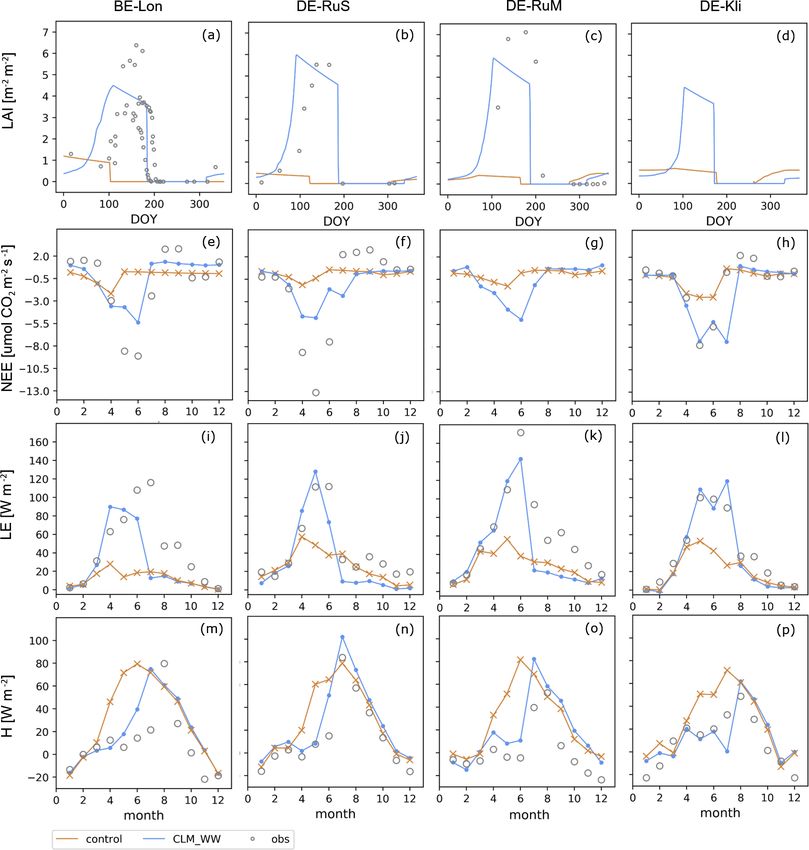
4 Results For the BE-Lon site, CLM_WW-simulated peak LAI magni-
tudes are close to the observations. An exception is the year
4.1 Winter cereal representation 2015, where CLM_WW underestimated the unusually high
LAI values observed in May and June, which ranged from
The impact of the new winter-wheat-specific parameteriza- 5.40 to 6.38 m2 m−2 . For BE-Lon, faster growth was simu-
tion and the new winter wheat routine, as well as the com- lated in the early growing stage of winter wheat, resulting in
bination of both, is illustrated in Fig. 2. Here we show sim- a more gradual increase in LAI compared to the other sites
ulated LAI for the default model and default parameter set (Fig. 3). This is related to higher air temperatures at BE-Lon
https://doi.org/10.5194/gmd-14-573-2021 Geosci. Model Dev., 14, 573–601, 2021582 T. Boas et al.: Representing cropland sites in CLM5 Figure 2. Daily simulation results for the LAI, simulated with default model and the default parameter set (control), the default model with new parameter set (control + crop-specific), the extended winter wheat model with default parameterization (new routines), and the extended model with the new parameter set (new routines + crop-specific), compared to point observations for a winter wheat year at DE-RuS. early in the growing stage (especially in February) that en- tion coefficients for the energy fluxes (LE, H and Rn) calcu- abled more simulated growth compared to the other sites. lated over the period from planting to harvest date for daily Overall, the LAI peak simulated with CLM_WW occurred simulation results and daily observation data improved for about 1 month earlier than observed, suggesting that mat- all sites (Table 4). The highest correlations were reached for uration was reached too early. This is also reflected in the the sites DE-Kli with r values of 0.62 and 0.71 and for BE- simulated CLM_WW harvest dates that are approximately Lon with r values of 0.5 and 0.46 for sensible heat and latent 1 month earlier than the recorded dates (Table 3). While heat flux, respectively (Table 4). Due to the simulated LAI the planting date is the same for the control run and the peak being too early, latent heat flux is underestimated by CLM_WW simulations, CLM_WW generally resulted in a CLM_WW (Fig. 3, Table 4). The high latent heat fluxes mea- better match of simulated and recorded harvest dates (1.5 to sured at BE-Lon and DE-Kli in the later months of the year 2 months later than control run). (from day 220 onwards) reflect the growth of a cover crop. The correlation of simulated grain yield and site records At both the BE-Lon site and at the DE-Kli site, cover crops was significantly improved by up to 87 % in CLM_WW sim- are typically sown after harvest of winter wheat (mustard at ulations compared to the control run. At the DE-RuS site, BE-Lon, radish and brassica at DE-Kli), and they strongly CLM_WW resulted in a grain yield of 9.15 t ha−1 that is very affect surface energy fluxes later in the year. In contrast, in close to the observed value of 9.2 t ha−1 , while grain yield the control simulations and CLM_WW, the crop fields were is strongly underestimated in the control run (1.17 t ha−1 ). simulated as fallow after the harvest of winter wheat (Fig. 3, For DE-Kli, the CLM_WW-simulated crop yield matched Table A1). While the correlation of the latent and sensible the recorded yield data very well for the year 2016 and was heat flux during the growing cycle of the crop is generally overestimated for 2011 by approximately 16 %. The control increased with the CLM_WW model, the overall annual cor- run resulted in an underestimation of yield by more than 80 % relation is still relatively poor due to the influence of cover (Fig. 4, Table 3). For BE-Lon the simulated crop yield is un- cropping and poor representation of post-harvest field condi- derestimated compared to site harvest records (Fig. 4, Ta- tions (annual performance metrics are included in the Sup- ble 3). While CLM_D simulations underestimated the grain plement, Table S3). Furthermore, CLM_WW was generally yield by approximately 85 %–90 %, CLM_WW underesti- better able to match NEE observations compared to control mated yield by only 18 %–36 % at BE-Lon. The simulated runs, partly due to the better representation of the seasonal yields by CLM_WW for the individual years show only min- LAI variations (Fig. 3). During the growing season of win- imal variations with values from 8.12 to 8.16 t ha−1 , while ter wheat, the negative peak in NEE coincides with the peak the measured yields ranged from 9.92 to 12.88 t ha−1 , indi- in LAI. Negative NEE values indicate a carbon sink and hap- cating that CLM did not capture the inter-annual yield varia- pen when the crop gains more carbon through photosynthesis tion very well (Table 3). than is lost through respiration. Correlation improved (com- Overall, the better representation of the winter wheat paring CLM_WW to the control run) from 0.13 to 0.46 for growing cycle by CLM_WW can also be inferred from the BE-Lon, from 0.21 to 0.33 for DE-RuS and from 0.29 to 0.56 simulated surface energy fluxes (Fig. 3). In terms of net ra- for DE-Kli. The resulting correlation for CLM_WW simula- diation, both CLM_WW and the control run are very close tions is still relatively low due to an underestimation of the to the observations (Table 4). However, CLM_WW was able cumulative monthly NEE during seasons with high NEE at to better capture seasonal variations of surface energy fluxes BE-Lon and DE-RuS. For DE-Kli, CLM_WW was able to during the growing cycle of the crop (Fig. 3). The correla- match NEE observed at peak LAI very well, but late sea- Geosci. Model Dev., 14, 573–601, 2021 https://doi.org/10.5194/gmd-14-573-2021
T. Boas et al.: Representing cropland sites in CLM5 583
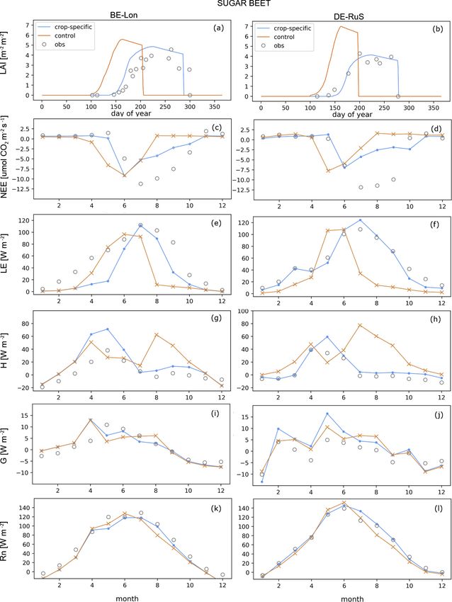
Figure 3. Simulation results of (a–d) LAI, and simulation results averaged for each month of (e–h) NEE, (i–l) LE, and (m–p) H for all winter
wheat years (see Table 3) at the sites (from left to right) BE-Lon, DE-RuS, DE-RuM, and DE-Kli. Simulation results from the new routine
with crop-specific parameterization (CLM_WW; blue) are compared to control simulations (orange) and available site observations (grey) of
LAI (all available point observations plotted) and fluxes (averaged over all respective years and for each month, respectively). Corresponding
performance statistics for daily simulation results during the crop growth cycle are listed in Table 4.
sonal NEE (July) shortly before harvest is overestimated by 4.2 Crop-specific parameterization of sugar beet and
CLM_WW, resulting in a low overall agreement with ob- potatoes
servation data. Furthermore, post-harvest field observations
at BE-Lon, DE-RuS, and DE-Kli indicate that heterotrophic The crop-specific parameter sets were tested for several years
respiration from soil organic matter and litter results in a car- with sugar beet and potato planting at BE-Lon and DE-RuS,
bon source that is not simulated well in CLM (no GPP, near- respectively. The performance in reproducing seasonal vari-
zero NEE) (Fig. 3). This poor representation of post-harvest ations and magnitudes of energy fluxes was strongly im-
field conditions is reflected in low correlations over the whole proved with the crop-specific parameterization. Correspond-
year (Table S3). ingly, simulations with the crop-specific parameter sets for
both sugar beet and potatoes were able to reasonably capture
seasonal variations and peak values of LAI and growth cycle
https://doi.org/10.5194/gmd-14-573-2021 Geosci. Model Dev., 14, 573–601, 2021584 T. Boas et al.: Representing cropland sites in CLM5
∗ Reference periods are 1961–2010 for DE-RuS (adapted also for DE-RuM), 2005–2019 for DE-Kli, and 2004–2017 for BE-Lon.
(T ), mean annual precipitation amounts (P ), and reference. Textural fractions for the top soil layers (up to 50 cm) at each study site are provided in Table A3.
Table 2. ICOS and TERENO cropland study site location coordinates and altitude (Alt.), soil types, Köppen–Geiger climate classification (Peel et al., 2007), mean annual temperature
Lonzée
Klingenberg
Merzenhausen DE-RuM
Selhausen
Site ID
DE-RuS
BE-Lon
DE-Kli
ICOS
ICOS
TERENO
TERENO ICOS
Project
50.553◦ N, 4.746◦ E
50.893◦ N, 13.522◦ E
50.930◦ N, 6.297◦ E
50.865◦ N, 6.447◦ E
Location
Figure 4. Annual grain yield (tDM ha−1 ) simulated with the con-
trol run (orange) and the extended winter wheat model with crop-
specific parameterization (blue), compared to recorded harvest
yields (grey) for all simulated winter wheat years (indicated on the
x axis) at the sites BE-Lon, DE-RuS, DE-RuM, and DE-Kli.
(m.s.l.)
104.5
Alt.
167
478
100
Luvisol
Gleysoil
Cambisol
Luvisol
type
Soil
length and harvest time (Figs. 5, 6). The control run in CLM
uses the spring wheat parameterization for these crop types
and therefore reproduced the growth cycle and seasonal LAI
Cfb – temperate maritime
Cfb – suboceanic, subcontinental
Cfb – temperate maritime
Cfb – temperate maritime
Climate
of spring wheat, while simulations using the crop-specific
potato and sugar beet parameterizations better captured har-
vest date and growth cycle of these crops.
The improved growth cycle representation with crop-
specific parameters also led to more accurate simulation of
energy fluxes. For sugar beet at BE-Lon, the latent heat flux
at peak LAI corresponds well with observed values while be-
ing underestimated before and after peak LAI, and hence the
sensible heat flux is overestimated at these times (Fig. 5).
Seasonal variations of energy fluxes and magnitudes were
(◦ C)∗
8.1
9.9
9.9
10
also captured much better in simulations with the new pa-
T
rameterization. The simulations with crop-specific parame-
(mm a−1 )∗
ters show slightly better net radiation correlations for both the
sugar beet and potato CFTs at each site, compared to the con-
800
766
698
698
P
trol run (Table 5). The correlation between simulated and ob-
served latent heat flux for sugar beet was strongly improved
Buysse et al.(2017)
Thomas Grünwald (personal communication, 2020)
Bogena et al. (2018)
Ney (2019)
Ref.
by changing the parameters (0.11 to 0.55 for DE-RuS and
0.21 to 0.55 for BE-Lon). The same is true for the simulated
sensible heat flux for sugar beet (0.04 to 0.76 for DE-RuS and
0.08 to 0.51 for BE-Lon). The NEE for the sugar beet CFT is
underestimated during peak LAI periods in the control run,
resulting in poorer correlations compared to latent and sensi-
ble heat flux and net radiation (Fig. 5). Simulations with the
crop-specific parameter set resulted in a reduction in negative
bias for NEE and reached higher correlation compared to the
control simulation (0.03 to 0.37 for DE-RuS and 0.05 to 0.64
for BE-Lon).
Similar improvements can be observed for the new potato
parameterization, while the correlation of simulation results
with observation data is generally lower compared to the
Geosci. Model Dev., 14, 573–601, 2021 https://doi.org/10.5194/gmd-14-573-2021You can also read