Benchmarking and Survey of Explanation Methods for Black Box Models
←
→
Page content transcription
If your browser does not render page correctly, please read the page content below
Benchmarking and Survey of Explanation Methods for
                                                               Black Box Models

                                         Francesco Bodria1 , Fosca Giannotti2 , Riccardo Guidotti3 , Francesca Naretto1 , Dino Pedreschi3 ,
                                                                            and Salvatore Rinzivillo2
                                                              1
                                                                  Scuola Normale Superiore, Pisa, Italy, {name.surname}@sns.it
                                                                     2
                                                                       ISTI-CNR, Pisa, Italy, {name.surname}@isti.cnr.it
                                                              3
                                                                  Largo Bruno Pontecorvo, Pisa, Italy, {name.surname}@unipi.it

                                                 Abstract. The widespread adoption of black-box models in Artificial Intelligence has en-
                                                 hanced the need for explanation methods to reveal how these obscure models reach specific
                                                 decisions. Retrieving explanations is fundamental to unveil possible biases and to resolve
                                                 practical or ethical issues. Nowadays, the literature is full of methods with different explana-
                                                 tions. We provide a categorization of explanation methods based on the type of explanation
                                                 returned. We present the most recent and widely used explainers, and we show a visual
arXiv:2102.13076v1 [cs.AI] 25 Feb 2021

                                                 comparison among explanations and a quantitative benchmarking.

                                         Keywords: Explainable Artificial Intelligence, Interpretable Machine Learning, Transparent Mod-
                                         els

                                         1     Introduction
                                         Today AI is one of the most important scientific and technological areas, with a tremendous
                                         socio-economic impact and a pervasive adoption in many fields of modern society. The impressive
                                         performance of AI systems in prediction, recommendation, and decision making support is generally
                                         reached by adopting complex Machine Learning (ML) models that “hide” the logic of their internal
                                         processes. As a consequence, such models are often referred to as “black-box models” [59,47,95].
                                         Examples of black-box models used within current AI systems include deep learning models and
                                         ensemble such as bagging and boosting models. The high performance of such models in terms
                                         of accuracy has fostered the adoption of non-interpretable ML models even if the opaqueness of
                                         black-box models may hide potential issues inherited by training on biased or unfair data [77].
                                         Thus there is a substantial risk that relying on opaque models may lead to adopting decisions that
                                         we do not fully understand or, even worse, violate ethical principles. Companies are increasingly
                                         embedding ML models in their AI products and applications, incurring a potential loss of safety
                                         and trust [32]. These risks are particularly relevant in high-stakes decision making scenarios, such as
                                         medicine, finance, automation. In 2018, the European Parliament introduced in the GDPR4 a set of
                                         clauses for automated decision-making in terms of a right of explanation for all individuals to obtain
                                         “meaningful explanations of the logic involved” when automated decision making takes place. Also,
                                         in 2019, the High-Level Expert Group on AI presented the ethics guidelines for trustworthy AI5 .
                                         Despite divergent opinions among legals regarding these clauses [53,121,35], everybody agrees that
                                         the need for the implementation of such a principle is urgent and that it is a huge open scientific
                                         challenge.
                                             As a reaction to these practical and theoretical ethical issues, in the last years, we have witnessed
                                         the rise of a plethora of explanation methods for black-box models [59,3,13] both from academia
                                         and from industries. Thus, eXplainable Artificial Intelligence (XAI) [87] emerged as investigating
                                         methods to produce or complement AI to make accessible and interpretable the internal logic and
                                         the outcome of the model, making such process human understandable.
                                             This work aims to provide a fresh account of the ideas and tools supported by the current
                                         explanation methods or explainers from the different explanations offered.6 . We categorize expla-
                                         nations w.r.t. the nature of the explanations providing a comprehensive ontology of the explanation
                                         provided by available explainers taking into account the three most popular data formats: tabular
                                         data, images, and text. We also report extensive examples of various explanations and qualitative
                                         and quantitative comparisons to assess the faithfulness, stability, robustness, and running time
                                         4
                                             https://ec.europa.eu/justice/smedataprotect/
                                         5
                                             https://ec.europa.eu/digital-single-market/en/news/ethics-guidelines-trustworthy-ai
                                         6
                                             This work extends and complete “A Survey Of Methods For Explaining Black-Box Models” appeared
                                             in ACM computing surveys (CSUR), 51(5), 1-42 [59].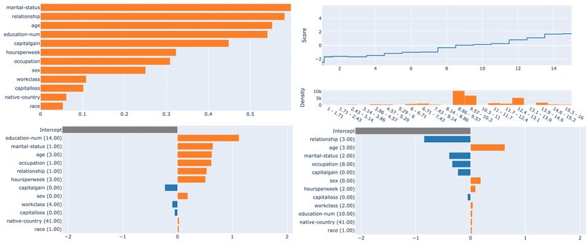
2       F. Bodria, F. Giannotti, R. Guidotti, F. Naretto, D. Pedreschi

of the explainers. Furthermore, we include a quantitative numerical comparison of some of the
explanation methods aimed at testing their faithfulness, stability, robustness, and running time.
    The rest of the paper is organized as follows. Section 2 summarizes existing surveys on ex-
plainability in AI and interpretability in ML and highlights the differences between this work and
previous ones. Then, Section 3 presents the proposed categorization based on the type of expla-
nation returned by the explainer and on the data format under analysis. Sections 4, 5, 6 present
the details of the most recent and widely adopted explanation methods together with a qualitative
and quantitative comparison. Finally, Section 8 summarizes the crucial aspects that emerged from
the analysis of the state of the art and future research directions.

2   Related Works

The widespread need for XAI in the last years caused an explosion of interest in the design of
explanation methods [52]. For instance, in the books [90,105] are presented in details the most well-
known methodologies to make general machine learning models interpretable [90] and to explain
the outcomes of deep neural networks [105].
    In [59], the classification is based on four categories of problems, and the explanation methods
are classified according to the problem they are able to solve. The first distinction is between ex-
planation by design (also named intrinsic interpretability and black-box explanation (also named
post-hoc interpretability [3,92,26]). The second distinction in [59], further classify the black-box ex-
planation problem into model explanation, outcome explanation and black-box inspection. Model
explanation, achieved by global explainers [36], aims at explaining the whole logic of a model.
Outcome explanation, achieved by local explainers [102,84], understand the reasons for a specific
outcome. Finally, the aim of black-box inspection, is to retrieve a visual representation for un-
derstanding how the black-box works. Another crucial distinction highlighted in [86,59,3,44,26] is
between model-specific and model-agnostic explanation methods. This classification depends on
whether the technique adopted to explain can work only on a specific black-box model or can be
adopted on any black-box.
    In [50], the focus is to propose a unified taxonomy to classify the existing literature. The follow-
ing key terms are defined: explanation, interpretability and explainability. An explanation answers
a “why question” justifying an event. Interpretability consists of describing the internals of a sys-
tem in a way that is understandable to humans. A system is called interpretable if it produces
descriptions that are simple enough for a person to understand using a vocabulary that is meaning-
ful to the user. An alternative, but similar, classification of definitions is presented in [13], with a
specific taxonomy for explainers of deep learning models. The leading concept of the classification
is Responsible Artificial Intelligence, i.e., a methodology for the large-scale implementation of AI
methods in real organizations with fairness, model explainability, and accountability at its core.
Similarly to [59], in [13] the term interpretability (or transparency) is used to refer to a passive
characteristic of a model that makes sense for a human observer. On the other hand, explainability
is an active characteristic of a model, denoting any action taken with the intent of clarifying or de-
tailing its internal functions. Further taxonomies and definitions are presented in [92,26]. Another
branch of the literature review is focusing on the quantitative and qualitative evaluation of expla-
nation methods [105,26]. Finally, we highlight that the literature reviews related to explainability
are focused not just on ML and AI but also on social studies [87,24], recommendation systems [131],
model-agents[10], and domain-specific applications such as health and medicine [117].
    In this survey we decided to rewrite the taxonomy proposed in [59] but from a data type
perspective. In light of the works mentioned above, we believe that an updated systematic cate-
gorization of explanation methods based on the type of explanation returned and comparing the
explanations is still missing in the literature.

3   Explanation-Based Categorization of Explainers and Evaluation
    Measures

This paper aims to categorize explanation methods concerning the type of explanation returned
and present the most widely adopted quantitative evaluation measures to validate explanations
under different aspects and benchmark the explainers adopting these measures. The objective is to
provide to the reader a guide to map a black-box model to a set of compatible explanation methods.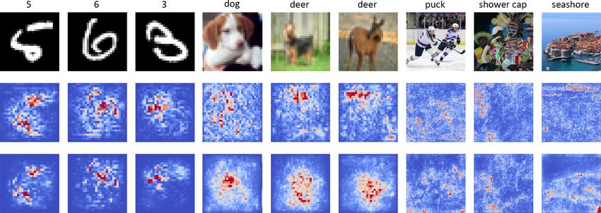
Benchmarking and Survey of Explanation Methods for Black Box Models 3
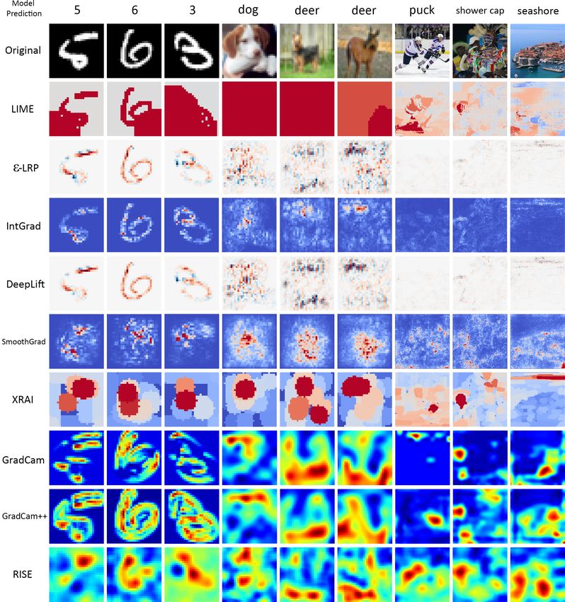
Table 1: Examples of explanations divided for different data type and explanation
TABULAR IMAGE TEXT
Saliency Maps (SM)
A map which highlight the Sentence Highlighting (SH)
Rule-Based (RB)
contribution of each pixel at the A map which highlight the
A set of premises that the
prediction. contribution of each word at the
record must satisfy in order to
prediction.
meet the rule’s consequence.
r = Education ≤ College
→ ≤ 50k
Concept Attribution (CA) Attention Based (AB)
Feature Importance (FI)
Compute attribution to a target This type of explanation gives a
A vector containing a value for
“concept” given by the user. For matrix of scores which reveal
each feature. Each value
example, how sensitive is the how the word in the sentence
indicates the importance of the
output (a prediction of zebra) to are related to each other.
feature for the classification.
a concept (the presence of
stripes)?
Prototypes (PR)
The user is provided with a series of examples that characterize a class of the black box
p = Age ∈ [35, 60], Education → p = “... not bad ...” →
p=
∈ [College, Master] →“≥ 50k” “cat” “positive”
Counterfactuals (CF)
The user is provided with a series of examples similar to the input query but with different class
prediction
q = Education ≤ College →
“≤ 50k” q= →“3” c = →“8”
c = Education ≥ Master →
“≥ 50k”
q=
The movie is not that bad →“positive”
c=
The movie is that bad →“negative”
Furthermore, we systematically present a qualitative comparison of the explanations that also help
understand how to read these explanations returned by the different methods7 .
3.1 Categorization of Type of Explanations
In this survey, we present explanations and explanation methods acting on the three principal data
types recognized in the literature: tabular data, images and text [59]. In particular, for every of
these data types, we have distinguished different types of explanations illustrated in Table 1. A
Table appearing at the beginning of each subsequent Section summarizes the explanation methods
by grouping them accordingly to the classification illustrated in Table 1. Besides, in every section
we present the meaning of each type of explanation. The acronyms reported in capital letters in
Table 1, in this section and in the following are used in the remainder of the work to quickly
categorize the various explanations and explanation methods. We highlight that the nature of this
work is tied to test the available libraries and toolkits for XAI. Therefore, the presentation of the
existing methods is focused on the most recent works (specifically from 2018 to the date of writing)
and to those papers providing a usable implementation that is nowadays widely adopted.
7
All the experiments in the next sections are performed on a server with GPU: 1xTesla K80 , compute 3.7,
having 2496 CUDA cores , 12GB GDDR5 VRAM, CPU: 1xsingle core hyper threaded Xeon Processors
@2.3Ghz i.e (1 core, 2 threads) with 16 GB of RAM, or on a server: CPU: 16x Intel(R) Xeon(R)
Gold 5120 CPU @ 2.20GHz (64 bits), 63 gb RAM. The code for reproducing the results is available
https://github.com/kdd-lab/XAI-Survey.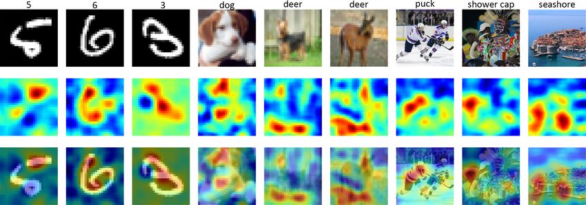
4         F. Bodria, F. Giannotti, R. Guidotti, F. Naretto, D. Pedreschi

                Fig. 1: Existing taxonomy for the classification of explanation methods.

3.2     Existing XAI Taxonomy for Explanation Methods
In this section, we synthetically recall the existing taxonomy and classification of XAI meth-
ods present in the literature [59,3,50,13,105,26] to allow the reader to complete the proposed
explanation-based categorization of explanation methods. We summarize the fundamental distinc-
tions adopted to annotate the methods in Figure 1.
    The first distinction separates explainable by design methods from black-box explanation meth-
ods:
    – Explainable by design methods are INtrinsically (IN) explainable methods that returns a
      decision, and the reasons for the decision are directly accessible because the model is transpar-
      ent.
    – Black-box explanation are Post-Hoc (PH) explanation methods that provides explanations
      for a non interpretable model that takes decisions.
      The second differentiation distinguishes post-hoc explanation methods in global and local:
    – Global (G) explanation methods aim at explaining the overall logic of a black-box model.
      Therefore the explanation returned is a global, complete explanation valid for any instance;
    – Local (L) explainers aim at explaining the reasons for the decision of a black-box model for
      a specific instance.
      The third distinction categorizes the methods into model-agnostic and model-specific:
    – Model-Agnostic (A) explanation methods can be used to interpret any type of black-box
      model;
    – Model-Specific (S) explanation methods can be used to interpret only a specific type of
      black-box model.
   To provide to the reader a self-contained review of XAI methods, we complete this section
by rephrasing succinctly and unambiguously the definitions of explanation, interpretability, trans-
parency, and complexity:
    – Explanation [13,59] is an interface between humans and an AI decision-maker that is both
      comprehensible to humans and an accurate proxy of the AI. Consequently, explainability is the
      ability to provide a valid explanation.
    – Interpretability[59], or comprehensibility [51], is the ability to explain or provide the meaning
      in understandable terms a human. Interpretability and comprehensibility are normally tied to
      the evaluation of the model complexity.
    – Transparency [13], or equivalently understandability or intelligibility, is the capacity of a model
      of being interpretable itself. Thus, the model allows a human to understand its functioning
      without explaining its internal structure or the algorithmic means by which the model processes
      data internally.
    – Complexity [42] is the degree of effort required by a user to comprehend an explanation. The
      complexity can consider the user background or eventual time limitation necessary for the
      understanding.

3.3     Evaluation Measures
The validity and the utility of explanations methods should be evaluated in terms of goodness,
usefulness, and satisfaction of explanations. In the following, we describe a selection of established
methodologies for the evaluation of explanation methods both from the qualitative and quantitative
point of view. Moreover, depending on the kind of explainers under analysis, additional evaluation
criteria may be used. Qualitative evaluation is important to understand the actual usability of
explanations from the point of view of the end-user: they satisfy human curiosity, find meanings,
safety, social acceptance and trust. In [42] is proposed a systematization of evaluation criteria into
three major categories: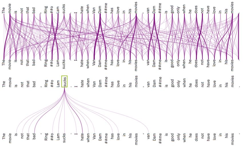
Benchmarking and Survey of Explanation Methods for Black Box Models          5

 1. Functionally-grounded metrics aim to evaluate the interpretability by exploiting some for-
    mal definitions that are used as proxies. They do not require humans for validation. The
    challenge is to define the proxy to employ, depending on the context. As an example, we can
    validate the interpretability of a model by showing the improvements w.r.t. to another model
    already proven to be interpretable by human-based experiments.
 2. Application-grounded evaluation methods require human experts able to validate the spe-
    cific task and explanation under analysis [124,114]. They are usually employed in specific
    settings. For example, if the model is an assistant in the decision making process of doctors,
    the validation is done by the doctors.
 3. Human-grounded metrics evaluate the explanations through humans who are not experts.
    The goal is to measure the overall understandability of the explanation in simplified tasks [78,73].
    This validation is most appropriate for general testing notions of the quality of an explanation.

Moreover, in [42,43] are considered several other aspects: the form of the explanation; the number
of elements the explanation contains; the compositionality of the explanation, such as the ordering
of FI values; the monotonicity between the different parts of the explanation; uncertainty and
stochasticity, which take into account how the explanation was generated, such as the presence of
random generation or sampling.
    In quantitative evaluation, the evaluation focuses on the performance of the explainer and how
close the explanation method f is to the black-box model b. Concerning quantitative evaluation
we can consider two different types of criteria:

 1. Completeness w.r.t. the black-box model. The metrics aim at evaluating how closely f
    approximates b.
 2. Completeness w.r.t. to specific task. The evaluation criteria are tailored for a particular
    task or behavior.

In the first criterion, we group the metrics that are often used in the literature [102,103,58,115].
One of the metric most used in this setting is the fidelity that aims to evaluate how good is f
at mimicking the black-box decisions. There are different specializations of fidelity, depending on
the type of explanator under analysis [58]. For example, in methods where there is a creation of a
surrogate model g to mimic b, fidelity compares the prediction of b and g on the instances Z used
to train g.
    Another measure of completeness w.r.t. b is the stability, which aims at validating how con-
sistent the explanations are for similar records. The higher the value, the better is the model
to present similar explanations for similar inputs. Stability can be evaluated by exploiting the
Lipschitz constant [8] as Lx = max kekx−xx −ex0 k    0
                                             0 k , ∀x ∈ Nx where x is the explained instance, ex the

explanation and Nx is a neighborhood of instances x0 similar to x.
    Besides the synthetic ground truth experimentation proposed in [55], a strategy to validate the
correctness of the explanation e = f (b, x) is to remove the features that the explanation method f
found important and see how the performance of b degrades. These metrics are called deletion and
insertion [97]. The intuition behind deletion is that removing the “cause” will force the black-box
to change its decision. Among the deletion methods, there is the faithfulness [8] which is tailored for
FI explainers. It aims to validate if the relevance scores indicate true importance: we expect higher
importance values for attributes that greatly influence the final prediction8 . Given a black-box b
and the feature importance e extracted from an importance-based explanator f , the faithfulness
method incrementally removes each of the attributes deemed important by f . At each removal, the
effect on the performance of b is evaluated. These values are then employed to compute the overall
correlation between feature importance and model performance. This metrics corresponds to a value
between −1 and 1: the higher the value, the better the faithfulness of the explanation. In general,
a sharp drop and a low area under the probability curve mean a good explanation. On the other
hand, the insertion metric takes a complementary approach. monotonicity is an implementation
of an insertion method: it evaluates the effect of b by incrementally adding each attribute in order
of increasing importance. In this case, we expect that the black-box performance increases by
adding more and more features, thereby resulting in monotonically increasing model performance.
Finally, other standard metrics, such as accuracy, precision and recall, are often evaluated to test
the performance of the explanation methods. The running time is also an important evaluation.

8
    An implementation of the faithfulness is available in aix360, presented in Section 7
6          F. Bodria, F. Giannotti, R. Guidotti, F. Naretto, D. Pedreschi

Table 2: Summary of methods for explaining black-boxes for tabular data. The methods are sorted
by explanation type: Features Importance (FI), Rule-Based (RB), Counterfactuals (CF), Proto-
types (PR), and Decision Tree (DT). For every method, there is a data type on which it is possible
to apply it: only on tabular (TAB) or any data (ANY). If it is an Intrinsic Model (IN) or a Post-
Hoc one (PH), a local method (L) or a global one (G), and finally if it is model agnostic (A) or
model-specific (S).
    Type         Name        Ref.      Authors        Year Data Type IN/PH G/L A/S Code
                  shap        [84]  Lundberg et al.   2007   ANY       PH   G/L A   link
                  lime       [102]   Ribeiro et al.   2016   ANY       PH    L  A   link
      FI
                   lrp        [17]     Bach et al.    2015   ANY       PH    L  A   link
                 dalex        [19]    Biecek et al.   2020   ANY       PH   L/G A   link
                  nam          [6]   Agarwal et al.   2020   TAB       PH    L   S  link
                   ciu         [9] Anjomshoae et al. 2020    TAB       PH    L  A   link
                 maple        [99]    Plumb et al.    2018   TAB      PH/IN  L  A   link
                anchor       [103]   Ribeiro et al.   2018   TAB       PH   L/G A   link
                 lore         [58]   Guidotti et al.  2018   TAB       PH    L  A   link
                slipper       [34]    Cohen et al.    1999   TAB       IN    L   S  link
                   lri       [123]    Weiss et al.    2000   TAB       IN    L   S    -
                mlrule        [39]  Domingos et al.   2008   TAB       IN   G/L  S  link
                rulefit       [48]  Friedman et al.   2008   TAB       IN   G/L  S  link
             scalable-brl    [127]    Yang et al.     2017   TAB       IN   G/L A     -
              rulematrix      [88]    Ming et al.     2018   TAB       PH   G/L A   link
      RB
                   ids        [78]  Lakkaraju et al.  2016   TAB       IN   G/L  S  link
                trepan        [36]   Craven et al.    1996   TAB       PH    G   S  link
               dectext        [22]     Boz et al.     2002   TAB       PH    G   S    -
                 msft         [31]  Chipman et al.    1998   TAB       PH    G   S    -
                  cmm         [41]  Domingos et al.   1998   TAB       PH    G   S    -
                   sta       [132]    Zhou et al.     2016   TAB       PH    G   S    -
              skoperule       [48]   Gardin et al.    2020   TAB       PH   L/G A   link
               glocalx       [107]    Setzu et al.    2019   TAB       PH   L/G A   link
              mmd-critic      [74]     Kim et al.     2016   ANY       IN    G   S  link
              protodash       [61] Gurumoorthy et al. 2019   TAB       IN    G   A  link
      PR
                   tsp       [116]     Tan et al.     2020   TAB       PH    L   S    -
                    ps        [20]     Bien et al.    2011   TAB       IN   G/L  S    -
                  cem         [40] Dhurandhar et al. 2018    ANY       PH    L   S  link
                  dice        [91]   Mothilal et al.  2020   ANY       PH    L  A   link
      CF
                  face       [100]   Poyiadzi et al.  2020   ANY       PH    L  A     -
                   cfx         [7]    Albini et al.   2020   TAB       PH    L  IN    -

4     Explanations for Tabular Data

In this Section we present a selection of approaches for explaining decision systems acting on tabular
data. In particular, we present the following types of explanations based on: Features Importance
(FI, Section 4.1), Rules (RB, Section 4.2), Prototype (PR) and Counterfactual (CF) (Section 4.3).
Table 2 summarizes and categorizes the explainers. After the presentation of the explanation
methods, we report experiments obtained from the application of them on two datasets9 : adult
and german. We trained the following ML models: Logistic Regression (LG), XGBoost (XGB), and
Catboost (CAT).

4.1    Feature Importance

Feature importance is one of the most popular types of explanation returned by local explanation
methods. The explainer assigns to each feature an importance value which represents how much
that particular feature was important for the prediction under analysis. Formally, given a record
x, an explainer f (·) models a feature importance explanation as a vector e = {e1 , e2 , . . . , em }, in
which the value ei ∈ e is the importance of the ith feature for the decision made by the black-box
model b(x). For understanding the contribution of each feature, the sign and the magnitude of
each value ei are considered. W.r.t. the sign, if ei < 0, it means that feature contributes negatively
for the outcome y; otherwise, if ei > 0, the feature contributes positively. The magnitude, instead,
9
    adult: https://archive.ics.uci.edu/ml/datasets/adult, german: https://archive.ics.uci.edu/
    ml/datasets/statlog+(german+credit+data)
Benchmarking and Survey of Explanation Methods for Black Box Models         7

Fig. 2: TOP : lime application on the same record for adult (a/b), german (c/d): a/c are the LG
model explanation and b/d the CAT model explanation. All the models correctly predicted the
output class. BOTTOM : Force plot returned by shap explaining XGB on two records of adult: (e),
labeled as class 1 (> 50K) and, (f), labeled as class 0 (≤ 50K). Only the features that contributed
more (i.e. higher shap’s values) to the classification are reported.

represents how great the contribution of the feature is to the final prediction y. In particular,
the greater the value of |ei |, the greater its contribution. Hence, when ei = 0 it means that the
ith feature is showing no contribution for the output decision. An example of a feature based
explanation is e = {age = 0.8, income = 0.0, education = −0.2}, y = deny. In this case, age is the
most important feature for the decision deny, income is not affecting the outcome and education
has a small negative contribution.
    LIME, Local Interpretable Model-agnostic Explanations [102], is a model-agnostic explanation
approach which returns explanations as features importance vectors. The main idea of lime is that
the explanation may be derived locally from records generated randomly in the neighborhood of the
instance that has to be explained. The key factor is that it samples instances both in the vicinity of
x (which have a high weight) and far away from x (low weight), exploiting πx , a proximity measure
able to capture the locality. We denote b the black-box and x the instance we want to explain.
To learn the local behavior of b, lime draws samples weighted by πx . It samples these instances
around x by drawing nonzero elements of x uniformly at random. This gives to lime a perturbed
sample of instances {z ∈ Rd } to fed to the model b and obtain b(z). They are then used to train
the explanation model g(·): a sparse linear model on the perturbed samples. The local feature
importance explanation consists of the weights of the linear model. A number of papers focus on
overcoming the limitations of lime, providing several variants of it. dlime [130] is a deterministic
version in which the neighbors are selected from the training data by an agglomerative hierarchical
clustering. ilime [45] randomly generates the synthetic neighborhood using weighted instances.
alime [108] runs the random data generation only once at “training time”. kl-lime [96] adopts
a Kullback-Leibler divergence to explain Bayesian predictive models. qlime [23] also consider
nonlinear relationships using a quadratic approximation.
    In Figure 2 are reported examples of lime explanations relative to our experimentation on
adult (top) and german (bottom)10 . We fed the same record into two black-boxes, and then
we explained it. Interestingly, for adult, lime considers a similar set of features as important
(even if with different values of importance) for the two models: on 6 features, only one differs. A
different scenario is obtained by the application of lime on german: different features are considered
necessary by the two models. However, the confidence of the prediction between the two models
is quite different: both of them predict the output label correctly, but CAT has a higher value,
suggesting that this could be the cause of differences between the two explanations.
    SHAP, SHapley Additive exPlanations [84], is a local-agnostic explanation method, which
can produce several types of models. All of them compute shap values: a unified measure of
feature importance based on the Shapley values11 , a concept from cooperative game theory. In
10
     For reproducibility reasons, we fixed the random seed.
11
     We refer the intrested reader to: https://christophm.github.io/interpretable-ml-book/shapley.
     html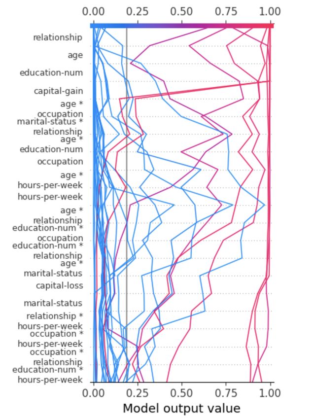
8      F. Bodria, F. Giannotti, R. Guidotti, F. Naretto, D. Pedreschi

Fig. 3: shap application on adult: a record labelled > 50K (top-left) and one as ≤ 50K(top-right).
They are obtained applying the TreeExplainer on a XGB model and then the decision plot, in which
all the input features are shown. At the bottom, the application of shap to explain the outcome
of a set of record by XGB on adult. The interaction values among the features are reported.

particular, the different explanation models proposed by shap differ in how they approximate the
computation of the shap values. All the explanation models provided by shap are     PMcalled additive
feature attribution methods and respect the following definition: g(z 0 ) = φ0 + i=1 φi zi0 , where
z 0 ≈ x as a real number, z 0 ∈ [0, 1], φi ∈ R are effects assigned to each feature, while M is the
number of simplified input features. shap has 3 properties: (i) local accuracy, meaning that g(x)
matches b(x); (ii) missingness, which allows for features xi = 0 to have no attributed impact on the
shap values; (iii) consistency, meaning that if a model changes so that the marginal contribution of
a feature value increases (or stays the same), the shap value also increases (or stays the same). The
construction of the shap values allows to employ them both locally, in which each observation gets
its own set of shap values; and globally, by exploiting collective shap values. There are 5 strategies
to compute shap’s values: KernelExplainer, LinearExplainer, TreeExplainer, GradientExplainer,
and DeepExplainer. In particular, the KernelExplainer is an agnostic method while the others are
specifically designed for different kinds of ML models.
    In our experiments with shap we applied: (i) the LinearExplainer to the LG models, (ii) the
TreeExplainer to the XGB and (iii) KernelExplainer to the CAT models. In Figures 2 we report
the application of shap on adult through force plot. The plot shows how each feature contributes
to pushing the output model value away from the base value, which is an average among the
training dataset’s output model values. The red features are pushing the output value higher while
the ones in blue are pushing it lower. For each feature is reported the actual value for the record
under analysis. Only the features with the highest shap values are shown in this plot. In the first
force plot, the features that are pushing the value higher are contributing more to the output value,
and it is possible to note it by looking at the base value (0.18) and the actual output value (0.79).
In the force plot on the right, the output value is 0.0, and it is interesting to see that only Age,
Relationship and Hours Per Week are contributing to pushing it lower. Figure 3 (left and center)
depicts the decision plots: in this case, we can see the contribution of all the input features in
decreasing order of importance. In particular, the line represents the feature importance for the
record under analysis. The line starts at its corresponding observations’ predicted value. In the
first plot, predicted as class > 50k, the feature Occupation is the most important, followed by Age
and Relationship. For the second plot, instead, Age, Relationship and Hours Per Week are the
most important feature. Besides the local explanations, shap also offers a global interpretation of
the model-driven by the local interpretations. Figure 3 (right) reports a global decision plot that
represents the feature importance of 30 records of adult. Each line represents a record, and the
predicted value determines the color of the line.
    DALEX [19] is a post-hoc, local and global agnostic explanation method. Regarding local ex-
planations, dalex contains an implementation of a variable attribution approach [104]. It consists
of a decomposition of the model’s predictions, in which each decomposition can be seen as a local
gradient and used to identify the contribution of each attribute. Moreover, dalex contains the
ceteris-paribus profiles, which allow for a What-if analysis by examining the influence of a variable
by fixing the others. Regarding the global explanations, dalex contains different exploratory tools:
model performance measures, variable importance measures, residual diagnoses, and partial depen-
dence plot. In Figure 4 are reported some local explanations obtained by the application of dalex
to an XGB model on adult. On the left are reported two explanation plots for a record classified
as class > 50k. On the top, there is a visualization based on Shapely values, which highlights as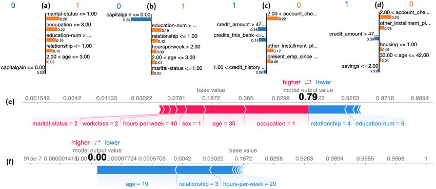
Benchmarking and Survey of Explanation Methods for Black Box Models            9

Fig. 4: Explanations of dalex for two records of adult: b(x) = 0 (≤ 50) (left), b(x) = 1 (> 50K)
(right) to explain an XGB in form of Shapely values (top), break down plots (bottom). The y-axis
is the features important, the x-axis the positive/negative contribution.

Fig. 5: TOP : Results of ebm on adult: overall global explanation (left), example of a global expla-
nation for education number (right).
BOTTOM : Local explanations of ebm on adult: left, a record classified as 1 (> 50K); right a
record classified as 0 (≤ 50).

most important the feature Age (35 years old), followed by occupation. At the bottom, there is a
Breakdown plot, in which the green bars represent positive changes in the mean predictions, while
the red ones are negative changes. The plot also shows the intercept, which is the overall mean
value for the predictions. It is interesting to see that Age and occupation are the most important
features that positively contributed to the prediction for both the plots. In contrast, Sex is posi-
tively important for Shapely values but negatively important for the Breakdown plot. On the right
part of Figure 4 we report a record classified as < 50k. In this case, there are important differences
in the feature considered most important by the two methods: for the Shapely values, Age and
Relationship are the two most important features, while in the Breakdown plot Hours Per Week
is the most important one.
    CIU, Contextual Importance and Utility [9], is a local, agnostic explanation method. ciu is
based on the idea that the context, i.e., the set of input values being tested, is a key factor in
generating faithful explanations. The authors suggest that a feature that may be important in a
context may be irrelevant in another one. ciu explains the model’s outcome based on the contextual
importance (CI), which approximates the overall importance of a feature in the current context,
and on the contextual utility (CU), which estimates how good the current feature values are for a
given output class. Technically, ciu computes the values for CI and CU by exploiting Monte Carlo
simulations. We highlight that this method does not require creating a simpler model to employ
for deriving the explanations.
    NAM, Neural Additive Models [6], is a different extension of gam. This method aims to
combine the performance of powerful models, such as deep neural networks, with the inherent
intelligibility of generalized additive models. The result is a model able to learn graphs that describe
10        F. Bodria, F. Giannotti, R. Guidotti, F. Naretto, D. Pedreschi

      x = { Education = Bachelors, Occupation
                                                        x = { Education = College, Occupation = Sales,
          = Prof-specialty, Sex = Male, Na-
                                                            Sex = Male, NativeCountry = US, Age =
          tiveCountry = Vietnam, Age = 35,
                                                            19, Workclass = 2, HoursWeek = 15, Race
          Workclass = 3, HoursWeek = 40, Race
                                                            = White, MaritialStatus = Married-civ,
          =    Asian-Pac-Islander,   MaritialStatus
                                                            Relationship = Husband, CapitalGain =
          =Married-civ, Relationship = Husband,
                                                            2880, CapitalLoss = 0 }, ≤ 50k
          CapitalGain = 0, CapitalLoss = 0}, > 50k
      ranchor = { EducationNum > Bachelors,             ranchor = {Education ≤ College,
                Occupation ≤ 3.00, HoursWeek > 20,                MaritialStatus > 1.00 } → ≤ 50k
                Relationship ≤ 1.00, 34 < Age ≤ 41 }
                → > 50k
                                                        rlore = {Education ≤ Masters, Occupation >
      rlore = { Education > 5-6th, Race > 0.86,
                                                                -0.34, HoursWeek ≤ 40, WorkClass ≤
              WorkClass ≤ 3.41, CapitalGain ≤ 20000,
                                                                3.50, CapitalGain ≤ 10000, Age ≤ 34}
              CapitalLoss ≤ 1306 } → > 50k
                                                                → ≤ 50k
                                                        clore = {Education > Masters } → > 50k
      clore = {CapitalLoss ≥ 436 } → ≤ 50k
                                                                {CapitalGain > 20000 } → > 50k
                                                                {Occupation ≤ -0.34 } → > 50k

           Fig. 6: Explanations of anchor and lore for adult to explain an XGB model.

how the prediction is computed. nam trains multiple deep neural networks in an additive fashion
such that each neural network attend to a single input feature.

4.2     Rule-based Explanation

Decision rules give the end-user an explanation about the reasons that lead to the final prediction.
The majority of explanation methods for tabular data are in this category since decision rules are
human-readable. A decision rule r, also called factual or logic rule [58], has the form p → y, in
which p is a premise, composed of a Boolean condition on feature values, while y is the consequence
                                                                                        (l) (u)
of the rule. In particular, p is a conjunction of split conditions of the form xi ∈[vi , vi ], where
                       (l) (u)
xi is a feature and vi , vi are lower and upper bound values in the domain of xi extended with
±∞. An instance x satisfies r, or r covers x, if every Boolean conditions of p evaluate to true for
x. If the instance x to explain satisfies p, the rule p → y represents then a candidate explanation
of the decision g(x) = y. Moreover, if the interpretable predictor mimics the behavior of the black-
box in the neighborhood of x, we further conclude that the rule is a candidate local explanation
of b(x) = g(x) = y. We highlight that, in the context of rules we can also find the so-called
counterfactual rules [58]. Counterfactual rules have the same structure of decision rules, with the
only difference that the consequence of the rule y is different w.r.t. b(x) = y. They are important
to explain to the end-user what should be changed to obtain a different output. An example of a
rule explanation is r = {age < 40, income < 30k, education ≤ Bachelor }, y = deny. In this case,
the record {age = 18, income = 15k, education = Highschool } satisfies the rule above. A possible
counterfactual rule, instead can be: r = {income > 40k, education ≥ Bachelor }, y = allow .
    ANCHOR [103] is a model-agnostic system that outputs rules as explanations. This approach’s
name comes from the output rules, called anchors. The idea is that, for decisions on which the
anchor holds, changes in the rest of the instance’s feature values do not change the outcome.
Formally, given a record x, r is an anchor if r(x) = b(x). To obtain the anchors, anchor perturbs
the instance x obtaining a set of synthetic records employed to extract anchors with precision
above a user-defined threshold. First, since the synthetic generation of the dataset may lead to a
massive number of samples anchor exploits a multi-armed bandit algorithm [72]. Second, since
the number of all possible anchors is exponential anchor uses a bottom-up approach and a beam
search. Figure 6 reports some rules obtained by applying anchor to a XGB model on adult. The
first rule has a high precision (0.96%) but a very low coverage (0.01%). It is interesting to note that
the first rule contains Relationship and Education Num, which are the features highlighted by most
of the explanation models proposed so far. In particular, in this case, for having a classification
> 50k, the Relationship should be husband and the Education Num at least bachelor degree.
Education Num can also be found in the second rule, in which case has to be less or equal to
College, followed by the Maritial Status, which can be anything other than married with a civilian.
This rule has an even better precision (0.97%) and suitable coverage (0.37%).
Benchmarking and Survey of Explanation Methods for Black Box Models 11
r = {Age > 34, HoursPerWeek > 20, r = { Age ≤ 19, WorkClass ≤ 4.5,
Education > 12.5, Occupation ≤ 3.5, HoursPerWeek ≤ 30, Education ≤ 13.5,
Relationship ≤ 2.5, CapitalGain ≤ 20000, Education > 3.5, MaritialStatus > 2.5,
CapitalLoss ≤ 223} → 1 Relationship > 2.5, CapitalLoss ≤ 1306 } → 0
{ Prec = 0.79 %, Rec = 0.15 %, Cov = 1 } { Prec = 0.99 %, Rec = 0.19 %, Cov = 1 }
Fig. 7: skoperule global explanations of XGB on adult. On the left, a rule for class > 50k, on
the right for class < 50k.
LORE, LOcal Rule-based Explainer [58], is a local agnostic method that provides faithful
explanations in the form of rules and counterfactual rules. lore is tailored explicitly for tabular
data. It exploits a genetic algorithm for creating the neighborhood of the record to explain. Such
a neighborhood produces a more faithful and dense representation of the vicinity of x w.r.t. lime.
Given a black-box b and an instance x, with b(x) = y, lore first generates a synthetic set Z
of neighbors through a genetic algorithm. Then, it trains a decision tree classifier g on this set
labeled with the black-box outcome b(Z). From g, it retrieves an explanation that consists of two
components: (i) a factual decision rule, that corresponds to the path on the decision tree followed
by the instance x to reach the decision y, and (ii) a set of counterfactual rules, which have a different
classification w.r.t. y. This counterfactual rules set shows the conditions that can be varied on x
in order to change the output decision. In Figure 6 we report the factual and counterfactual rules
of lore for the explanation of the same records showed for anchor. It is interesting to note that,
differently from anchor and the others models proposed above, lore explanations focuses more
on the Education Num, Occupation, Capital Gain and Capital Loss, while the features about the
relationship are not present.
RuleMatrix [88] is a post-hoc agnostic explanator tailored for the visualization of the rules
extracted. First, given a training dataset and a black-box model, rulematrix executes a rule
induction step, in which a rule list is extracted by sampling the input data and their predicted
label by the black-box. Then, the rules extracted are filtered based on thresholds of confidence
and support. Finally, rulematrix outputs a visual representation of the rules. The user interface
allows for several analyses based on plots and metrics, such as fidelity.
One of the most popular ways for generating rules is by extracting them from a decision tree.
In particular, due to the method’s simplicity and interpretability, decision trees explain black-box
models’ overall behavior. Many works in this setting are model specific to exploit some structural
information of the black-box model under analysis.
TREPAN [36] is a model-specific global explainer tailored for neural networks. Given a neural
network b, trepan generates a decision tree g that approximates the network by maximizing the
gain ratio and the model fidelity.
DecText is a global model-specific explainer tailored for neural networks [22]. The aim of
dectext is to find the most relevant features. To achieve this goal, dectext resembles trepan,
with the difference that it considers four different splitting methods. Moreover, it also considers a
pruning strategy based on fidelity to reduce the final explanation tree’s size. In this way, dectext
can maximize the fidelity while keeping the model simple.
MSFT [31] is a specific global post-hoc explanation method that outputs decision trees starting
from random forests. It is based on the observation that, even if random forests contain hundreds
of different trees, they are quite similar, differing only for few nodes. Hence, the authors propose
dissimilarity metrics to summarize the random forest trees using a clustering method. Then, for
each cluster, an archetype is retrieved as an explanation.
CMM, Combined Multiple Model procedure [41], is a specific global post-hoc explanation
method for tree ensembles. The key point of cmm is the data enrichment. In fact, given an input
dataset X, cmm first modifies it n times. On the n variants of the dataset, it learns a black-box.
Then, random records are generated and labeled using a bagging strategy on the black-boxes. In
this way, the authors were able to increase the size of the dataset to build the final decision tree.
STA, Single Tree Approximation [132], is a specific global post-hoc explanation method tailored
for random forests, in which the decision tree, used as an explanation, is constructed by exploiting
test hypothesis to find the best splits.
SkopeRules is a post-hoc, agnostic model, both global and local 12 , based on the rulefit [48]
idea to define an ensemble method and then extract the rules from it. skope-rules employs fast
algorithms such as bagging or gradient boosting decision tress. After extracting all the possible
rules, skope-rules removes rules redundant or too similar by a similarity threshold. Differently
12
https://skope-rules.readthedocs.io/en/latest/skope_rules.html12 F. Bodria, F. Giannotti, R. Guidotti, F. Naretto, D. Pedreschi
from rulefit, the scoring method does not solve the L1 regularization. Instead, the weights are
given depending on the precision score of the rule. We can employ skoperules in two ways: (i)
as an explanation method for the input dataset, which describes, by rules, the characteristics of
the dataset; (ii) as a transparent method by outputting the rules employed for the prediction. In
Figure 7, we report the rule extracted by rulefit with highest precision and recall for each class
for adult. Similarly to the models analyzed so far, we can find Relationship and Education among
the features in the rules. In particular, for the first rule, for > 50k, the Education has to be at
least a Bachelor degree, while for the other class, it has to be at least fifth or sixth. Interestingly,
it is also mentioned the Capital Gain and Capital Loss which were considered as important by
few models, such as lore. We also tested skoperules to create a rule-based classifier obtaining
a precision of 0.68 on adult.
Moreover, with skoperules, it is possible to explain, using rules, the entire dataset without
considering the output labels; or obtain a set of rules for each output class. We tested both of
them, but we report only the case of rules for each class. In particular, we report the rule with the
highest precision and recall for each class for adult in Figure 7.
Scalable-BRL [127] is an interpretable probabilistic rule-based classifier that optimizes the
posterior probability of a Bayesian hierarchical model over the rule lists. The theoretical part of
this approach is based on [81]. The particularity of scalable-brl is that it is scalable, due to a
specific bit vector manipulation.
GLocalX [1] is a rule-based explanation method which exploits a novel approach: the local
to global paradigm. The idea is to derive a global explanation by subsuming local logical rules.
GLocalX start from an array of factual rules and following a hierarchical bottom up fashion
merges rules covering similar records and expressing the same conditions. GLocalX finds the
smallest possible set of rules that is: (i) general, meaning that the rules should apply to a large
subset of the dataset; (ii) has high accuracy. The final explanation proposed to end-user is a set of
rules. In [1] the authors validated the model in constrained settings: limited or no access to data
or local explanations. A simpler version of GLocalX is presented [107]: here, the final set of rules
is selected through a scoring system based on rules generality, coverage, and accuracy.
4.3 Prototypes
A prototype, also called archetype or artifact, is an object representing a set of similar records. It
can be (i) a record from the training dataset close to the input data x; (ii) a centroid of a cluster
to which the input x belongs to. Alternatively, (iii) even a synthetic record, generating following
some ad-hoc process. Depending on the explanation method considered, different definitions and
requirements to find a prototype are considered. Prototypes serve as examples: the user understands
the model’s reasoning by looking at records similar to his/hers.
MMD-CRITIC [74] is a “before the model” methodology, in the sense that it only analyses the
distribution of the dataset under analysis. It produces prototypes and criticisms as explanations for
a dataset using Maximum Mean Discrepancy (MMD). The first ones explain the dataset’s general
behavior, while the latter represent points that are not well explained by the prototypes. mmd-
critic selects prototypes by measuring the difference between the distribution of the instances
and the instances in the whole dataset. The set of instances nearer to the data distribution are
called prototypes, and the farthest are called criticisms. mmd-critic shows only minority data
points that differ substantially from the prototype but belong in the same category. For criticism,
mmd-critic selects criticisms from parts of the dataset underrepresented by the prototypes, with
an additional constraint to ensure the criticisms are diverse.
ProtoDash [61] is a variant of mmd-critic. It is an explainer that employs prototypical
examples and criticisms to explain the input dataset. Differently, w.r.t. mmd-critic, protodash
associates non-negative weights, which indicate the importance of each prototype. In this way, it
can reflect even some complicated structures.
Privacy-Preserving Explanations [21] is a local post-hoc agnostic explanability method
which outputs prototypes and shallow trees as explanations. It is the first approach that considers
the concept of privacy in explainability by producing privacy protected explanations. To achieve a
good trade-off between privacy and comprehensibility of the explanation, the authors construct the
explainer by employing micro aggregation to preserve privacy. In this way, the authors obtained a
set of clusters, each with a representative record ci , where i is the i − th cluster. From each cluster,
a shallow decision trees is extracted to provide an exhaustive explanation while having good com-
prehensibility due to the limited depth of the trees. When a new record x arrives, a representative
record and its associated shallow tree are selected. In particular, from g the representative ci closer
to x is selected, depending on the decision of the black-box.Benchmarking and Survey of Explanation Methods for Black Box Models 13
PS, Prototype Selection (ps) [20] is an interpretable model, composed by two parts. First,
the ps seeks a set of prototypes that better represent the data under analysis. It uses a set cover
optimization problem with some constraints on the properties the prototypes should have. Each
record in the original input dataset D is then assigned to a representative prototype. Then, the
prototypes are employed to learn a nearest neighbor rule classifier.
TSP, Tree Space Prototype [116], is a local, post-hoc and model-specific approach, tailored for
explaining random forests and gradient boosted trees. The goal is to find prototypes in the tree
space of the tree ensemble b. Given a notion of proximity between trees, with variants depending
on the kind of ensemble, tsp is able to extract prototypes for each class. Different variants are
proposed for allowing for the selection of a different number of prototypes for each class.
4.4 Counterfactuals
Counterfactuals describe a dependency on the external facts that led to a particular decision
made by the black-box model. It focuses on the differences to obtain the opposite prediction
w.r.t. b(x) = y. Counterfactuals are often addressed as the prototypes’ opposite. In [122] is for-
malized the general form a counterfactual explanation should have: b(x) = y was returned because
variables of x has values x1 , x2 , ..., xn . Instead, if x had values x11 , x12 , ..., x1n and all the other vari-
ables has remained constant, b(x) = ¬y would have been returned, where x is the record x with the
suggested changes. An ideal counterfactual should alter the values of the variables as little as possi-
ble to find the closest setting under which y is returned instead of ¬y. Regarding the counterfactual
explainers, we can divide them into three categories: exogenous, which generates the counterfactu-
als synthetically; endogenous, in which the counterfactuals are drawn from a reference population,
and hence they can produce more realistic instances w.r.t. the exogenous ones; or instance-based,
which exploits a distance function to detect the decision boundary of the black-box. There are
several desiderata in this context: efficiency, robustness, diversity, actionability, and plausibility,
among others [122,71,69]. To better understand the complex context and the many available pos-
sibilities, we refer the interested reader to [15,120,25]. In [25] is presented a study that evaluates
the understandability of factual and counterfactual explanations. The authors analyzed the mental
model theory, which stated that people construct models that simulate the assertions described.
They conducted experiments on a group of people highlighting that people prefer reasoning using
mental models and find it challenging to consider probability, calculus, and logic. There are many
works in this area of research; hence, we briefly present only the most representative methods in
this category.
MAPLE [99] is a post-hoc local agnostic explanation method that can also be used as a
transparent model due to its internal structure. It combines random forests with feature selection
methods to return feature importance based explanations. maple is based on two methods: SILO
and DStump. SILO is employed for obtaining a local training distribution, based on the random
forest leaves’. DStump, instead, ranks the features by importance. maple considers the best k
features from DStump to solve a weighted linear regression problem. In this case, the explanation
is the coefficient of the local linear model, i.e., the estimated local effect of each feature.
CEM, Contrastive Explanations Method [40], is a local, post-hoc and model-specific expla-
nation method, tailored for neural networks which outputs contrastive explanations. cem has two
components: Pertinent Positives (PP), which can be seen as prototypes, and are the minimal and
sufficient factors that have to be present to obtain the output y; and Pertinent Negatives (PN),
which are counterfactuals factors, that should be minimally and necessarily absent. cem is formu-
lated as an optimization problem over the perturbation variable δ. In particular, given x to explain,
cem considers x1 = x + δ, where δ is a perturbation applied to x. During the process, there are
two values of δ to minimize: δ p for the pertinent positives, and δ n for the pertinent negatives. cem
solves the optimization problem with a variant that employs an autoencoder to evaluate the close-
ness of x1 to the data manifold. ceml [14] is also a Python toolbox for generating counterfactual
explanations, suitable for ML models designed in Tensorflow, Keras, and PyTorch.
DICE, Diverse Counterfactual Explanations [91] is a local, post-hoc and agnostic method
which solves an optimization problem with several constraints to ensure feasibility and diversity
when returning counterfactuals. Feasibility is critical in the context of counterfactual since it allows
avoiding examples that are unfeasible. As an example, consider the case of a classifier that deter-
mines whether to grant loans. If the classifier denies the loan to an applicant with a low salary,
the cause may be low income. However, a counterfactual such as “You have to double your salary”
may be unfeasible, and hence it is not a satisfactory explanation. The feasibility is achieved by
imposing some constraints on the optimization problem: the proximity constraint, from [122], the14 F. Bodria, F. Giannotti, R. Guidotti, F. Naretto, D. Pedreschi
sparsity constraint, and then user-defined constraints. Besides feasibility, another essential factor
is diversity, which provides different ways of changing the outcome class.
FACE, Feasible and Actionable Counterfactual Explanations [100] is a local, post-hoc agnostic
explanation method that focuses on returning “achievable” counterfactuals. Indeed, face uncovers
“feasible paths” for generating counterfactual. These feasible paths are the shortest path distances
defined via density-weighted metrics. It can extract counterfactuals that are coherent with the
input data distribution. face generates a graph over the data points, and the user can select
the prediction, the density, also the weights, and a conditions function. face updates the graph
accordingly to these constraints and applies the shortest path algorithm to find all the data points
that satisfy the requirements.
CFX [7] is a local, post-hoc, and model-specific method that generates counterfactuals expla-
nations for Bayesian Network Classifiers. The explanations are built from relations of influence
between variables, indicating the reasons for the classification. In particular, this method’s main
achievement is that it can find pivotal factors for the classification task: these factors, if removed,
would give rise to a different classification.
4.5 Transparent methods
In this section we present some transparent methods, tailored for tabular data. In particular, we
first present some models which output feature importance, then methods which outputs rules.
EBM, Explainable Boosting Machine [93] is an interpretable ML algorithm. Technically, ebm
is a variant of a Generalized Additive Model (gam) [64], i.e., a generalized linear model that
incorporates nonlinear forms of the predictors. For each feature, ebm uses a boosting procedure to
train the generalized linear model: it cycles over the features, in a round-robin fashion, to train one
feature function at a time and mitigate the effects of co-linearity. In this way, the model learns the
best set of feature functions, which can be exploited to understand how each feature contributes
to the final prediction. ebm is implemented by the interpretml Python Library13 . We trained
an ebm on adult. In Figure 5 we show a global explanation reporting the importance for each
feature used by ebm. We observe that Maritial Status is the most important feature, followed
by Relationship and Age. In Figure 5 we show an inspection of the feature Education Number
illustrating how the prediction score changes depending on the value of the feature. In Figure 5,
are also reported two examples of local explanations for ebm. For the first record, predicted as
> 50k, the most important feature is Education Num, which is Master for this record. For the
second record, predicted as < 50k, the most important feature is Relationship. This feature is
important for both records: in the first (husband) is pushing the value higher, while in the second
(own-child) lower.
TED [65] is an intrinsically transparent approach that requires in input a training dataset in
which its explanation correlates each record. Explanations can be of any type, such as rules or
feature importance. For the training phase, the framework allows using any ML model capable
of dealing with multilabel classification. In this way, the model can classify the record in input
and correlate it with its explanation. A possible limitation of this approach is the creation of the
explanations to feed during the training phase. ted is implemented in aix360.
SLIPPER [34] is a transparent rule learner based on a modified version of Adaboost. It outputs
compact and comprehensible rules by imposing constraints on the rule builder.
LRI [123] is a transparent rule learner that achieves good performance while giving inter-
pretable rules as explanations. In lri, each class of the training is represented by a set of rules,
without ordering. The rules are obtained by an induction method that weights the cumulative error
adaptively without pruning. When a new record is considered, all the available rules are tested
on it. The output class is the one that has the most satisfying set of rules for the record under
analysis.
MlRules [39] is a transparent rule induction algorithm solving classification tasks through
probability estimation. Rule induction is done with boosting strategies, but a maximum likelihood
estimation is applied for rule generation.
RuleFit [48] is a transparent rule learner that exploits an ensemble of trees. As a first step,
it creates an ensemble model by using gradient boosting. The rules are then extracted from the
ensemble: each path in each tree is a rule. After the rules’ extraction, they are weighted according
to an optimization problem based on L1 regularization.
IDS, Interpretable Decision Sets [78], is a transparent and highly accurate model based on
decision sets. Decision sets are sets of independent, short, accurate, and non-overlapping if-then
rules. Hence, they can be applied independently.
13
https://github.com/interpretml/interpretYou can also read