OVERVIEW OF TIME SYNCHRONIZATION FOR IOT DEPLOYMENTS: CLOCK DISCIPLINE ALGORITHMS AND PROTOCOLS
←
→
Page content transcription
If your browser does not render page correctly, please read the page content below
sensors
Review
Overview of Time Synchronization for IoT
Deployments: Clock Discipline Algorithms
and Protocols
Hüseyin Yiğitler * , Behnam Badihi and Riku Jäntti
 Department of Communications and Networking, Aalto University, 02150 Espoo, Finland;
 behnam.badihi@aalto.fi (B.B.); riku.jantti@aalto.fi (R.J.)
 * Correspondence: huseyin.yigitler@aalto.fi

 Received: 31 August 2020; Accepted: 10 October 2020; Published: 20 October 2020

 Abstract: Internet of Things (IoT) is expected to change the everyday life of its users by enabling data
 exchanges among pervasive things through the Internet. Such a broad aim, however, puts prohibitive
 constraints on applications demanding time-synchronized operation for the chronological ordering
 of information or synchronous execution of some tasks, since in general the networks are formed
 by entities of widely varying resources. On one hand, the existing contemporary solutions for time
 synchronization, such as Network Time Protocol, do not easily tailor to resource-constrained devices,
 and on the other, the available solutions for constrained systems do not extend well to heterogeneous
 deployments. In this article, the time synchronization problems for IoT deployments for applications
 requiring a coherent notion of time are studied. Detailed derivations of the clock model and various
 clock relation models are provided. The clock synchronization methods are also presented for
 different models, and their expected performance are derived and illustrated. A survey of time
 synchronization protocols is provided to aid the IoT practitioners to select appropriate components
 for a deployment. The clock discipline algorithms are presented in a tutorial format, while the time
 synchronization methods are summarized as a survey. Therefore, this paper is a holistic overview of
 the available time synchronization methods for IoT deployments.

 Keywords: internet of things; capillary networks; wireless sensor networks; clock synchronization;
 clock discipline algorithms; time synchronization protocols

1. Introduction
      Recent advances in embedded intelligence, connectivity, and interaction technologies have
allowed integrating pervasive objects from our daily life into communication networks to interact with
each other over the Internet for enabling novel applications and services. This emerging communication
and computing paradigm is often referred to as Internet of Things (IoT), and it utilizes the Internet as
both communication and virtualization platform to link the physical world to the information (virtual)
world [1]. The broad interconnection possibilities supported by the IoT brings forth interoperability
problems between different objects with heterogeneous capabilities [2]. In a typical IoT deployment,
three different networks are taking part as shown in Figure 1. A node of a wide area network (WAN),
e.g., user entity of a cellular network, is connected to a node of a local area network (LAN) over a
network interface controller (NIC), and this node is connected to a personnel area network (PAN)
of a low-power and short-range wireless communication technology (Such an extension of a WAN
network toward local and personal area networks by using a WAN node as a backhaul connection
entity is also known as a capillary network [3]). Some of these objects may possess a large amount of
computational and communication resources, some may be energy constraint wireless sensor nodes,

Sensors 2020, 20, 5928; doi:10.3390/s20205928                                 www.mdpi.com/journal/sensors
Sensors 2020, 20, 5928 2 of 59
and some may be passive simple devices such as RFID tags. Although these components can be, in
principle, interconnected using contemporary Internet technologies, not all objects can accommodate
the resources required by these solutions. One approach is to use translation entities between these
devices and an interrogator to connect to the Internet, e.g., a gateway [4]. However, this approach
introduces processing and translation overhead, which alters the yield of applications requiring tight
interaction with the physical world. In this article, such applications are considered and wireless
sensor network entities are evaluated as objects interacting with the physical world.
Sensor / Short Sensor /
CPU 1 Actuator Range CPU Actuator
Radio
NIC 2 CPU 2 Short
NIC 1 CPU 3 Range Short Sensor /
Radio Range CPU Actuator
Radio
CPU 1 NIC 1
Short
Sensor / Range Sensor /
NIC 1 CPU Actuator CPU Actuator
Radio
Figure 1. An Internet of Things deployment utilizing a (Wireless) Sensor Network to interact with
the physical world. A Wide Area Network (WAN) node on the left is connected to the Internet over
a Network Interface Controller (NIC), and connected to the Local Area Network (LAN) at the center
using another NIC. One of the LAN nodes is connected to the Personal Area Network (PAN) on the
right, which realizes the Sensor Network. Each processor in the system has its own notion of time due
to different clock implementations. The network entities acting as gateways are explicitly shown.
Wireless sensor networks (WSNs) [5] are one of the enabling technologies of IoT. They transmit
acquired digital data from the physical world to the Internet or conversely receive data from the
Internet that describe actions to make some changes to the surroundings in order to reach a common
goal without human intervention [6]. This is achieved by seamlessly conveying the information content
by performing various translations between the involved communication and processing entities.
In this regard, applications requiring chronological information ordering or synchronous execution
for data fusion, or low-power networking and time-division transmission scheduling [7,8], require a
coherent notion of time, which must be shared among all the objects taking part in both processing and
communication.
The notion of the time of a clock is different than the universal time due to several factors as
discussed by Allan [9]. The impact of these errors is mitigated by:
(i) transmitting a time report of a reference clock using a messaging protocol;
(ii) mitigating non-determinism in message delivery and time measurements using a Clock
Discipline Algorithm (CDA), and;
(iii) adjusting the clocks.
For a typical IoT deployment, there are three different networks that have different notions of
time as shown in Figure 1. For WANs and LANs, the time synchronization problem has well-known
solutions such as the Network Time Protocol (NTP) [10,11] (or its tailored version the Simple Network
Time Protocol [12]), and Precision Time Protocol (PTP) [13]. For example, the WAN node (and also the
LAN nodes) may synchronize to the Internet time, e.g., using the NTP. However, the computation and
energy requirements of these solutions cannot be fulfilled by objects with constrained computational
and energy resources, and such objects call for simpler methods. The existing time synchronizationSensors 2020, 20, 5928 3 of 59
solutions for WSNs are designed for constrained devices (e.g., the PAN network in Figure 1), but their
performance is tailored for a specific application scenario. For the deployment in Figure 1, the global
notion of time in WAN and LAN nodes must still be disseminated to the PAN nodes through the radio
attached to CPU3, and there are no readily available solutions to fulfill accuracy requirement of all
application scenarios. Therefore, IoT practitioners are required to select a suitable time synchronization
solution considering the application scenario and the capabilities of the network entities to achieve the
required level of performance.
In this work, we present a comprehensive survey of time synchronization methods for IoT
deployments in the following organization. In Section 2, some motivating example applications
requiring a coherent notion of time are given, and available survey works are presented.
Thereafter, the individual components of time synchronization are discussed starting from clock
models in Section 3. The solutions of the clock synchronization problem, known as CDA, are presented
in Section 4. In Section 5, several aspects of time synchronization messaging are elaborated on, and two
example empirical time data are used in Section 6 to demonstrate the impact of time error sources.
Finally, conclusions are drawn in Section 7.
2. Background
In this section, we first introduce a general IoT platform, and then summarize several applications
that require a coherent notion of time. Thereafter, we review available time synchronization survey works.
2.1. IoT Platform
IoT is on the verge of changing the traditional concept of connectivity for everyone to connectivity
for everything anytime and anywhere [14]. It is a radically large and highly dynamic distributed
system with a massive number of entities producing and consuming information [15] to form a
common operational picture (COP) for different (novel) applications and services [6] as shown in Figure 2.
The objects in IoT are by no means limited to the entities that are directly connected to the Internet.
On the contrary, any uniquely identifiable physical entity, which may be connected to the Internet over
a gateway (interrogator) [16], is allowed. Therefore, IoT realizes ubiquitous computing and networking
by making the benefits of the technology inseparable part of the daily living environment [17], which is
expected to unprecedentedly alter the behavior of its users [18].
❆♣♣❧✐❝❛t✐♦♥s
☎✆✝s✐❝❛❧
✫ ❈❖P ■✁✂❡✄✁❡✂ ✭●✞✮
❙ r✈✐❝ s ❲♦r❧❞
Figure 2. Internet of Things concept using the Internet as a link between (physical) objects, and novel
application and services using a common operational picture (COP).
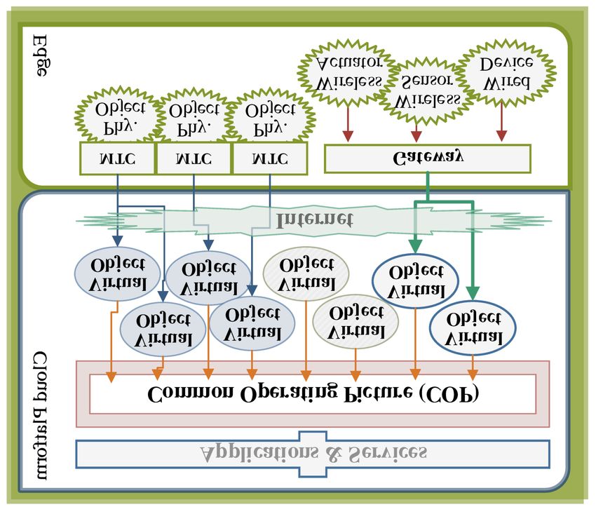
The information content of the data generated by an IoT network is used by applications and
services through the COP. Semantically, the COP does not discriminate between real objects and virtual
(information) objects, and it is natural to virtualize all the information sources and sinks as shown in
Figure 3. These entities are called virtual objects, and they may proxy physical things or they may be
linked to a software component. In either case, they represent a unit of information in the COP. Such an
information-based abstraction, in return, requires a consensus in ordering the data with respect to a
specific argument, e.g., time or frequency. For most of the physical information sources, the acquired
data is naturally ordered in time so that the information content assigned to different virtual objects
must be ordered with respect to their chronology. In particular, this is important in the following
aspects [19]:
(i) Querying the universal time at which a specific event happened and observed by an object.Sensors 2020, 20, 5928 4 of 59
(ii) Measuring the time difference between two events that are observed by different objects.
(iii) Relatively ordering the events that are observed by different objects.
Figure 3. An Internet of Things platform with physical objects deployed at the edge. Some objects
are connected to the Internet using machine-type communication (MTC) technologies whereas some
are connected over a gateway. In either case, they are represented as virtual objects in the common
operation picture, which is used by application and services.
Therefore, all the physical information sources must have a common notion of time to fuse all the
virtual objects into the COP.
2.2. Motivation
In order to build virtual objects using implicit measurements of some phenomenon, the output of
different sensors is usually fused. The acquired data from different sources are combined and correlated
to obtain additional insight, which is usually not evident in the original data [20]. The cross-correlation
of data from different sources must be calculated using the acquired samples, which requires a shared
notion of time. Therefore, implicit information sources might rely on a common notion of time among
the physical objects.
The distributed nature of WSNs allows acquiring samples from a spatio-temporal field, e.g., for
structural health monitoring [21]. These applications require collecting synchronous samples from all
the sensors to estimate the spatial parameters of interest [22]. Therefore, the synchronous execution of
certain periodic tasks, e.g., sampling, requires a coherent notion of time within the network.
Some local deployments of WSNs require a guarantee to complete a task within a certain time limit,
e.g., for industrial automation [23], recently referred to as industrial wireless sensor networks [24].
Low-jitter applications require estimation and compensation of various time uncertainty sources,
including the ones originating from oscillators and the communication entities. For these use cases,
the time-synchronized operation must be provided by the underlying networking technology, as it is
for WirelessHART or ISA100.11a standards [25]. Both of these protocols form their network using the
Time Synchronized Mesh Protocol [26], which can only be realized with tightly synchronized nodes.
These systems have recently led to the development of Time Synchronized Channel Hopping (TSCH)
networks [27], which are built upon the IEEE 802.15.4e standard [28], and have IPv6 support based
on several IETF standards [29]. For these networks, the time synchronization also enables variousSensors 2020, 20, 5928 5 of 59
techniques to improve reliability in terms of packet delivery ratio. Furthermore, the nodes are allowed
to turn-off their power-hungry components when they are not needed, which significantly decreases
power consumption. Thus, time-critical, reliable, and low-power networking solutions require tight
time-synchronization.
The advances in Mobile Adhoc Networks (MANET)s have enabled Vehicular Adhoc Networks
(VANET)s [30], which aim at realizing Intelligent Transportation Systems by supporting both
safety-related applications to reduce the probability of traffic accidents, and non-safety applications to
improve passenger comfort and accommodate commercial platforms. These networks are characterized
by their intermittent connectivity and high network node speed, and the success of just mentioned
applications depends on the accuracy of the notion of time of each vehicle [31]. In general, VANETs
can acquire precise global time from satellite-based navigation systems [32], but this may fail when
the vehicles are out of the satellite system coverage. In these cases, a global notion of time can be
disseminated in the network using the time synchronization methods for the IEEE 802.11 [33] since
the network operation is mainly based on the IEEE 802.11p [34]. Therefore, a successful realization of
intelligent transportation systems depends on the accurate notion of time within VANETs.
The management and distribution of an electricity grid using communication and pervasive
computing technologies have recently gained momentum to support distributed renewable energy
sources, which is often referred to as Smart Grid [35]. A wide-area monitoring system, fault detection,
protection functions, substation monitoring, and fault recording all require a network-wide shared
notion of time [36]. Therefore, Smart Grid IoT deployments depend on an accurate and coherent notion
of time within their network.
With the advent of the IoT in the industrial domain, which is also known as industrial IoT
(IIoT), the deployments supporting time-aware and precise timestamped operations have gained
much interest. These distributed systems are implemented using low-cost devices with the ability
to sense and monitor the physical phenomenon, and they have been deployed in the food chain
industry, industrial automation and agriculture. Most notably, these applications require low-latency
communication, precise data processing, and trusted services [37], which can only be achieved
by network-wide, accurate, and robust time-synchronization. In the remaining part of the article,
we elaborate on several aspects of time synchronization that can be used also in IIoT applications.
2.3. Related Works
The time synchronization in WSNs is one of the widely studied problems, and several survey
works exist. A summary of the available surveys is given in Table 1. The surveys [19,38–40] aim at
aiding practitioners to select or develop time synchronization protocols, and their scope is mainly
restricted to messaging schemes. In particular, a comprehensive survey by Sundararaman et al. [19]
aims at showing the link between time synchronization for WSNs, and distributed systems and wired
networks. Similarly, the works [41,42] provide classification methodologies for the available protocols.
The time synchronization problem in the signal processing perspective is studied in the survey by
Wu et al. [7], where the main scope is on exponentially distributed delivery delays. Network-wide
synchronicity and coupled-clock’s based synchronization solutions are studied in the surveys by
Simeone et al. [43], and Bojic and Nymoen [44]. The book by Serpedin and Chaudhari [45] is a
complete reference for estimation methods, and time synchronization protocols presented until 2009. It
can be concluded from the summary provided in the table that the scope of the available survey works
are constraint to certain topics of the general time synchronization problem. However, IoT networks
require one to take into account the transition of the notion of time among different networks,
which require designing different methodologies for different applications. Therefore, there is a need
for an overview survey, which is not restricted to a particular problem but presents each component
and associated solution in a bottom-up approach. In this effort, we outline individual components
taking part in the synchronization, starting from oscillators, and discuss the advantages and limitations
of available methods in the IoT deployment perspective.Sensors 2020, 20, 5928 6 of 59
Table 1. Surveys on time synchronization in WSN.
Ref. Year Content
An early survey on time synchronization methods in sensor networks. The work defines the
[38] 2004
problem, analyzes its requirements, and surveys available protocol till 2004.
A comprehensive survey on synchronization protocols in wireless sensor networks. The survey
[19] 2005 includes synchronization methods for wired networks, and provides a detailed description of
published methods till 2005. This work motivated several other articles appeared later.
[41] 2007 The earliest work that provides a set of features to classify different synchronization methods.
A survey on early distributed synchronization methods for wireless networks. The work
[43] 2008
especially summarizes the coupled-clocks based network-wide synchronization approaches.
A short survey of the most popular methods till 2010. The work aims at showing that by the
[39] 2010 time of writing, no synchronization method can provide security, scalability, topology
independence, fast convergence and energy efficiency simultaneously.
A condensed survey of WSN time synchronization in signal processing perspective.
Starting from clock relation models, several clock parameter estimators are outlined. The work
[7] 2011
especially summarizes the signal processing methods for exponentially distributed delays,
and related estimation methods.
A classification model of time synchronization methods for WSNs. The structural, technical
[42] 2015 and global objective features of available methods are identified, and a short list of protocols
are compared using the identified features.
A survey of synchronization methods for machine-to-machine type communication system.
[44] 2015 A classification taxonomy for WSN synchronization is used for motivating that biologically
inspired synchronicity is the most suitable option.
A condensed summary of time synchronization methods for wireless sensor networks
[40] 2019
realizing an IoT deployment.
In this work, we provide both a tutorial-like summary of the clock models and CDAs, and a
comprehensive survey of the time synchronization protocols. Different than the other available
surveys, the provided clock relation models are derived step by step, and various CDAs are derived
for different models. The derived clock relation model is more general than the available models,
and it shows that the time reports of software clocks are correlated in time. This correlation not
only degrades the performance of well-known estimators but also bounds the synchronization
period. The derived model is used for developing a computationally light-weight recursive clock
discipline algorithm, which is consistent and efficient. The time synchronization protocol survey
aims at providing an overview of different time synchronization components including timestamping,
messaging schemes, multi-hop approaches, and several networking practical issues and their available
solutions. A discussion on the presented components is given to clarify the advantages of the
methods. Therefore, this work aims at aiding practitioners to select appropriate clock synchronization
components in the complete IoT deployment illustrated in Figure 1.
The time synchronization is one of the widely studied problems in computer networks. In this
work, we focus primarily on the time synchronization for low-cost and low-power networks, and give
a summary of synchronization methods for LAN and WAN networks. Detailed surveys on different
time synchronous networks are tabulated in Table 2, and the reader is referred to these articles.
However, this work may still provide valuable insights on the clock models, clock discipline algorithms,
and underlying protocol primitives that affect the synchronization accuracy.Sensors 2020, 20, 5928 7 of 59
Table 2. Surveys on time synchronous networking.
Scope Ref. Year Content
Packet switched A survey on standardized protocols and technologies for synchronizing
[36] 2016
networks devices over packet-switched networks.
A survey on synchronization methods for the IEEE 802.11 (WLAN)
Wireless LAN [46] 2017
networks in infrastructure mode.
Vehicular ad-hoc A survey on available methods for, and a requirement analysis of vehicular
[31] 2018
networks ad-hoc networks.
Cellular low A survey on technologies enabling low-latency communications in radio
[47] 2018
latency networks access networks, core network, and caching.
A survey on ultra-low latency networks of IEEE time-sensitive networking
Ultra-low latency
[48] 2019 and IETF deterministic networking standards, along with ultra-low latency
networks
research studies of cellular networks.
3. Clock Models
In this section, we elaborate on the clock relation models. We first introduce the parameters
defining a software clock and then derive a model that relates the reports of one clock in terms of the
reports of another. Finally, we summarize the widely used clock relation models.
3.1. Software Clocks
A clock measures the time elapsed since an epoch. Although ideal clocks report C` (t) = t at the
universal time instant t, practical clocks can only report their time at discrete instances since they are
usually implemented as a counter driven by an oscillator [45] as shown in Figure 4. The most important
impact of such an implementation on the time reports of the clock is their deviation from the actual
time due to the imperfections of the driving oscillator. This variation is modeled as a second-order
polynomial with coefficients frequency drift ω, frequency offset γ, time-offset θ, and random variations
ε [9]. Consequently, the time deviation of a continuous clock, say C` (t), at instant t, is given by
C` (t) − t = θ` + γ` t + ω` t2 + ε ` (t), (1)
where subscripts identify the clock under consideration.
Edge-
triggered Software
counter
counter
Figure 4. An implementation of a clock.
The time deviation due to oscillator imperfections can be observed in the frequency spectrum
of a practical oscillator’s output, which is spread around localized tones rather than being non-zero
only at discrete frequencies. This phenomenon can be modeled using an ordinary differential equation
with a periodic solution, which has a phase deviation (a.k.a. time jitter) due to random perturbations.
For uncorrelated perturbation sources, the phase deviation is a Wiener process as previously shown by
Demir [49]. This result is used in previous work [50] to show that ε ` (t) can be taken as a zero-mean
Gaussian with variance σ`2 (t) and with auto-correlation function R` (t1 , t2 ) given asSensors 2020, 20, 5928 8 of 59
σ`2 (t) = (1 + γ` )2 c` t, (2a)
R` (t1 , t2 ) = c` min{t1 , t2 }, (2b)
where c` is the oscillator variance constant.
The model in Equation (1) implies also that the time error at the kth transition of the edge-triggered
counter is
T̄`
e` [k] = t − kT` = t − k, (3)
1 + γ`
where T̄` is the nominal period of the oscillator, and T` , T̄` /(1 + γ` ) is the instantaneous period.
Due to the nature of the underlying uncertainty sources discussed above, ε ` (t) is a zero mean Gaussian
process [50]. Respectively, the time error e` [k] is also a zero-mean Gaussian process with approximate
second-order statistics given as
E{e2` [k]} ≈ (1 + γ` )2 c` tk , (4a)
E{e` [k1 ]e` [k2 ]} ≈ c` min{tk1 , tk2 }, (4b)
where tk denotes the universal time when the kth sample is acquired, and E{·} denotes the
statistical expectation.
3.2. Clock Relation Model
The time deviation model in Equation (1) can be used for relating the reports of two clocks,
say the reference clock C1 (t) and the other clock C2 (t), since the universal time t is common. If there
is a message delivery delay d(t) measured in the universal time associated with the transfer of the
reference clock report C1 (t) as visualized in Figure 5, then the time report of C2 (t) when the report of
C1 (t) is received is given by
C2 (t) = α12 C1 (t) + θ12 + ε 12 (t) + (1 + γ2 )d12 (t),
1 + γ2 (5)
α12 , , θ12 , θ2 − α12 θ1 , ε 12 , ε 2 − α12 ε 1 ,
1 + γ1
where α12 is the clock skew between C1 (t) and C2 (t), and the frequency drift terms ω1 and ω2 are
ignored, following the common practice in the literature. Equation (5) is known as the clock relation
model [45], and some of its parameters are visualized in Figure 5. In the following, the clock relation
models are gradually developed.
d12(t) C2(t1)
C2(t)
C2(t0)
✂12 t0 t t1
t
C1(t0)
C1(t)
C1(t1)
Figure 5. The relation between the reports of two clocks C1 (t) and C2 (t).Sensors 2020, 20, 5928 9 of 59
3.2.1. Clocks on the Same Processor
Suppose that we are aiming to compare the time reports of clocks C1 (t) and C2 (t) that are
implemented on the same processor, that is d12 (t) = 0, and both are initialized to zero a t = 0.
The relation between the count values of the counters associated with these clocks can be written as
T̄1
m = α12 k + e [ m ],
T̄2
(6)
1
e[m] , (e [k] − e2 [m]) ,
T2 1
where m is the count value of the counter of the clock C2 (t) and k is the count value of the counter of
the clock C1 (t). The error term e[k] is also Gaussian since e1 [k] and e2 [m] are independent and Gaussian.
The second order statistics of e[k] can be derived using the statistical independence of e1 [k] and e2 [m],
which yields
1 2
E{e2 [m]} ≈ ( α c1 + c2 ) t m , (7a)
T̄22 12
1
E{e[m1 ]e[m2 ]} ≈ 2 (α212 c1 + c2 ) min{tm1 , tm2 }. (7b)
T2
The error term e[m] is zero mean if and only if the clock periods are an integer multiple of one
another, and they are phase locked so that at a universal time instant t both of the edge counters have
just incremented. This also implies that the zero mean Gaussian assumption is valid if and only if the
residual time error associated with the counter increments is negligible.
For the discrete time relation model given in Equation (6), the nominal clock periods T̄1 and T̄2 are
known constants of the oscillators, and the clock offset is zero since the clocks are implemented on the
same processor. Hence, the synchronization problem is to estimate the clock skew α12 . Let us suppose
that N time reports of both of the clocks are acquired to estimate α12 . For notational convenience,
let us define the following vectors and matrices,
k̄ = [k1 k2 − k1 · · · k N − k N −1 ] > ,
m̄ = [m1 m2 − m1 · · · m N − m N −1 ]> ,
>
ē = e[1] e[2] − e[1] · · · e[ N ] − e[ N − 1] ,
k = U k̄, m = U m̄, e = U ē,
where > denotes the matrix transpose and U is a lower triangular matrix defined as
1 0 ··· 0
1 1 ··· 0
.
U= .. .. .. ..
. . . .
1 1 ··· 1
Progressive clock relation model: Using the definitions given above, the instantaneous count values
are related to each other with
T̄
m = α12 1 k + e. (8)
T̄2Sensors 2020, 20, 5928 10 of 59
Since the time reports of clocks are monotonically increasing, this model is referred to as a progressive
time relation model, and it naturally follows from the definition of the involved quantities. For this
model, the covariance matrix of the noise term e is composed of components Q = [qij ] given as
1 2
[qij ] = (α c1 + c2 ) min{ti , t j }. (9)
T22 12
Therefore, the progressive time relation model in Equation (8) has a correlated noise term.
Incremental clock relation model: Since the lower triangular matrix U is invertible for all non-zero N,
it follows from the definition of m, k and e that
T̄1
m̄ = α12 k̄ + ē. (10)
T̄2
This time relation model operates on the incremental time reports of the clocks, and it is referred to
as the incremental clock relation model. For this model, the covariance matrix of the error term ē is a
diagonal matrix with components Q̄ = [q̄ij ] given as
1
T22
(α212 c1 + c2 )(ti − ti−1 ) i = j,
[q̄ij ] = (11)
0 i 6= j.
This diagonal matrix indicates that the incremental model in Equation (10) has independent noise
samples, enabling optimal performance for well-known estimators.
Time offset: In case the counters are reset to zero at t = 0, the clocks are related to each other
through a single parameter α12 . In order to relax this assumption, let us now suppose that the initial
count values of the counters are k0 and m0 . Then, the progressive model in Equation (8) can be
written as
T̄ T̄
m = α12 1 k + m0 − α12 1 k0 1 + e, (12)
T̄2 T̄2
where 1 is all one vector. On the other hand, for the incremental model in Equation (10), the new
time-offset term only appears in the first time report pair (m1 , k1 ), that is once the time-offset
is compensated for, the only parameter that needs to be estimated and compensated for is α12 .
Therefore, the time incremental model eliminates the need for jointly estimating the time-offset and
the clock skew, at the cost of implementing two estimators for each parameter.
3.2.2. Clocks on Different Processors
If the clock being synchronized is implemented on a different processor, there is a non-zero
time report delivery delay d12 (t). This delay depends on several message delivery implementation-
dependent factors, but all can be decomposed as
d12 (t) = D12 + δ12 (t), (13)
where D12 is deterministic and constant delays, and δ12 (t) is the random message delay at t. Thus,
a general clock relation model can be reached by including the messaging delay characteristics into
Equation (5) as
C2 (t) = α12 C1 (t) + θ12 + D12 + ε 12 (t) + δ12 (t) . (14)
| {z } | {z }
time-offset random variation
The time relation model in Equation (14) implies that the time-offset θ12 and the deterministic
delay D12 are not distinguishable and both contribute to the time-offset. Similarly, the observedSensors 2020, 20, 5928 11 of 59
random variations in the time reports of a clock compared to the reports of another follows the joint
probability distribution of ε 12 (t) and δ12 (t). In other words, a general clock relation model is given by
C2 (t) = α12 C1 (t) + τ12 + e12 (t), (15a)
τ12 , θ12 + D12 , e12 (t) , ε 12 (t) + δ12 (t), (15b)
where the time-offset τ12 and the random delay term e12 (t) have the same impact as θ12 and ε 12 (t) in
Equation (5). Therefore, the software clock relation models in Equation (6) have the same structure
even when the message delivery delay is included in the formulation.
3.2.3. Numerical Example
The time difference between clocks C1 (t) and C2 (t) grows with the reference time in accordance
with the clock relation model in Equation (14). In order to demonstrate the significance of the involved
quantities, two time series are created using the parameters in Table 3. The variation of the time reports
of a local clock C2 (tk ) with respect to the reports of a reference clock C1 (tk ) is shown in Figure 6. For the
visualized data, the reference clock reports are assumed to be transmitted every second through the
message delivery scheme with Gaussian delay of parameters given also in the table. The depicted
result shows that the variation of the difference between the time reports C2 (tk ) − C1 (tk ) with C1 (tk )
grows linearly as Equation (8) implies. Furthermore, the variance of the time difference grows as time
progresses. On the other hand, the variation of the time report increments of the node C2 (tk ) − C2 (tk−1 )
stays small and the variance does not increase as the incremental model in Equation (10) implies.
Therefore, these two models have different properties, and the clock relation model estimators for each
of the models have different characteristics as it is elaborated on in the next section.
Table 3. Time record simulation parameters.
Symbol Value Appearance Description
θ1 1 Equation (1) Time-offset of C1 in seconds
γ1 10 × 10−6 Equation (1) Frequency offset of C1
ω1 1 × 10⁻¹² Equation (1) Frequency drift of C1
c1 1 × 10⁻⁸ Equation (2a,b) Oscillator constant of C1
θ2 2 Equation (1) Time offset of C2 in seconds
γ2 −20 × 10−6 Equation (1) Frequency offset of C2
ω2 −1 × 10⁻¹⁰ Equation (1) Frequency drift of C2
c2 1 × 10⁻¹⁰ Equation (2a,b) Oscillator constant of C2
D12 1 × 10⁻³ Equation (5) Deterministic and constant message delivery delay in seconds
2 }
E{δ12 1 × 10⁻¹⁰ Equation (5) Variance of stochastic message delivery delay in seconds square
3.3. Available Clock Relation Models
Let us denote the clock relation model as
y = R( x ), (16)
where we have defined the function argument x as the reference clock reading C1 (t), and y as the local
clock reading C2 (t). The general clock relation model in Equation (6) is composed of several parameters:
oscillator-induced noise ε 12 (t) and message-delivery uncertainty δ12 (t), the initial time-offset θ12 and
deterministic message-delivery delay D12 , and the clock skew parameter α12 . The relative importance
of these parameters changes with the time record acquisition procedures, and different approximations
are possible depending on the required level of accuracy. In the following, we give a summary of the
clock relation models used in the time-synchronization literature.Sensors 2020, 20, 5928 12 of 59
1.2 C2 (tk ) − C1 (tk )
C2 (tk ) − C2 (tk−1 )
1.0
Time Difference [s]
0.8
0.6
0.4
0.2
0.0
0 5 10 15 20 25 30 35
C1 (tk ) [s] ×103
Figure 6. The time difference in seconds between the simulated local clock C2 (tk ) and the reference
time reports C1 (tk ) delivered through a Gaussian message delivery delay which are associated with
the universal time tk .
3.3.1. Offset-Only Model
The time relation model for this case is in the form
R1 ( x ) = x + τ12 , (17)
where τ12 is the time-offset, and the clock skew is assumed to be unity and constant, α12 ≡ 1. The offset
only model R1 ( x ) is an under-fitted time relation model, which has a large bias although the residual
variance is small Section 3.2 in [51].
Although, this model is not used for time-synchronization purposes under Gaussian random
variations, it is used for exponential distributed random variations by Jeske [52], by Lee et al. [53],
and by Rhee et al. [54].
3.3.2. Progressive Linear Model Only with Delivery Delay
In the pioneering work by Elson et al. [55], the impact of the oscillator-induced random time
deviation is ignored, and the time relation model is simplified to
R2 ( x ) = α12 x + τ12 + δ12 ( x ). (18)
The simplified model in Equation (18) is by far the most widely used model in the literature
(see e.g., [7,45] for a comprehensive overview). In particular, this model is used by Maróti et al. [56],
and other works (e.g., [57–59]) by assuming that the random delay δ12 ( x ) is Gaussian and its samples
in different messages are uncorrelated. The works [7,60] use the same model with an exponentially
distributed message delivery delay.
3.3.3. Incremental Linear Model Only with Delivery Delays
The progressive model in Equation (18) can be used in incremental form, which reads as
R3 ( x ) = α12 ( xk+1 − xk ) + δ12 (tk+1 ) − δ12 (tk ), (19)
where δ12 (tk+1 ) is the delivery delay term associated with xk+1 , and δ12 (tk ) is associated with xk ,
when an explicit estimate of the clock skew α12 is desired. This model is first used by Hamilton et al. [61],Sensors 2020, 20, 5928 13 of 59
and later by Yang et al. [62,63] in order to include the dynamics of the clock skew into the
synchronization problem formulation. Since this model does not contain the time offset term, it requires
a two-step clock discipline algorithm.
3.3.4. High Order Models Only with Delivery Delay
The time relation model in Equation (19) can be extended by including the temporal variation of
the clock skew in order to account for the ignored frequency drift parameter ω0 in Equation (1).
This term represents slow time variations due to the supply voltage changes, the temperature
fluctuations, and the aging of the oscillator [9]. One approach to take into account the frequency
drift is to consider a dynamical model for the clock skew α12 ,
d
α = ω12 + δα12 ( x ), (20)
dx 12
where δα12 ( x ) is the random variation of the clock skew, and the clock relation model is as in
Equation (19). This model is first proposed by Hamilton et al. [61], and it is later used by Yang et al. [62,63].
Models with an order higher than two have also been investigated by researchers. In the work by
Kim et al. [64], the authors have studied higher order autoregressive models for clock skew, where they
have also validated the model order with well-known model selection methods. The same line of
reasoning has motived Masood et al. [65] to study alternative models with both open-loop and feedback
terms. Such high order extensions cannot be easily linked to the well known physical clock parameters.
In this regard, models exceeding the second order cannot be easily described using the terminology
presented above.
3.3.5. Incremental Linear Model with Delivery Delay and Oscillator-Induced Correlation
The simplified model in Equation (18) does not take into account the correlated oscillator-induced
noise. This problem does not exist for the incremental linear model, which can be written as
R4 ( xk , xk+1 ) = α12 ( xk+1 − xk ) + e12 (tk+1 ) − e12 (tk ), (21)
where e12 (tk+1 ) is the noise term associated with xk+1 , and e12 (tk ) is associated with xk . The difference
of these two terms is uncorrelated between different increments, but the variance of the measurements
increases with the elapsed time between the reports.
The incremental linear model in Equation (21) can be generalized to cover a-periodic time report
message delivery, which is a common problem when the time reports are exchanged over a lossy
medium. For this purpose, one approach is to define the time relation model in Equation (21) as
x k +1 − x k e (t ) − e12 (tk )
1 = α12 + 12 k+1 , (22)
y k +1 − y k y k +1 − y k
where R4 ( xk , xk+1 ) = yk+1 − yk , and xk and yk are as defined above. In this case, the covariance
function of e12 (tk+1 ) − e12 (tk ) is as given in Equation (11).
The correlations in the time increments are not generally considered in the literature with the
exception of the work [50]. Such a simplification limits the performance of well-known model
estimators. As we demonstrate in the next section, taking into account the time report correlations is
important, and allows development of an efficient and consistent clock skew estimation algorithm.
However, this model does not depend on the clock offset, and requires a two-step clock discipline
algorithm development.
3.3.6. Summary
Available clock relation models presented in this section are summarized in Table 4. Every model
has some advantages and disadvantages, and each are useful under certain application requirements.Sensors 2020, 20, 5928 14 of 59
When the application does not require tight synchronization, the offset-only model can be used.
However, for other cases, a progressive first order model is usually preferred. If the application permits
a higher amount of computational resources, but limited amount of communications, higher order
models can be used. Although not widely used, the incremental model with delivery delay and
oscillator-induced correlations can be used as a direct replacement of progressive time relation model.
As we elaborate on in the next section, such a replacement enables development of an efficient and
consistent model estimators.
Table 4. Summary of clock relation models.
Model References Advantages Disadvantages
It has a large modeling error bias,
A single parameter model taking
and cannot be used for high accuracy
Offset-only model [52–54] into account only the clock offset
and low-power time synchronization
term. This is the simplest model.
purposes.
It does not take into account the time
A first order time relation model
variation of the clock-skew
that can be used for maintaining
Progressive linear parameter and oscillator-induced
energy efficient time synchronous
model only with [7,55–60] time correlations, which upper
operation. This model is the most
delivery delay bounds the synchronization period
widely accepted model in the
so that frequent time report
literature.
exchange is required.
It does not depend on clock offset,
Incremental linear A linear model of clock skew, which and does not take into account the
model only with [61,62] enables a dynamical model for clock oscillator-induced correlations. A
delivery delay skew. two step clock discipline algorithm is
required.
A higher order (with respect to time The number of parameters are
Higher order argument) model which takes into increased, which increases the
progressive models account the dynamics of the clock required amount of computational
[61,62,64,65]
only with delivery skew. Enables low-power time resources. For the models with
delay synchronization by prolonging degree higher than two, physical
synchronization periods. clock terminology cannot be used.
Incremental linear
An oscillator-induced time
model with delivery It does not depend on clock offset.
correlation compensated model,
delay and [50] A two step clock discipline
which enables high accuracy time
oscillator-induced algorithm is required.
synchronization.
correlation
4. Clock Discipline Algorithms
In this section, we consider the scenario where the time reports of a clock, say C2 (t), are required
to synchronize to the time reports of a reference clock, say C1 (t), where t denotes the global time,
as depicted in Figure 5. The time reports of the reference clock are conveyed to one another
(The message dissemination may also be one way as discussed later.) using a connectionless protocol
known as the time synchronization protocol. The model parameter estimation and using the estimated
model to calculate the reference clock time from a local time report is referred to as clock-discipline
algorithms (CDAs). The CDAs are developed based on the time relation models, and as the accuracy of
the underlying model increases, the performance of the associated CDA increases. In the following,
the CDA are developed for continuous time clock relation models. It is possible to convert the
discretized time reports of the clocks to continuous time readings by assuming that the associated
counter increments once in one period, and by ignoring residual time error within one period.Sensors 2020, 20, 5928 15 of 59
4.1. Background
A CDA is to estimate the parameters of the clock relation model in order to adjust time reports
of a clock or to transform its time report to the time scale of a reference clock [7]. In this regard,
the algorithm needs to estimate the clock relation parameters, i.e., the model, and then use it to predict
the time reports of C1 (t) for the given reading of C2 (t). Let us consider the abstract clock relation
model in Equation (16). For this model, the CDA first must find a best estimate R̂( x ) of the model R( x )
in some sense. Then, it must use the inverse of the estimated model R̂( x ) to calculate its argument,
that is
x̂ = R̂−1 (y), (23)
as listed in Algorithm 1 for a time relation model with both clock skew and time-offset parameters.
Algorithm 1 Calculate synchronized time
1: Input: local clock report y = C2 (t)
Global Variables: α̂12 and τ̂12
Output: Corrected time report x̂ = Ĉ1 (t)
2: return Ĉ1 (t) ← C2 (t) − τ̂12 α̂12 ;
4.1.1. Evaluation Metric
In the following, different clock relation model approximations and their associated CDAs are
presented. Each scheme is evaluated using time difference metric, which is defined as
Time Difference = e , C1 (t) − R̂−1 (C2 (t)), (24)
where R̂−1 (·) is the most recent model estimate. For the linear time relation model in Equation (15a),
the expectation of the time difference is given by
τ12 − τ̂12
α12
E{e } = 1− C1 (t) − E , (25)
E{α̂12 } α̂12
for t ≥ tk , and where the latest time-offset estimate is calculated at time tk . Therefore, when the clock
skew estimator is unbiased so that E{α̂12 } = α12 , the time difference e is defined by the time-offset
estimation bias, and in the following the bias is used as the evaluation metric.
4.1.2. Evaluation Data
The performances of CDAs for different clock relation models are evaluated using simulated
data for comparative fairness. As discussed by Phan et al. [66], different data collection strategies
yield different results, which may favor some models. The fairness in CDA comparison strategies
is important, and a reliable result can only be achieved by using the same data for the purpose [67].
Also, the assumed model complexity of order 2 polynomial is in accordance with the reported best
fit complexity (see, for example, [67]). Consequently, we use the simulated time series given in
Section 3.2.3 to compare the outcome of each model.
4.2. Offset-Only Estimation
Offset-only model is given in Equation (17), and the corrected time for this case is given by
R̂1−1 (y) = y − τ̂12 , (26)Sensors 2020, 20, 5928 16 of 59
where τ̂12 is an estimate of the parameter τ12 . This model has only one parameter τ12 , of which the
estimate at a time instant tk is
τ̂12 (tk ) = C2 (tk ) − C1 (tk ). (27)
Suppose that the offset is estimated at tk . At a time instant t ≥ tk , the bias of the model estimation is
bτ (t) , E{τ̂12 (tk ) − τ12 } = (α12 − 1)C1 (t), (28)
and it is growing as the time reports of C1 (t) progresses. The impact of the bias is a growing
estimation error, which can be kept limited by a frequent estimation of the time-offset. Let us
denote the time difference between successive offset estimations by ∆ seconds (The time difference
between two successive offset estimates ∆ is also referred to as synchronization period, which is the
time difference between two consecutive synchronization messages.). The variation of the offset
compensated time reports of the clock C2 (t) at t seconds after the kth offset estimation, which is
C1 (k∆ + t) − C2 (k∆ + t) − τ̂12 (tk ), is shown in Figure 7 for different synchronization periods ∆. As the
synchronization period increases the time error increases, and its bias is visible also in the smallest ∆
value. Therefore, in case a high granularity and low-power synchronization is desired, an offset-only
estimator for time synchronization is not suitable.
×103
∆ = 300 [s]
10 ∆ = 60 [s]
∆ = 10 [s]
Time Difference [µs]
8
6
4
2
0
0 5 10 15 20 25 30 35
C1 (tk ) [s] ×103
Figure 7. The time difference in microseconds between the time reports of a local clock and a reference
clock when the time-offset is estimated at different periods ∆.
Suppose that there are N synchronization messages for estimating the time-offset. If the
system permits measuring and storing two-way message exchanges (for example, using the
messaging protocols in Section 5.2.1), the impact of clock skew can be kept lower than a threshold.
Although optimal estimates under Gaussian random variations is the average of N measurements,
when the delays are exponentially distributed, the maximum-likelihood estimate of the clock offset
under symmetric delays has been proven by Jeske [52] to be the difference of the minimum time
measurements. This result was later improved by Lee et al. [53] by employing bootstrap bias correction,
and by Rhee et al. [54] using a Particle Filter. These methods cannot be easily generalized to other
messaging schemes, and therefore receive no further elaboration.
4.3. Joint Batch Estimation of Offset and Skew
The clock relation model given in Equation (14) is a linear model of its parameters {α12 , τ12 },
which can be estimated using the well known linear regression methods (see, e.g., [51]). If a table
of time records [55] are used as a batch of measurements, the CDA is a batch least squares estimator.
The performance of this estimator depends on the accuracy of the statistical model of the randomSensors 2020, 20, 5928 17 of 59
delay terms ε 12 (t) and δ12 (t). If the random message delivery delay δ12 (t) is a zero-mean process with
a finite variance and oscillator induced noise ε 12 (t) is ignored, then the estimates of the parameters are
given by
N
∑ xn − 1
N ∑kN=1 xk yn − 1
N ∑kN=1 yk
n =1
α̂12 = , (29a)
N 2
∑ xn − 1
N ∑kN=1 xk
n =1
N N
1 1
τ̂12 =
N ∑ yn − α̂12
N ∑ xn , (29b)
n =1 n =1
where n denotes the ordered index of the time values in the regression table (of N entries), xn is the
time reports of the reference clock C1 (t), and yn are the time reports of the local clock C2 (t).
The batch least squares based CDA is used by Maróti et al. [56], and other works e.g., [57–59]
by assuming that the random delay δ12 (t) is Gaussian and its samples in different messages are
uncorrelated. Under these assumptions, the least squares estimator is unbiased, efficient and
consistent Section 3.B in [68], which are the required properties from an estimator to attribute it
as a “good estimator”. On the other hand, if the random delay δ12 (t) has a distribution other than
Gaussian, but with a known density, the maximum likelihood estimate is usually sought. For example,
the works [7,60] study exponentially distributed message delivery delay, and the model parameters
are estimated using the maximum likelihood estimator.
A recursive least square estimator can also be used to estimate the model parameters as has
been derived in [50]. However, this estimator uses all the past measurements, and when the skew
changes in accordance with the ignored frequency drift term, its estimates quickly deviate from the
true values. This problem is also observed in the batch least squares estimator since the frequency
drift breaks the integrity of the regression table as elaborated by Mahmood and Jäntti [69]. When the
time spacing between the entries of the regression table increases, the first order time relation model
assumption fails. Solutions to this problem are to decrease the table size and/or to decrease the time
spacing between the entries. However, these solutions are not always desirable or applicable due to
the energy constraints or due to the required level of the time synchronization accuracy. In multi-hop
networks, frequent estimation of the clock skew may also degrade the performance as elaborated on
by Phan et al. [66]. This problem can be avoided by changing the time duration between the clock
skew estimate updates.
The time relation model in Equation (18) ignores the time uncertainty induced by the oscillator
imperfections, including time correlations and frequency drift. As we have elaborated on in the
previous section, these error sources increase as the time progresses, and degrade the performance of
the least square estimator. The variation of the time difference between the compensated time reports
of a local clock and a reference clock is shown in Figure 8 for different synchronization periods ∆.
Compared to the result in Figure 7, the average time error is decreased at the cost of estimating the
clock skew parameter. This time, the estimation bias is much smaller and can be controlled by selecting
∆ and the regression tables size N according to the required level of accuracy. However, as the time
spacing between table entries ∆ increases, it can be observed from the figure that the estimation bias
increases. This bias is due to two factors: the neglected frequency drift term and the time report
correlations due to oscillator-induced error sources.Sensors 2020, 20, 5928 18 of 59
∆ = 300 [s]
150 ∆ = 60 [s]
∆ = 10 [s]
125
Time Difference [µs]
100
75
50
25
0
−25
0 5 10 15 20 25 30 35
C1 (tk ) [s] ×103
Figure 8. The time difference in microseconds between the time reports of a local clock and a
reference clock when only the time relation parameters of the progressive time model with the message
delivery delay are estimated at different periods ∆ using linear regression with a regression table of
N = 8 entries.
4.4. Adaptive Clock Skew Estimation
The performance of the batch least square estimator can be improved by including the impact of
the ignored frequency drift term in Equation (1). The effect of the frequency drift ω0 can be investigated
by examining the bias of the estimates. Let us denote the relational frequency drift (The relational
frequency drift is the parameter of the second order term of the clock relation model. This parameter
can be derived by solving the equation Equation (1) for t, and then finding the relation of two clocks.)
by ω12 . Then, the bias in the time-offset estimate is given by
N
1
∑ ω12 xn2 + (α12 − α̂12 ) xn . (30)
bτ =
N n =1
The importance of the second order parameter ω12 is more significant when the clock offset and
clock skew estimation period ∆ is high so that the time offset estimation bias grows to a significant
value. Therefore, if ∆ is significantly high, the synchronization accuracy can be improved by estimating
the frequency drift term ω12 .
One approach to take into account the frequency drift is to consider a dynamical model for the
clock skew α12 as proposed by Hamilton et al. [61]. In the work, the authors assume a first-order
autoregressive model for the clock skew,
α12 (tk+1 ) = ρα12 (tk ) + ηα (tk ), (31)
where ρ is the model parameter which is less than and close to one, and ηα is the process noise.
The skew dynamics are also studied by Yang et al. in [62,63]. After studying widely used clock skew
models, the authors conclude that the skew either follows the differential equation in Equation (20),
the discretized version of which reads as
α12 (tk+1 ) = α12 (tk ) + ω12 (tk+1 − tk ) + η̃α (tk ), (32)
where η̃α is the process noise, or the constant model with ω12 ≡ 0,
α12 (tk+1 ) = α12 (tk ) + η̄α (tk ). (33)Sensors 2020, 20, 5928 19 of 59
For the selected skew dynamics, the measurement model in Equation (19) is used for estimating
the skew. In [61], the Kalman Filter (Here we do not give a summary of the Kalman filter, which can be
found in standard text books on statistical signal processing (see, e.g., [70]).) is used to estimate the
clock skew. In [62,63] several Kalman filters run simultaneously for the same purpose.
The incremental model in Equation (19) is only a function of the clock skew parameter α12 so that
it can only be used for estimating α12 . However, it is still required to estimate the time-offset parameter
τ12 in order to calculate the corrected local time. One approach is to estimate it using Equation (27),
and then to use these estimates to correct the output of the clock C2 (t) by
R̂3−1 (y) = (y − τ̂12 ) α̂12 . (34)
The model complexity is one of the parameters that can be tested upon to reach an optimal
estimation performance. In order to reach an optimal synchronization accuracy, Kim et al. [64] have
studied higher order autoregressive models for clock skew, where they have also validated the model
order with well-known model selection methods. Once such a model is determined, a Bayesian
optimal filter, a Kalman filter, is used for estimating the clock relation model parameters. The same
line of reasoning has motived Masood et al. [65] to study alternative models with both open-loop and
feedback terms. After validating a highly complicated model with the model selection procedure,
they have used the steady-state Kalman Filter.
An alternative to the Bayesian estimation is the control theoretical approach, where the
synchronization problem is cast as a closed loop control problem. The first work to study a control
theoretical clock disciple algorithm is by Ren et al. [71]. Motivated by the fact that the NTP uses a
phase-locked loop (PLL) type clock discipline algorithm, the authors proposed a PI controller followed by
a software oscillator. This approach is further improved by Chen et al. [72] by removing the software
oscillator in the loop, and introducing a strategy for selecting the gains of the controller. The method
introduced by Yıldırım et al. [73] uses a PI controller with adaptive gains. This approach has certain
advantages compared to the batch least square based clock synchronization. Another control theoretical
solution based on low-frequency oscillators is FLOPSYNC-QACS by Terraneo et al. [74]. The authors
present a control scheme that can be used when the quantization errors dominate the other time errors.
Therefore, low-frequency clocks can be used for low-power time management, but they require one to
take into account the required level of time resolution and quantization error into account.
In the work by Liu et al. [75], it is shown that synchronization based on a PI controller is equivalent
to Kalman Filtering. Since the Kalman Filter can be written as a maximum likelihood estimate of the
state with respect to the innovation, these methods are the same, in spirit, to the recursive estimator
described in the next subsection.
4.5. Clock Skew Estimation Using Incremental Linear Model with Delivery Delay and
Oscillator-Induced Correlation
In this subsection, an incremental linear model with delivery delay and oscillator-induced
correlation introduced in Section 3.3.5 is used for developing batch, recursive, and numerically stable
and recursive clock skew estimators.
4.5.1. Batch Estimation
Linear model estimators based on linear regression have an optimal performance when the noise
process is Gaussian and the measurements are uncorrelated. However, in Section 3.2, it is shown
that the oscillator-induced noise is correlated, limiting the performance of the least squares estimator
based on the progressive time model. This problem does not exist for the incremental linear model in
Equation (21).You can also read