R 1333 - Population aging, relative prices and capital flows across the globe by Andrea Papetti - Banca d'Italia
←
→
Page content transcription
If your browser does not render page correctly, please read the page content below
Temi di discussione
             (Working Papers)

             Population aging, relative prices and capital flows across the globe

             by Andrea Papetti
April 2021

                                                                        1333
                                                               Number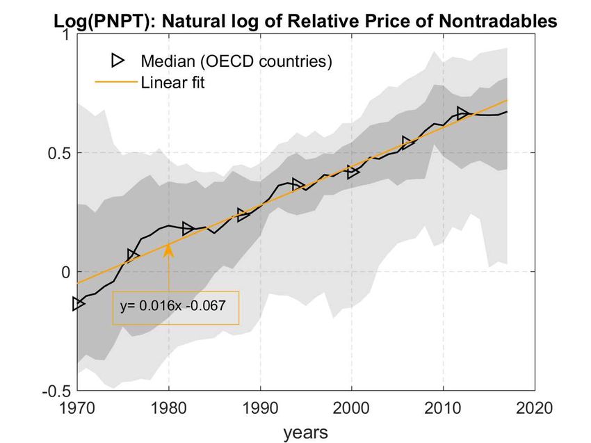
Temi di discussione
(Working Papers)

Population aging, relative prices and capital flows across the globe

by Andrea Papetti

Number 1333 - April 2021
The papers published in the Temi di discussione series describe preliminary results and
are made available to the public to encourage discussion and elicit comments.
The views expressed in the articles are those of the authors and do not involve the
responsibility of the Bank.

Editorial Board: Federico Cingano, Marianna Riggi, Monica Andini, Audinga
Baltrunaite, Marco Bottone, Davide Delle Monache, Sara Formai, Francesco
Franceschi, Adriana Grasso, Salvatore Lo Bello, Juho Taneli Makinen, Luca
Metelli, Marco Savegnago.
Editorial Assistants: Alessandra Giammarco, Roberto Marano.

ISSN 1594-7939 (print)
ISSN 2281-3950 (online)
Printed by the Printing and Publishing Division of the Bank of Italy
POPULATION AGING, RELATIVE PRICES AND CAPITAL FLOWS ACROSS THE GLOBE
                           by Andrea Papetti ∗

                                            Abstract
      This paper develops a multi-country two-sector overlapping-generations model to study
the impact of demographic change on the relative price of nontradables and current account
balances. An aging population expands the relative demand for nontradables, exerting upward
pressure on their relative price (structural transformation), and entails a willingness to save
more, as households discount higher survival probabilities, and invest less, as firms face
increasing labor scarcity. The general equilibrium reduction of the real interest rate (secular
stagnation) dampens the increase in the relative price as savings become less profitable, thus
lowering consumption at older ages. The model robustly predicts that faster-aging countries
will face greater increases in the relative price of nontradables and unprecedented
accumulations of net foreign asset positions (global imbalances) over the twenty-first century.
JEL Classification: E21, F21, J11, O11, O14.
Keywords: population aging, relative prices, capital flows, overlapping generations, tradable
nontradable, secular stagnation, structural transformation, global imbalances.
DOI: 10.32057/0.TD.2021.1333

                                                                     Contents

1. Introduction .........................................................................................................................................5
2. The model..........................................................................................................................................12
3. Calibration and solution ....................................................................................................................15
4. Validation on euro area countries: model versus data .......................................................................21
5. Understanding the sectoral mechanics of demographic change ........................................................24
6. Relative prices and capital flows in an aging world ..........................................................................31
   6.1 Calibration .................................................................................................................................31
   6.2 Main results ...............................................................................................................................33
   6.3 Sensitivity ..................................................................................................................................35
7. Sectoral reallocation and capital flows..............................................................................................42
8. Concluding remarks ..........................................................................................................................44
References ..............................................................................................................................................45
Appendix A - Set of equilibrium equations............................................................................................52
Appendix B - Expressing the initial consumption..................................................................................53
Appendix C - Solving the stationary equilibrium numerically...............................................................57
Appendix D - Calibration of the EU15 aggregate economy ..................................................................58
Appendix E - EA9 economy: additional results .....................................................................................59
Appendix F - Relative price and consumption share of nontradables: data ...........................................62
Appendix G - World economy: additional results ..................................................................................63
Appendix H - One sector model .............................................................................................................64

     ∗
         Bank of Italy, Directorate General for Economics, Statistics and Research.
[...] aging speeds up the structural transformation process since older households con- sume more services. — Cravino et al. (2020), Population Aging and Structural Transformation [...] Bernanke (2005)’s “global savings glut” has just begun. — Auclert et al. (2020), Demographics, Wealth, and Global Imbalances in the Twenty-First Century
1 Introduction1
Population aging, i.e. the process of declining fertility and mortality rates leading to increasing old
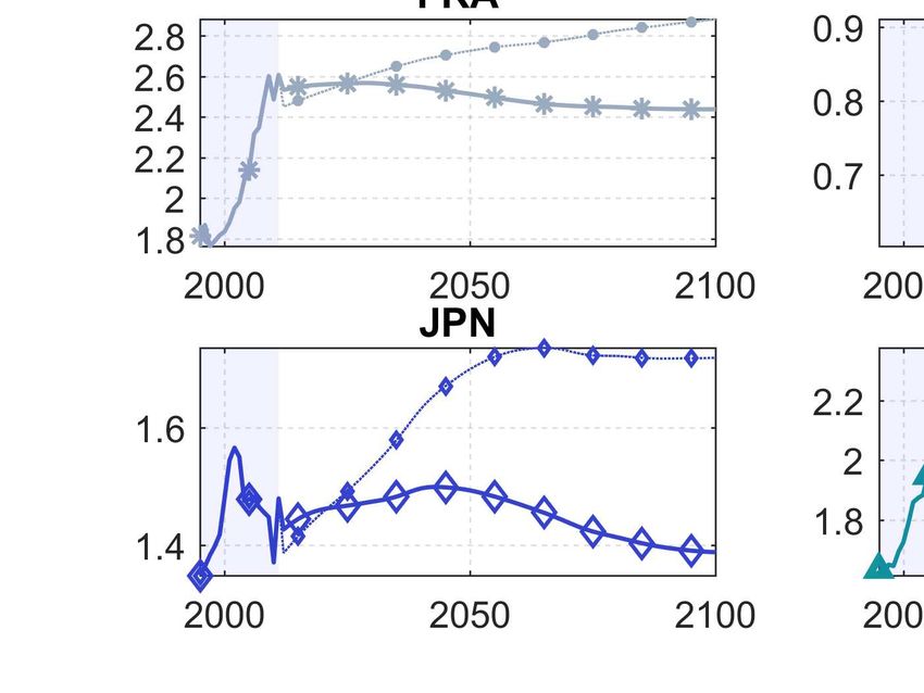
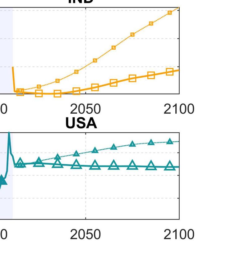
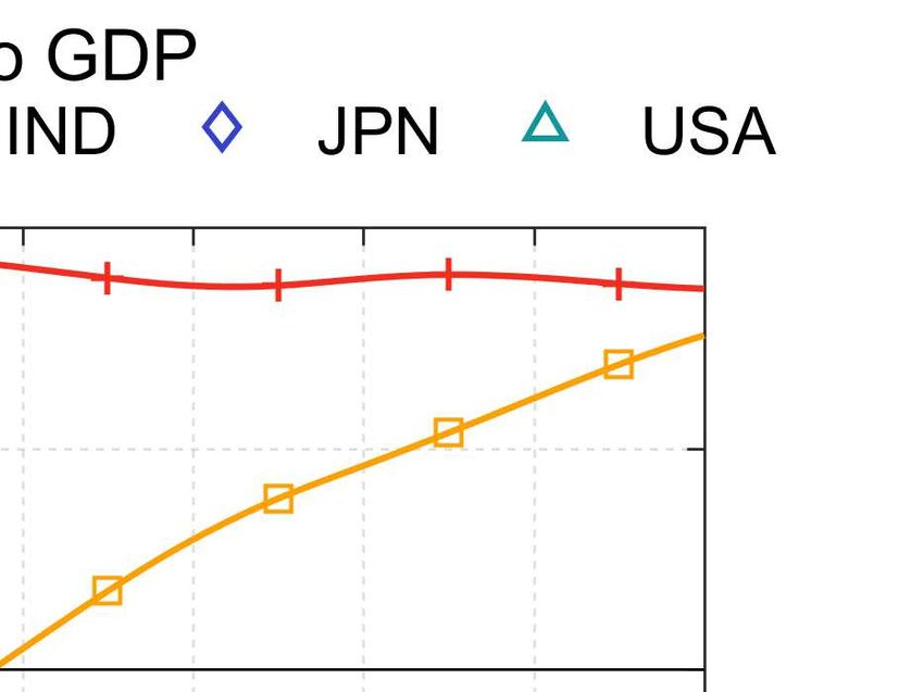
dependency ratios in all major economies (Figure 1a),2 is an underlying force of three important in-
ternational macroeconomic trends: secular stagnation (Eggertsson et al., 2019), global imbalances
(Auclert et al., 2020) and structural transformation (Cravino et al., 2020). This paper provides the
first contribution to connect these three phenomena in a multi-country dynamic general-equilibrium
quantitative model with heterogeneous agents by age, focusing the analysis on the impact of demo-
graphic change on capital flows and the relative prices of nontradable goods.
It is understood that the increasing scarcity of effective labor and longer life expectancy tend
to make capital relatively more abundant, thus bearing an environment with declining real interest
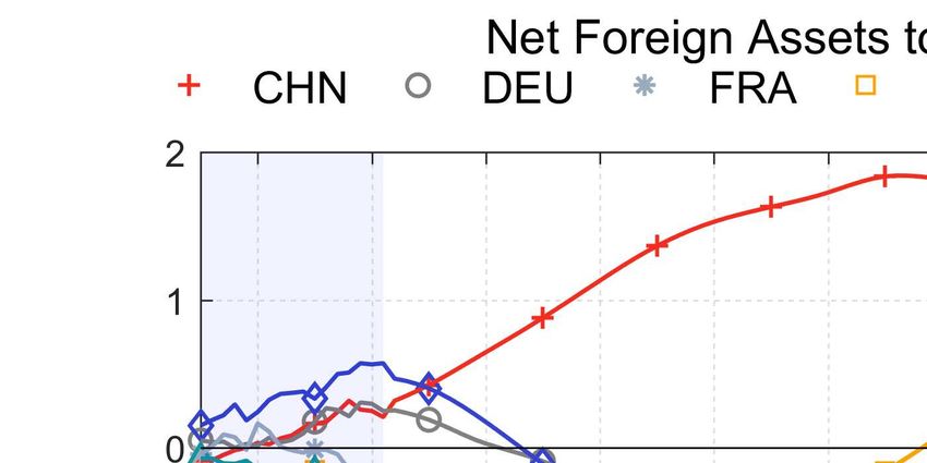
rates (secular stagnation, Figure 1b). Likewise, researchers have explored to what extent differ-
ent patterns of aging across countries can determine international capital flows in the attempt of
explaining the observed global imbalances (Figure 1c–1d). However, these studies have generally
focused on a single composite sector of the economy, thus missing a potentially important part of
why aging might matter for international macroeconomics. Namely, an older population features a
propensity to demand relatively more nontradables, thus contributing to the sectoral reallocation of
resources away from the tradable sector with an ensuing adjustment of the relative prices (structural
transformation, Figure 1e–1f).
This paper stresses the importance of considering the three macroeconomic phenomena in a
unified general equilibrium framework, for multiple reasons. First, since all countries are aging,
one could expect the same qualitative macroeconomic response to demographic change of each
country if considered as a “small-open economy” (i.e. in a partial equilibrium environment with
given real interest rate). For example, as aging tends to induce more savings and less investment one
could predict that each country runs a current account surplus – which, of course, cannot happen
at the world level. Second, in a world where all countries are willing to save more and invest less
due to aging, the real interest rate is reduced. Such a reduction, as it will be shown, could have
tangible effects on the sectoral reallocation of resources and relative prices so that, if not taken into
account, could bias the estimate of the impact of aging on structural transformation. Third, the
aging-induced sectoral reallocation could be itself a driver of capital flows and secular stagnation
– a channel that has not featured prominently into the research on the topic in spite of the original
1
For helpful comments and discussions, I thank Stefano Federico, Alberto Felettigh, Claire Giordano, Fadi Hassan,
Salvatore Lo Bello, Hannes Malmberg and seminar participants at the Bank of Italy and the European Central Bank. I
thank Zsófia L. Bárány, Nicolas Coeurdacier and Stéphan Guibaud for sharing their carefully compiled data on social
security replacement rates across the globe. I gratefully acknowledge financial support from the Bank of Italy research
fellowship for this project. All errors are my own. Disclaimer: this paper should not be reported as representing the
views of the Bank of Italy or the Eurosystem. The views expressed are my own and do not necessarily reflect those of
the Bank of Italy or the Eurosystem. First version: October 2020.
2
According to the old-dependency-ratio depicted in Figure 1a, no country is yet near to its long term level of population
aging. While the identification of a person as “old” evidently depends on a threshold that might be appropriate to
change over time, “chronological [age measured in calendar years] population aging is inevitable” (Lee, 2016).
5Old Dependency Ratio: 65+/(15-64), %
80
CHN
70 DEU
FRA
60 GBR
IND
50 ITA
JPN
40 USA
30
20
10
0
1980 2000 2020 2040 2060 2080 2100
years
(a) Population aging (b) Secular stagnation
NFA/GDP: Net Foreign Asset to GDP, % 50
80
CHN
NFA/GDP: Net Foreign Asset to GDP
40
60 DEU BEL JPN
30 DNK
IND
JPN 20 CAN
40
USA
10 CHN DEU
20 0
AUT NTL
-10 IND SWEFRA FIN
0 GBR ITA
-20
IRL USA
-20 -30 AUS
-40
-40
-50 ESP
-60 -5 0 5 10 15 20
1970 1980 1990 2000 2010 2020 ODR: Old Dependency Ratio
years
(c) Global imbalances (d) Aging-induced global imbalances
90
PNPT: relative price of nontradables
DNK
FRA ITA
70 FIN
SWE
GBR
USA NLD ESP
50
30 DEU
IRL BEL
10
AUT
JPN
-10
-5 0 5 10 15 20
ODR: Old Dependency Ratio
(e) Structural transformation (f) Aging-induced structural transformation
Figure 1: Population aging, secular stagnation, global imbalances, structural transformation
Note. (1a) The indicator in the figure is the the number of people aged more than 64 over the number of people aged
between 15 and 64. Data from the United Nations (UN, 2019) World Population Prospects 2019, Online Edition. Rev.
1, medium variant after year 2019. (1b) Trend in global real rates estimated by Del Negro et al. (2019) (DGGT) on
yield data provided by Jordá et al. (2019) (JST). The continuous line is the posterior median; shaded areas show the 68
and 95% posterior coverage intervals. Natural real interest rate estimates by Holston et al. (2017) (HLW). (1c) Data
on net foreign asset to GDP corresponding to “Estimated IIP (net of gold)/GDP” provided by Lane and Milesi-Ferretti
(2018). (1d) 1991-2018 average percentage point deviations from the 1970-1990 average. JPN and ESP are outliers.
(1e) Data on relative price of nontradables described in Appendix F. Shaded areas show the 16-84 and 2.5-97.5th
percentile ranges. (1f) 1991-2017 average percentage point deviations from the 1970-1990; JPN is outlier.
6formulation of the secular stagnation hypothesis (as noted by Lee (2016)).3 Fourth, in spite of the
common projected aging pattern, countries differ not only in terms of population size but also by
timing, extent and speed of the aging process. The interaction of such demographic differences can
play an important role not only in determining magnitude and direction of capital flows but also in
identifying those countries that can face more or less impact on their relative price of nontradables
with respect to the trading partners, hence on their real exchange rate.
The paper proceeds in three main steps. First, the developed overlapping generations (OLG)
model is described and characterized in its equilibrium dynamics. Second, the model is calibrated
with population data and projections (UN, 2019) for nine euro area countries (EA9 henceforth) to
examine if the historical data generated by the model can explain real-world capital flows and finely
measured relative prices.4 Third, the model is used for an extended set of countries – eighteen major
world economies – to make predictions of the main outcome variables in the twenty-first century.
The OLG model developed in this paper builds especially on the multi-country large-scale OLG
model of the world by Domeij and Flodén (2006) and Krueger and Ludwig (2007) to incorporate
two sectors, each producing either tradable or nontradable composite goods.5 The model has two
key distinctive features. First, consistently with the empirical evidence (Cravino et al., 2020; Gi-
agheddu and Papetti, 2018), older households have a preference to consume relatively more non-
tradables. Second, working hours are imperfectly substitutable between sectors. This latter feature
allows relative demand changes to matter for the relative price of nontradables (De Gregorio et al.,
1994) and to be consistent with the long-run persistence of sectoral hourly wage differentials found
empirically (Cardi and Restout, 2015). Countries are allowed to differ in all the main parameter
values both on the household and on the firm side in both sectors, as well as on the generosity of the
pension system. Hence the main channels in the models are mediated by a complex interconnection
of differences that contribute to the final outcome in an environment where, as it is standard in OLG
models, falling mortality (fertility) rates tend to encourage (discourage) savings (investment). To
the standard savings/investment decisions, the model adds the sectoral reallocation as a potential
driver of international capital flows.
From the perspective of the perfect-foresight OLG model, in the face of aging each country
reacts with a willingness to save more and invest less, i.e. with a willingness to run current account
surpluses. The reason is that higher survival probabilities lead agents to be willing to save more in
order to smooth consumption over a longer life. The more so the lower the generosity of the pay-as-
you-go public pension system. At the same time, constant returns to scale technology in production
means that firms are willing to demand less capital for investment as the growth rate of the effective
3
Hansen (1939) – who first formulated the secular stagnation hypothesis (Summers, 2013, 2014) – suggested that
population aging can tilt the composition of consumption demand toward services, and particularly health care, that
require relatively little capital, potentially exacerbating the problem of deficient investment demand. The OLG model
in this paper allows for such a channel.
4
The focus is on EA9 to rely on a dataset for relative prices compiled by Berka et al. (2018) with a high degree of
cross-country comparability and granularity in the tradable versus nontradable split.
5
It is a reformulation of a model first appeared in Giagheddu and Papetti (2018) as detailed in section 2.
7labor force decreases. Both factors dampen the return on capital in general equilibrium and imply
that the countries which are relatively more populous (i.e. more capital abundant), aging faster
(i.e. more willing to save), have higher effective labor productivity growth (i.e. higher economic
growth) and less generous public pension systems (i.e. less crowding-out effect on capital) tend to
develop a positive net foreign asset position over time. Sectoral allocations can play a role here,
especially given that there are sectoral differences in capital intensity.
There are three main channels in the model through which aging affects the relative price of
nontradables. First, a demand composition effect: as the population distribution tilts towards older
ages the relative demand for nontradable rises thus inducing an increase in the relative demand for
labor in the nontradable sector. To attract labor in this sector, in the presence of imperfect labor
mobility, the relative wage has to increase in turn translating into a higher relative price.
A second channel concerns the standard life-cycle consumption-savings decisions. Discount-
ing higher survival probabilities, individuals save more. For given real interest rate (i.e. in partial
equilibrium), this translates into higher expected consumption at older ages. As nontradable con-
sumption needs to be met by domestic production (while tradable consumption can be freely met
with imports from abroad), relative labor in the nontradable sector needs to increase for the non-
tradable good market to clear, and so the relative wage and the relative price of nontradables. These
two channels predict for all countries an increase of the relative price of nontradables due to aging,
in partial equilibrium. In this sense, aging can be a driver of structural transformation.6
The third channel pertains to the presence of different capital intensities between sectors. A
decrease of the rental rate of capital decreases the relative price of the product that uses capital
intensively. This effect owes famously to the Stolper and Samuelson (1941) theorem (above stated
by reversing its underlying logic) which in the current setting is “amended” because the sectoral
reallocation associated with the decrease in the rental rate of capital is mediated by a related change
in the relative wage (i.e. there is no wage equalization as in the original theorem) which, in turn,
depends crucially on the degree of sectoral labor mobility. In other words, by changing factor
prices aging might matter for the relative price of nontradables in the presence of different capital
intensities between sectors, all the more so in the presence of imperfect labor mobility.
As explained above and as well documented in the literature (see later in the introduction), aging
does decrease the real interest rate in general equilibrium. Hence the third channel above will apply
providing upward (downward) pressure on the relative price of nontradables depending on weather
6
The model in this paper allows for a non-unitary elasticity of substitution in consumption between the two composite
goods which, however, is not essential to have structural transformation led by aging. Structural transformation is
often attributed to a process where the exogenously constantly growing relative TFP in the goods sector leads to a
constantly growing relative price of services in turn associated with a growing services share in consumption as goods
and services are complements in consumption, i.e. the consumption elasticity is smaller than one (see e.g. seminal
contribution by Ngai and Pissarides (2007)). Here the mechanism through which an elasticity smaller than one might
elicit structural transformation is similar but the exogenous trigger is demographic change. Furthermore, the model in
this paper allows for differences in factor proportions between sectors, a feature deemed to be important for structural
transformation (Acemoglu and Guerrieri, 2008), while it does not allow for nonhomothetic preferences in turn deemed
to be an important feature (Boppart, 2014; Lewis et al., 2018).
8in a country the tradable sector is more (less) capital intensive than the nontradable sector. At the
same time, however, the upward pressure on the relative price of nontradables stemming from the
first two channels above will be dampened as savings become less profitable thus discouraging
consumption at later ages (which is biased towards nontradables).
The general equilibrium predictions of the model are validated on annual data for the relative
price of nontradables relative to trading partners provided by Berka et al. (2018) for the EA9 coun-
tries and on standard annual data for the current account balances to GDP (provided by the IMF
WEO). The primary quantitative exercise in the paper involves regressing these data on the corre-
sponding simulated series generated by the calibrated model. Running a fixed effect specification it
is found that the model can account for a portion of the within country variation for both the relative
prices and the current account balances, where for the latter the relevance is particularly true for
the sample periods that start between 2001 and 2007, always ending in 2020. For these sample pe-
riods the coefficient of interest is significantly close to unity, and the model explains between 15%
and 30% of the current account to GDP fluctuations, judging by the coefficient of determination
2
(Rwithin ). For the relative price of nontradables – whose data are only available for the 1995-2007
2
period – the Rwithin is about 7%. Running between and pooled OLS estimations reveal again a pos-
itive and statistically significant coefficient, very close to unity in certain cases, with a fairly high
R2 . This suggests that the model, where demographic change is the only driver, can to a certain
extent explain also level differences across countries.
Given that the model finds some validation in the empirics, it is then used to run historical
counterfactuals in order to isolate the main channels. Judged as median across the EA9 countries,
the relative price of nontradables has constantly increased by about 1.4% per annum in the data
over the 1996-2017 period.7 The model over the same period predicts an annual growth rate of
about 0.56% in partial equilibrium (i.e. at constant return to capital), that is 40% of the empirical
counterpart. Running a counterfactual where the age-varying sectoral consumption shares are fixed
at the average level prevailing until age 50, it is found that the demand composition channel (first
channel above) accounts for only about one-fifth of that 40%. Finally, in partial equilibrium all
countries are willing to run current account surpluses of about 5% of GDP, at least for the first half
of the twenty-first century. The demand composition channel does not seem to play a relevant role
for capital flows.
Turning to general equilibrium results, the return on capital decreases significantly dampening
the appreciating impact of aging on the relative price of nontradables which tends to grow by
about four-fifth less than in partial equilibrium. Therefore, it can be argued that demographic
change can account between 40% (partial equilibrium) and 8% (general equilibrium) of structural
transformation.8 For most countries the role of differences in capital intensities between sectors
7
To have the absolute level of the relative price of nontradables for each country, in this case the data source is EUK-
LEMS. The dataset on the price indices has inferior granularity compared to the one provided by Berka et al. (2018)
but extends more in time (until 2017 rather than 2007).
8
When structural transformation is judged by the nontradable share of consumption, demographic change can account
9(third channel above) explains around a fourth of the general equilibrium absolute deviation of the
relative price of nontradables from the initial level. Overall, the dynamics of capital flows is not
strongly influenced by sectoral reallocation while standard consumption-savings decisions are key.
Finally, when the model is extended to have a world economy with eighteen countries covering
about 70% of world GDP, 60% of trade (i.e. exports of goods and services) and 50% of world
population, the most striking result is that, consistently with Auclert et al. (2020), the model predicts
China and India to become the sole countries with a positive net foreign asset position over the
twenty-first century. These countries are populous (covering and projected to cover together more
than 70% of the world population considered in the model) and are expected to age faster than the
trading partners (see Figure 1), hence with a greater willingness to accumulate savings. Since these
countries are also those that the model predicts to have the biggest demographics-induced growth
of labor productivity (GDP per unit of effective labor employed), demographic change features as
a factor that can alleviate the “allocation puzzle” (Gourinchas and Jeanne, 2013), as also noticed by
Bárány et al. (2019) and Sposi (2019).9 The model of this world economy predicts a clear positive
relationship between the growth rate of the old-dependency ratio and the growth rate of the relative
price of nontradables, both in partial and general equilibrium, thus confirming existing empirical
estimates (Groneck and Kaufmann, 2017).
Related literature. The macroeconomic impact of demographic change is certainly a long-
standing issue (Lee (2016) for a review). Recently, the revival of Hansen (1939)’s “secular stagna-
tion” hypothesis – thanks to Summers (2013, 2014) – has fostered macroeconomic research mostly
focused on the impact of aging on the (natural) real interest rate and output, analyzing primarily
closed economies with OLG models in the spirit of Auerbach and Kotlikoff (1987) (Gagnon et al.
(2016), Eggertsson et al. (2019), Bonchi and Caracciolo (2020) for the US, Cooley et al. (2019),
Bielecki et al. (2020), Papetti (2020) for Europe, Sudo and Takizuka (2019) for Japan, Cooley and
Henriksen (2018) for US and Japan); or in the spirit of Gertler (1999)’s simpler life-cycle model
(Carvalho et al. (2016) for a representative OECD economy, Kara and von Thadden (2016) for euro
area, Rachel and Summers (2019) for a world economy modeled as a unique block). These models
tend to robustly predict a downward impact of population aging on output and return on capital,
similarly to the framework here developed.10
Mutli-country one-sector OLG models have been widely used to study capital flows. Here
between 19% (partial equilibrium) and 10% (general equilibrium) of the observed variation in the median nontradable
share of consumption between 1995 and 2015 (as reported in Table 4, cf. Figure E.4). Comparably, by means of
an empirical decomposition based on Boppart (2014)’s theoretical structure, Cravino et al. (2020) find for the United
States that “changes in the age-structure of the population accounted for 20% of the observed change in the service
expenditure share over this period [1982–2016]”.
9
A standard neo-classical growth model predicts that countries enjoying higher productivity growth should receive
more net capital inflows. A prediction that does not square with the data and has been therefore labeled ‘allocation
puzzle” by Gourinchas and Jeanne (2013). Cf. Lucas (1990); Prasad et al. (2007).
10
Challenges to such a prediction have been provided in modeling frameworks where the increasing scarcity of labor
induced by aging can be compensated by human capital formation (Fougère and Mérette, 1999; Ludwig et al., 2012)
and by the adoption of automation technology (Acemoglu and Restrepo, 2017, 2018; Basso and Jimeno, 2020).
10the main references are: Brooks (2003), Domeij and Flodén (2006), Krueger and Ludwig (2007),
Attanasio et al. (2007), Backus et al. (2014); and more recently: Bárány et al. (2019), Auclert et al.
(2020). Compared to them, the paper exhibits a two-sector model that hence makes possible to
study sectoral reallocation as well as relative prices. Rausch (2009) (chapter 4) is an exception in the
literature, employing a fully-fledged OLG model with multiple sectors. The focus, however, is on a
single country (Germany) modeled as a closed-economy. Galor (1992) is the seminal contribution
in the literature that paved the way to the resolution of two-sector OLG models that, however, have
been rarely used in an open-economy setting (Bajona and Kehoe (2006); Mountford (1998); Naito
and Zhao (2009); Sayan (2005) have all kept analytical tractability to the detriment of capturing the
full age-structure of the population).11
Some empirical work has studied the impact of the relative demand shift caused by aging on
structural transformation (Börsch-Supan, 2003; Cravino et al., 2020), specifically on the relative
price of nontradables (Groneck and Kaufmann, 2017) and on the real exchange rate (Giagheddu
and Papetti, 2018). This last reference offers also the main theoretical framework which the model
in the paper has built upon, extending the two-country static analysis there in a dynamic multi-
country analysis with additional degrees of heterogeneity at both the secotral and country levels.
Essentially, by adding two sectors to the frontier multi-country large scale overlapping gener-
ations (OLG) models, this paper bridges two strands of the literature in international macroeco-
nomics. On the one hand, those contributions that study the impact of demographic change on
capital flows in a one-sector OLG model, cited above. On the other hand, those contributions that
study the long-term determinants of relative prices, with focus on tradables versus nontradables,
that have thus far mostly focused on models with a single representative agent that cannot take into
account the permanent nature of certain changes such as those brought about by aging. Within
this latter wide set of contributions, Berka et al. (2018) (and the references therein) offer a closely
related assessment with a focus on the evolution of sectoral productivity in the euro area; Cardi
and Restout (2015) offer the main evidence in support of the long-run persistence of sectoral wage
differentials, at the heart of the theoretical framework here developed.
The rest of the paper is organized as follows. Section 2 presents the model. Section 3 describes
how to calibrate and solve the model. Section 4 compares relative prices and capital flows implied
by the model with real-world data for nine euro area countries. Section 5 runs historical counter-
factuals to isolate the main channels. Section 6 extends the analysis to eighteen countries covering
about 70% of world GDP to make predictions into the twenty-first century. Section 7 explores the
relationship between capital flows and sectoral reallocation. Section 8 concludes.
11
The focus of the present analysis in studying capital flows and hence global imbalances is uniquely on the contribution
of demographic change. Obviously, this does not exclude concurrent explanations such as e.g. different levels
of financial development across countries that might translate into a different strength of the precautionary saving
motive (Mendoza et al., 2009) as surveyed in Gourinchas and Rey (2014).
112 The model
This section presents a multi-country overlapping-generation (OLG) neoclassical growth model
that expands on the work by Domeij and Flodén (2006) and Krueger and Ludwig (2007) to in-
corporate two sectors. It is a reformulation of a model first appeared in Giagheddu and Papetti
(2018).12 Each country is populated by overlapping generations of households that solve a life-
cycle consumption problem. Only two goods are produced and consumed: a composite tradable
(T) good that can be freely shipped between countries and serves as numeraire, and a composite
nontradable (N) good that cannot leave the country in which it is produced. The production tech-
nology is identical between countries and sectors, while it can differ in its parameter values. Labor
is immobile while capital can perfectly move between countries. The model is purely real, abstract-
ing from nominal frictions. The demographic variables are exogenous. One period corresponds to
one year. The two distinctive features of the model are: (a) age-dependent sectoral consumption
shares; (b) imperfect labor mobility between sectors.
Households. Each household consists of a single individual. Households within each cohort
j are identical and their exogenous mass Ni,t,j for time-period t in country i evolves recursively
according to:
Ni,t,j = Ni,t−1,j−1 si,t,j (2.1)
where si,t,j is the conditional survival probability.13
For each period t the life-cycle problem is such that the representative household born in t
chooses consumption in each sector cN T
i,t+j,j , ci,t+j,j and the amount of assets to hold the sequent pe-
riod ai,t+j+1,j+1 for each age j ∈ {0, 1, 2, · · · J} under the assumption of perfect domestic annuities
market;14 how to allocate in each sector an exogenously given amount of hours to work, ht+j,j , for
12
Aside from considering more than two countries and the transition dynamics, the main difference with that version
is to allow for non-unitary elasticity of substitution both in intertemporal consumption and between the two goods
consumption, further allowing for differences across countries and between sectors in the capital-output ratios and in
the factor intensities.
13
Given that an individual is aged j − 1 at time t − 1, si,t,j is the probability to be alive at age j at time t in country
i. Following Domeij and Flodén (2006), data are taken for Ni,t,j for each considered i, t, j to get the implied
survival probabilities si,t,j which therefore can exceed 1 due to migration flows. The underlying assumption is
that immigrants enter the economy without assets and are adopted by domestic households: assets are carried over
between periods by a domestic cohort and then split among its survivors and the asset-less immigrants in the same
age class.
14
The assumption of “perfect annuities market” means that the agents within each age group j agree to share the assets
of the dying members of their age group among the surviving members. Using the notation just introduced, consider
those that at time t are aged j (omit the country index i for simplicity). The total amount of assets of the dying
members is: at,j (1 − st,j )Nt−1,j−1 , while the number of surviving members is: Nt,j = Nt−1,j−1 st,j . Hence, in
the budget constraint the asset holding in period t + 1 will depend on what as been accumulated plus this sort of
‘equal gift’ from the dying members given the real interest rate (rt ) at which these assets can be invested (minus
12each age j ∈ {0, 1, 2, · · · jr } choosing hN T
i,t+j,j , hi,t+j,j , solving the following problem:
( J )
X
j
c1−σ
t+j,j
max β πt+j,j (2.2)
cN T N T
i,t+j,j ,ci,t+j,j ,hi,t+j,j ,hi,t+j,j ,ai,t+j+1,j+1 j=0
1−σ
subject to
φφ+1
i
− φ1 φi +1
− φ1
φi +1 i
ci,t+j,j = αi,j i (cTi,t+j,j ) φi
+ (1 − αi,j ) i (cN
i,t+j,j )
φi
(2.3)
ε ε+1
i
− ε1 εi +1
− ε1
εi +1 i
hi,t+j,j = θi i
(hTi,t+j,j ) εi
+ (1 − θi ) i (hN
i,t+j,j )
εi
(2.4)
ai,t+j,j (1 + rt+j )
ai,t+j+1,j+1 = N
− cTi,t+j,j − Pi,t+j cN
i,t+j,j + yi,t+j,j (2.5)
si,t+j,j
N
yi,t+j,j = (1 − τi,t+j )(wi,t+j hN T T
i,t+j,j + wi,t+j hi,t+j,j )I(j < Ji ) + di,t+j,j I(j ≥ Ji )(2.6)
ai,t+J+1,J+1 = 0 (2.7)
ai,t,0 = 0 (2.8)
where πi,t+j,j = jk=0 si,t+k,k represents the unconditional survival probability with si,t,0 = 1
Q
for all i, t; β is the discount factor; I(·) is an indicator function where Ji denotes the exogenous
retirement age; di,t+j,j denotes the pension benefit. Prices (taken as given by the household) are:
T N N
wi,t , wi,t , rt , Pi,t denoting the real wage in the tradable and non-tradable sector, the real interest rate
on assets, and the the relative price of nontradables respectively. The household’s labor supply in
efficiency units, hi,t+j,j = hi,j , is exogenous and depends on age but is constant over time.15
The two distinctive features of the model are represented by constraints (2.3) and (2.4): the
parameter 0 < αi,j < 1 denotes the age-dependent share of consumption expenditure devoted to
tradables; with 0 < θi < 1, the parameter εi denotes the degree of substitutability between hours
supplied in the two sectors (both at the individual and at the aggregate level) with the case of perfect
labor mobility represented by εi → ∞; correspondingly, εi → 0 represents immobility.16
consumption plus income):
at,j (1 + rt )(1 − st,j )Nt−1,j−1 at,j (1 + rt )
at+1,j+1 = at,j (1 + rt ) + − ct,j + yt,j = − ct,j + yt,j
Nt−1,j−1 st,j st,j
which is the budget constraint written in the main text.
15
Particularly, it varies by age in accordance with productivity and labor market participation by age similarly to what
assumed in Domeij and Flodén (2006).
16
This modeling choice of sectoral hours serves the main purpose of allowing demand factors (such as the change
in demand composition induced by aging) to influence relative prices, coherently with the empirical finding that
wages tend not to be equalized between sectors in the long-run (Cardi and Restout, 2015). It amounts to assuming
that households have a preference to diversify labor despite wage differences between sectors. It can be thought
to broadly capture structural forces in an economy, including compositional differences of the work-force between
sectors, that might be responsible for the long-run persistence of sectoral wage differences detected in the data.
In neoclassical models with perfect factor mobility the long-run relative price of nontradables is independent of
13Firms. The representative firm in each sector s ∈ {T, N } and in each period t hires (hours in
efficiency units of) labor Lsi,t at a given hourly wage rate wi,t s s
and rents capital Ki,t at price rt (real
interest rate) subject to yearly depreciation rate δi so as to solve:
s ψis s
s
max
s s
Pi,t (Ki,t ) (Zis Lsi,t )1−ψi − wi,t
s
Lsi,t − (rt + δi )Ki,t
s
(2.9)
Ki,t ,Li,t
T
where Pi,t is normalized to unity for all i, t, 0 < ψis < 1 is the output elasticity to capital and Zis is
the sector-specific labor-augmenting technology.
Government. Given a certain level of generosity of the pay-as-you-go (PAYG) pension system,
i.e. the replacement rate d¯i defined as the pension benefit di,t received by each household per unit
of the average labor income wi,t (1 − τi,t )h̄i , the government sets a tax rate τi,t such that its budget
is balanced in each period:17
di,t = d¯i wi,t (1 − τi,t )h̄i (2.10)
X J
τi,t wi,t Li,t = di,t Ni,t,j (2.11)
j=J
1
, Li,t = Jj=0 hi,j Ni,j .
T 1+εi N 1+εi 1+εi
P
where wi,t = θi (wi,t ) + (1 − θi )(wi,t )
Clearing. The labor market in each sector s ∈ {T, N } and the market for nontradables clear in
each period t:
J
X
Lsi,t = hsi,t,j Ni,t,j (2.12)
j=0
J
N N
X
N ψi
(Ki,t ) (ZiN LN
i,t )
1−ψi
= Ni,t,j cN
i,t,j (2.13)
j=0
The international capital market clears:18
X XX
T N
Ki,t+1 + Ki,t+1 = ai,t+1,j+1 Ni,t,j (2.14)
i i j
Equilibrium. Given the exogenous demographic development (fully characterized by the in-
coming cohort size Nt,0 and the conditional survival probabilities st,j according to (2.1)) in all
consumer demand patterns (see Obstfeld and Rogoff (1996), ch. 4). There are other ways to allow for demand factors
to matter (e.g. having diminishing returns to scale in at least one sector (Galstyan and Lane, 2009); or assuming that
an economy is partially shut off from world capital markets (Froot and Rogoff, 1994)). This modeling choice owes to
its intuitiveness and close link with some recent literature. Giagheddu and Papetti (2018) provide further elaborations
on this assumption. Other works employing a CES aggregator to capture imperfect sectoral labor mobility include:
Horvath (2000), Kim and Kim (2006), Bouakez et al. (2009), Iacoviello and Neri (2010), Bouakez et al. (2011),
Altissimo et al. (2011), Cardi and Restout (2015), Groneck and Kaufmann (2017), Cantelmo and Melina (2018).
17
PJi −1
Have: h̄i = j=0 hi,j /Ji .
18
By Walras’ law the world market for the tradable good clears too (a superfluous condition in terms of computation
once all the conditions above are satisfied).
14periods t = 0, 1, ..., ∞, for all cohorts j = 0, 1, ..., J for all considered countries i, the equi-
T N N ∞
librium for this (perfectly competitive) economy is a sequence of prices wi,t , wi,t , Pi,t , rt t=0 ,
∞
n
J
o∞
, policies {τi,t }∞
T N
T
quantities Ki,t , Ki,t , LTi,t , LN
i,t t=0 , ci,t,j , cN T N
i,t,j , hi,t,j , hi,t,j , ai,t,j j=0 t=0 and
t=0
transfers {di,t }∞
t=0 such that:
1. households solve the optimization problem (2.2) subject to constraints (2.3)–(2.8);
2. firms maximize profits solving problem (2.9);
3. the fiscal authority sets a tax rate (2.11) such that its budget is balanced in each period given
the individual pension transfer (2.10);
4. factor markets (2.12), the nontradable good market (2.13) and the international capital market
(2.14) clear.
Capital flows. The net foreign asset position of a country (Fi,t ) and its change, namely the
current account (CAi,t ), are auxiliary variables stemming from the difference between the national
N T
P
capital supply, Ai,t ≡ j ai,t+1,j+1 Ni,t,j , and demand, Ki,t ≡ Ki,t + Ki,t :
Fi,t+1 = Ai,t − Ki,t+1 (2.15)
CAi,t = Fi,t+1 − Fi,t (2.16)
P
By (2.14), it must be: i CAi,t = 0. In the reminder, the main variable of interest will be the
current account relative to the gross domestic product (GDPi,t ):
CAi,t
cai,t = (2.17)
GDPi,t
s s
N N
where GDPi,t = Yi,tT + Pi,t s ψi
Yi,t , Yi,ts = (Ki,t s
) (Zi,t Lsi,t )1−ψi for s ∈ {T, N }.
3 Calibration and solution
The goal of the subsequent quantitative analysis is to study the transition dynamics of the macroe-
conomic system of section 2 from an initial to a final stationary equilibrium, where the unique
perfectly-anticipated exogenous driving process is the time-varying demographic structure. The
main focus is on two outcomes: the relative price of nontradables and the current account.
Experiment. Embracing the working hypothesis of Berka et al. (2018) – who postulate that
a common currency is a fertile ground for finding evidence on the role of fundamentals (their
priority is sectoral productivity) on the relative price of nontradables (thus on the real exchange
rate) – the model economy consists of the same nine euro area countries (EA9 henceforth) in their
15analysis, which are assumed to compose a closed economy and will serve to evaluate the model’s
performance to explain real-world data since the 1995 (when the dataset they complied starts).19
One period of the model corresponds to one year. It is assumed that in the initial stationary equi-
librium the system has the demographics prevailing in year 1996 in the data.20 Following Domeij
and Flodén (2006), equation (2.1) is directly used to retrieve the conditional survival probabilities
using data on the number of people, Nt,j , by single age-group j for each year t (the time-range
available is: 1950-2100). Data are taken from the United Nations (UN, 2019) World Population
Prospects 2019, Online Edition. Rev. 1, including the medium variant projections until year 2100.
The experiment is such that while in 1995 (as well as in all previous periods) the system is
assumed to be in the initial stationary equilibrium, in 1996 there is the information shock: agents
learn about the new demographic development for all subsequent years, and what this implies for
macroeconomic variables in a perfect-foresight environment. In year 2100 the conditional survival
probabilities and the incoming cohort size start remaining fixed forever. This implies an evolution
of the demographic structure that eventually gets stationary again.21
Given the demographics, the structural model parameters and the implied solution values for
the initial and final stationary equilibrium, the dynamic equilibrium is solved using a standard
deterministic simulation set-up where the numerical problem of solving a nonlinear system of si-
multaneous equations is managed by means of a Newton-type method.22
Common parameters. Table 1 summarizes the model parameters whose value is assumed to
be equal across countries. In line with the main references on multi-country general equilibrium
OLG models, the discount factor, β, is set to 0.9606 (or 0.99 at the quarterly frequency) – see e.g.
Bárány et al. (2019); the inverse of the elasticity of intertemporal substitution (e.i.s.), σ, is set to
2 (see e.g. Attanasio et al. (2007); Bárány et al. (2019); Domeij and Flodén (2006)).23 The labor
augmenting technology in the nontradable sector, Z N , is normalized to one so that Z T will identify
the (country-specific) relative labor augmenting technology of the tradable sector.
For what concerns demographics, it is assumed that households enter the world as workers at
age 15, all retiring at age 65 which correspond to J = 50 (this implies that hj drops abruptly to zero
19
EA9 is composed by the following countries: Austria (AUT), Belgium (BEL), Germany (DEU), Spain (ESP), Finland
(FIN), France (FRA), Ireland (IRL), Italy (ITA), Netherlands (NLD).
20
That is, for all j = 0, 1, ..., J − 1 the demographic structure is given by: N1996,j+1 = π1996,j+1 N1996,0 .
21
Therefore, population growth is zero in both the initial and final stationary equilibrium.
22
To solve for the transition dynamics, an algorithm can be designed, in the spirit of e.g. Krueger and Ludwig (2007)
or Attanasio et al. (2007), where one needs to guess the paths of the world real interest and the country-specific
N
relative price of nontradables (Pi,t , ∀i, t), once solved for the initial and final stationary equilibrium. The full set
of equilibrium equations in Appendix A makes it evident. In practice, the solution method can be handled under
the “perfect foresight solver” available in Dynare, solving separately for the initial and final stationary equilibrium.
Specifically, the Jacobian of the system has dimension 3934 × 400 given that there are 437 endogenous variables
for each of the 9 countries plus the real interest rate which is common to all countries over 400 periods (years).
Therefore, the terminal period is year 2395, which is more than sufficiently far into the future for the model to reach
the final stationary equilibrium.
23
As noted by Bárány et al. (2019), σ = 2 is in the mid-range of empirical estimates. The reader is redirected there for
the main empirical references.
16after age 64). This is a standard assumption based on the reported retirement ages for European
economies (see Carvalho et al. (2016), Table 2). Households live at most until age 99 corresponding
to J = 84 so that in each year there are 85 overlapping generations. The individual labor supply
in efficiency units, hj , is interpolated using the data-points provided by Domeij and Flodén (2006),
obtained by interacting the profiles of both productivity and the participation rates allowing the
age-labor income profile from the model to be consistent with its empirical counterpart (see Figure
2a and the note therein).24 The age-varying share parameter in the CES consumption aggregator
(2.3) is assigned values from the empirical consumption shares in tradable goods inferred from the
US Consumer Expenditure Survey (CEX), where a cubic interpolation is adopted for missing data
on extreme age-bins. The note under Figure 2b details the tradable versus nontradable classification
adopted while further details and analyses hinging upon the CEX-based dataset complied by Aguiar
and Hurst (2013) are provided in Giagheddu and Papetti (2018).25 It is apparent that while the share
of consumption devoted to nontradables is fairly constant between ages 15 and 60, after age 60 it
increases dramatically. On average, a person aged 85 has nontradable share in the consumption
basket which is about 15 percentage points bigger than a person aged 50.26
Table 1: Baseline calibration: common parameters across countries
Parameter Value Description Source
β 0.994 discount factor standard, e.g. Bárány et al. (2019)
σ 2 inverse e.i.s. standard, e.g. Domeij and Flodén (2006)
ZN 1 NT productivity normalization
J age 65 retirement age Tab. 2 in Carvalho et al. (2016)
hj Figure 2a labor supply efficiency Domeij and Flodén (2006), Hansen (1993)
αj Figure 2b T consumption share Giagheddu and Papetti (2018), Aguiar and Hurst (2013)
Country-specific parameters. As summarized in Table 2, the values of the main parameters
determining the sectoral allocations are taken from Bertinelli et al. (2020) (see their Table 4) who
update the analysis in Cardi and Restout (2015) (see their Table 5) with a more recent release of
EUKLEMS data.27 Specifically, the intra-temporal sectoral elasticities of substitution in consump-
tion, ϕ, and in labor supply, ε, are structurally estimated deriving testable equations rearranging the
24
Following a common assumption in OLG modeling (that can be found in most of the literature mentioned in this
paper), labor force participation rates are assumed to be constant over time. Hence, the model is not tailored to
directly capture structural changes such as the increase in female labor force participation.
25
While some data on age-varying consumption shares by sector are available for some European countries (cf. Gi-
agheddu and Papetti (2018)), the US data were preferred due to their higher level of detail.
26
This feature is robust to different years of analysis and to a different, more disaggregated, classification of the con-
sumption categories into tradable and nontradable as proven by the marked-black line in Figure 2b. It closely resem-
ble the age-varying consumption pattern found by Cravino et al. (2020), based on CEX data too, where the focus is
on services versus goods rather than on nontradables versus tradables.
27
Bertinelli et al. (2020) employ a sectoral concordance between the March 2011 and July 2017 releases (including
also data for Canada and Norway from the OECD STAN database), where the former provides data for eleven 1-digit
ISIC-rev.3 industries over the period 1970-2007 while the latter provides data for thirteen 1-digit-rev.4 industries over
the period 1995-2013 (see Table F.1 in Appendix E). The structural parameter estimation is conducted on a panel of
17 OECD countries with annual data running from 1970 to 2013.
17Age-income profile
0.5
1.2
data
model 0.45
1
0.4
0.8 0.35
0.3
0.6
0.25
0.4
0.2
0.2 0.15
15 25 35 45 55 65 75 85 95
age
0
0 10 20 30 40 50 60 70 80 90 CEX 2015 - cubic interpolation CEX 1980-2003 - regression estimation
age
(a) (b)
Figure 2: Age dependent: age income profile (wEA9 hj ) and tradable shares of (private) consump-
tion expenditure (αj )
Note. Panel (a). The labor supply in efficiency units (hj ) is obtained as cubic interpolation on data points provided
in Domeij and Flodén (2006). These data points are the product of participation rates provided by Fullerton (1999)
and productivity provided by Hansen (1993). The figure shows hj multiplied by the simple average across countries
of the wage rate prevailing in the initial steady state (wEA9 ), then normalized on the mean for persons 50-60 years old.
The empirical counterpart is the “smooth mean” of the labor income series provided by the National Transfers
Accounts (NTA), cf. Lee and Mason (2011), presented as median of the available countries. The European countries
for which data is available are (year used in parenthesis - often only one year is available, results are not sensitive
to the specific year used): Austria (2005), Finland (2004), France (2005), Germany (2003), Italy (2008), Spain
(2000). Panel (b). US data source: Consumer Expenditure Survey (CEX). The continuous grey line is a cubic
interpolation on CEX, 2015, “Table 1300. Age of reference person: Shares of annual aggregate expenditures and
sources of income” from which the average private consumption expenditure (measured in millions of US dollars)
is computed. The following categories are classified as tradable: food at home, alcoholic beverages, furnishings
and equipment, apparel and services, transportation, tobacco products and smoking supplies; as nontradable: food
away from home, housing minus furnishings and equipments, healthcare, entertainment, personal care products
and services, reading, education. The marked black line reports the estimated coefficient values on the constant
and age dummies of an OLS regression of the share of consumption on tradables on a constant, age dummies and
(normalized) year dummies. The dataset employed is complied by Aguiar and Hurst (2013) based on the multiple
cross-sections of households of CEX for all years between 1980 and 2003. The 49 consumption categories are
classified into tradable and non-tradable with further details and analyses in Giagheddu and Papetti (2018).
optimal rules deriving from the aggregate versions of the CES aggregators (2.3), (2.4). The sectoral
capital shares of income, ψ T and ψ N , are obtained as complements of the respective average labor
share of income (i.e. the ratio of labor compensation to value added).28 The share parameter in the
CES aggregator (2.4) is obtained as average tradable share in hours worked.
To calibrate the social security systems in all countries, measures of the effective replacement
¯ provided (and kindly shared) by Bárány et al. (2019) were adopted. These measures
rates, d,
28
Labor compensation is total labor costs that include compensation of employees and labor income of the self-
employed and other entrepreneurs.
18upgrade the official replacement rates to take into account concerns about measurement errors
or potential biases in the percentages of retirees receiving benefits and working-age population
contributing to pensions.29
Table 2: Baseline calibration: country-specific parameters
Country Empirical target Parameter
(pop share) K/Y QN δ ZT ψT ψN θ ϕ ε d
rel. N rel. T T N T T/N T/N
capital capital pension
price pro- capital capital share consum. labor
-output deprec. replacem.
rel. to duc- share of share of in elas- elas-
ratio rate rate
EU15 tivity income income labor ticity ticity
AUT (0.03) 1.97 0.97 0.10 1.41 0.32 0.32 0.40 1.52 1.10 0.65
BEL (0.04) 1.76 1.06 0.12 1.82 0.34 0.33 0.36 1.24 0.61 0.43
DEU (0.29) 1.92 1.16 0.09 2.06 0.24 0.36 0.40 0.58 1.01 0.31
ESP (0.14) 1.53 0.95 0.18 1.34 0.40 0.34 0.40 1.39 1.02 0.59
FIN (0.02) 2.18 1.07 0.07 1.32 0.35 0.26 0.42 0.85 0.43 0.67
FRA (0.21) 1.87 1.14 0.09 1.80 0.28 0.31 0.36 0.89 1.40 0.40
IRL (0.01) 1.66 0.95 0.19 1.22 0.49 0.31 0.42 1.35 0.22 0.23
ITA (0.21) 1.75 0.93 0.10 1.30 0.26 0.33 0.42 0.72 1.66 0.58
NLD (0.06) 1.79 1.09 0.11 1.45 0.39 0.26 0.33 0.52 0.22 0.25
EA9 (1.00) 1.82 1.04 0.12 1.52 0.34 0.31 0.39 1.01 0.85 0.46
Source WDI Berka et al. implied Bertinelli et al. (2020) Bárány et al.
Note. The population shares in parenthesis refer to year 1995. EA9 reports the simple average.
Given the assigned values to the common parameters across countries summarized in Table
¯ as well as the initial demographic
1 and to the country-specific parameters {ψ T , ψ N , θ, ϕ, ε, d},
structure, the calibration procedure involves solving numerically the initial stationary equilibrium
for the real interest rate as well as for the country-specific capital depreciation rate, δ, and the
relative labor augmenting technology of the tradable sector, Z T , to target the empirical capital-
output ratios and the initial relative prices of nontradables.
As mentioned above, the empirical counterpart for the relative prices of nontradables comes
from the series complied by Berka et al. (2018) which covers, at the annual frequency, the period
1995-2007, and that was chosen because of its high degree of detail in the items composing the
consumer’s basket determining the sectoral price level indices.30 A complication arises because
this series is measured in relative terms with respect to the average across 15 European countries
29
A measure for Ireland was missing in Bárány et al. (2019) and was constructed following their methodology. Particu-
larly, the “share of population above legal retirement age in receipt of a pension” (0.647) and the “active contributors
to a pension scheme in the working age population” (0.639) from the ILO (2010) Tab. 21 were averaged to multi-
ply the official “net replacement rate” (0.359) reported in the OECD database. Bárány et al. (2019) report that the
measure of the official replacement rate by the OECD (which does not distinguish between social security benefits
and alternative pension schemes) correlates very highly (above 0.8) with the measure they developed for European
countries, justifying its adoption here.
30
The series is based on data provided by Eurostat as part of the Eurostat-OECD PPP Programme where price level
indices are available for 146 “basic headings” of consumer goods and services covering 100 of the consumption
basket. Their online Appendix details the data construction including the breakdown into tradable vs nontradable
(see their Table A1). The series used here is what in their paper is labeled as qn .
19You can also read