A Lagrangian approach towards extracting signals of urban CO2 emissions from satellite observations of atmospheric column CO2 (XCO2): X-Stochastic ...
←
→
Page content transcription
If your browser does not render page correctly, please read the page content below
Geosci. Model Dev., 11, 4843–4871, 2018
https://doi.org/10.5194/gmd-11-4843-2018
© Author(s) 2018. This work is distributed under
the Creative Commons Attribution 4.0 License.

A Lagrangian approach towards extracting signals of urban CO2
emissions from satellite observations of atmospheric column CO2
(XCO2): X-Stochastic Time-Inverted Lagrangian Transport model
(“X-STILT v1”)
Dien Wu1 , John C. Lin1 , Benjamin Fasoli1 , Tomohiro Oda2 , Xinxin Ye3 , Thomas Lauvaux3 , Emily G. Yang4 , and
Eric A. Kort4
1 Department  of Atmospheric Sciences, University of Utah, Salt Lake City, USA
2 Goddard  Earth Sciences Technology and Research, Universities Space Research Association, Columbia, Maryland/Global
Modeling and Assimilation Office, NASA Goddard Space Flight Center, Greenbelt, Maryland, USA
3 Department of Meteorology and Atmospheric Science, Pennsylvania State University, USA
4 Climate and Space Sciences and Engineering, University of Michigan, Ann Arbor, USA

Correspondence: Dien Wu (dien.wu@utah.edu)

Received: 5 May 2018 – Discussion started: 14 June 2018
Revised: 22 September 2018 – Accepted: 22 October 2018 – Published: 4 December 2018

Abstract. Urban regions are responsible for emitting signif-      Orbiting Carbon Observatory 2 (OCO-2) XCO2 data. X-
icant amounts of fossil fuel carbon dioxide (FFCO2 ), and         STILT incorporates satellite profiles and provides compre-
emissions at the finer, city scales are more uncertain than       hensive uncertainty estimates of urban XCO2 enhancements
those aggregated at the global scale. Carbon-observing satel-     on a per sounding basis. Several methods to initialize re-
lites may provide independent top-down emission evalua-           ceptor/particle setups and determine background XCO2 are
tions and compensate for the sparseness of surface CO2 ob-        presented and discussed via sensitivity analyses and compar-
serving networks in urban areas. Although some previous           isons. To illustrate X-STILT’s utilities and applications, we
studies have attempted to derive urban CO2 signals from           examined five OCO-2 overpasses over Riyadh, Saudi Arabia,
satellite column-averaged CO2 data (XCO2 ) using simple           during a 2-year time period and performed a simple scal-
statistical measures, less work has been carried out to link      ing factor-based inverse analysis. As a result, the model is
upwind emission sources to downwind atmospheric columns           able to reproduce most observed XCO2 enhancements. Er-
using atmospheric models. In addition to Eulerian atmo-           ror estimates show that the 68 % confidence limit of XCO2
spheric models that have been customized for emission esti-       uncertainties due to transport (horizontal wind plus vertical
mates over specific cities, the Lagrangian modeling approach      mixing) and emission uncertainties contribute to ∼ 33 % and
– in particular, the Lagrangian particle dispersion model         ∼ 20 % of the mean latitudinally integrated urban signals,
(LPDM) approach – has the potential to efficiently determine      respectively, over the five overpasses, using meteorological
the sensitivity of downwind concentration changes to upwind       fields from the Global Data Assimilation System (GDAS).
sources. However, when applying LPDMs to interpret satel-         In addition, a sizeable mean difference of −0.55 ppm in
lite XCO2 , several issues have yet to be addressed, including    background derived from a previous study employing simple
quantifying uncertainties in urban XCO2 signals due to re-        statistics (regional daily median) leads to a ∼ 39 % higher
ceptor configurations and errors in atmospheric transport and     mean observed urban signal and a larger posterior scaling
background XCO2 .                                                 factor. Based on our signal estimates and associated error im-
   In this study, we present a modified version of the Stochas-   pacts, we foresee X-STILT serving as a tool for interpreting
tic Time-Inverted Lagrangian Transport (STILT) model, “X-         column measurements, estimating urban enhancement sig-
STILT”, for extracting urban XCO2 signals from NASA’s

Published by Copernicus Publications on behalf of the European Geosciences Union.
4844                         D. Wu et al.: Towards extracting signals of urban CO2 emissions from satellite observations

nals, and carrying out inverse modeling to improve quantifi-      relatively unaffected by urban emissions. Other than a few
cation of urban emissions.                                        notable examples (Feng et al., 2016; Lauvaux et al., 2016;
                                                                  Mitchell et al., 2018; Verhulst et al., 2017; Wong et al., 2015;
                                                                  Wunch et al., 2009), near-surface CO2 measurements may
                                                                  not be available over many cities around the world. Alterna-
1   Introduction                                                  tively, airborne measurements from field campaigns provide
                                                                  vertical and regional coverage (Cambaliza et al., 2014); how-
Carbon dioxide (CO2 ) is a major atmospheric greenhouse gas       ever, continuous airborne operations over months to years are
in terms of radiative forcing, with its concentration having      often impractical due to limited resources, which restricts re-
increased significantly over the past century (Dlugokencky        searchers’ capability to track the temporal variability of an-
and Tans, 2015). The largest contemporary net source of           thropogenic carbon emissions (Sweeney et al., 2015).
CO2 to the atmosphere over decadal timescales is anthro-             The carbon cycle community has entered a new era with
pogenic emissions, namely fossil fuel burning and net land-       advanced carbon-observing satellites routinely in orbit to
use change (Ciais et al., 2013). Urban areas play significant     measure variations in the atmospheric column-averaged CO2
roles in the global carbon cycle and are responsible for over     mole fraction (XCO2 ), such as the Greenhouse gases Ob-
70 % of the global energy-related CO2 emissions (Rosen-           serving SATellite (GOSAT; Yokota et al., 2009), TanSat
zweig et al., 2010). Global fossil fuel CO2 (FFCO2 ) emission     (Liu et al., 2013), and the Orbiting Carbon Observatory
uncertainty (8.4 %, 2σ , Andres et al., 2014) may be smaller      (OCO-2) satellite (Crisp et al., 2012). Although most carbon-
than other less-constrained emissions such as emissions from      observing satellites have revisit times of multiple days (e.g.,
wildfire (Brasseur and Jacob, 2017). Still, uncertainties asso-   3 days for GOSAT and 16 days for OCO-2), their global
ciated with national FFCO2 emissions derived from bottom-         coverage, large number of retrievals, and multi-year observa-
up inventories typically range from 5 % to 20 % per year          tions may further complement the current surface observing
(Andres et al., 2014). These estimated emission uncertain-        networks. Space-borne CO2 measurements, in combination
ties primarily result from differences in emission invento-       with surface CO2 networks, may help reduce emission un-
ries, such as the emission factors and energy consumptions        certainties and benefit urban emissions analysis, especially
data used. Moreover, heightened interests in regional- and        over regions with no surface observations (Duren and Miller,
urban-scale emissions require modelers to investigate FFCO2       2012; Houweling et al., 2004; Rayner and O’Brien, 2001).
emissions at finer spatiotemporal resolutions (Lauvaux et al.,       Previous studies have demonstrated the potential for de-
2016; Mitchell et al., 2018) as well as uncertainties in grid-    tecting and deriving urban CO2 emission signals from satel-
ded emissions (Andres et al., 2016; Gately and Hutyra, 2017;      lite CO2 observations, in the form of XCO2 enhancements
Hogue et al., 2016; Oda et al., 2018). Dramatic increases in      above the background, without making use of much atmo-
emission uncertainties are associated with finer scales, with     spheric transport information (Hakkarainen et al., 2016; Kort
these uncertainties being biases due to different methods dis-    et al., 2012; Schneising et al., 2013; Silva and Arellano,
aggregating national-level emissions (Marland, 2008; Oda          2017; Silva et al., 2013). However, due to this simplification,
and Maksyutov, 2011). For instance, emission uncertainties        the linkage between derived urban CO2 emission signals
of 20 % at regional scales increased to 50 %–250 % at city        and upstream sources is tenuous, as downwind XCO2 can
scales even for the northeastern United States (Gately and        be enhanced not only by near-field upwind urban activities
Hutyra, 2017), an area that is considered relatively “data-       (e.g., traffic, houses, and power plants/industries), but also
rich”.                                                            by regional-scale advection of upwind sources/sinks. Simu-
   Given the large differences/discrepancies in emission in-      lations using transport models are able to isolate the portion
ventories at urban scales, the use of atmospheric top-down        of satellite observations influenced by urban regions from
constraints could be helpful for quantifying urban emissions      the portion affected by natural fluxes or long-range transport
and possibly providing monitoring support (Pacala et al.,         (e.g., Ye et al., 2017). Therefore, accurate knowledge of at-
2010). Observed concentrations used in the top-down ap-           mospheric transport is essential in top-down assessment. As
proach can often be obtained from ground-based instruments        importantly, transport modeling is a necessary step within in-
(Kim et al., 2013; Mallia et al., 2015; Wunch et al., 2011) and   verse modeling, which can help improve fossil fuel emission
aircraft observations (Gerbig et al., 2003; Lin et al., 2006).    estimates and shed light on CO2 emission monitoring net-
Each type of measurement offers valuable information and          works (Kort et al., 2013; Lauvaux et al., 2009). Uncertainties
has both advantages and disadvantages. Most ground-based          in transport modeling have been identified as a significant er-
measurements provide reliable, continuous CO2 concentra-          ror source that affects inferred surface fluxes (Peylin et al.,
tions from fixed locations/heights. Unfortunately, current        2011; Stephens et al., 2007; Ye et al., 2017). However, by
ground-based observing sites are too sparse to constrain ur-      analyzing an increased number of satellite overpasses, uncer-
ban emissions around the globe. Most sites as part of the         tainties from atmospheric inversions due to non-systematic
National Oceanic and Atmospheric Administration (NOAA)            transport errors in emission estimates can be reduced (Ye et
network are designed to measure background concentrations         al., 2017).

Geosci. Model Dev., 11, 4843–4871, 2018                                             www.geosci-model-dev.net/11/4843/2018/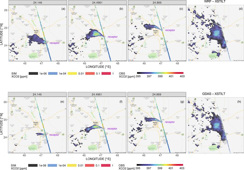
D. Wu et al.: Towards extracting signals of urban CO2 emissions from satellite observations                               4845

   Two main approaches can be considered for atmospheric             adopted to constrain emissions. Approaches to quantify
transport modeling. Eulerian models, in which fixed grid             errors in horizontal wind fields and vertical mixing have
cells are adopted and CO2 concentrations within the grid             been proposed followed by comprehensive error char-
cells are calculated by forward numerical integrations, have         acterizations on atmospheric simulations (Gerbig et al.,
been widely utilized and customized to understand urban              2008; Jeong et al., 2013; Lauvaux et al., 2016; Lin and
emissions and quantify model uncertainties over specific             Gerbig, 2005; Zhao et al., 2009). Recent efforts (e.g.,
metropolitan regions worldwide (Deng et al., 2017; Lauvaux           Lauvaux and Davis, 2014; Ye et al., 2017) have been
et al., 2013; Palmer, 2008; Ye et al., 2017). The Lagrangian         made to rigorously examine the column transport errors.
approach, especially the time-reversed approach in which             The uncertainties in horizontal wind fields and vertical
atmospheric transport is represented by air parcels moving           mixing within X-STILT will be propagated into column
backward in time from the measurement location (“recep-              CO2 space in this study.
tor”), is efficient in locating upwind sources and facilitating
the construction and calculation of the “footprint” (e.g., Lin    3. Determining background XCO2 and characterizing its
et al., 2003) or “source–receptor matrix” (Seibert and Frank,        uncertainties. We define the background value as the
2004) – i.e., the sensitivity of downwind CO2 variations to          CO2 “uncontaminated” by fossil fuel emissions from
upwind fluxes.                                                       the city of interest. As urban emission signals are de-
   In particular, the receptor-oriented Stochastic Time-             fined as the enhancements of XCO2 over the back-
Inverted Lagrangian Transport (STILT) model, a Lagrangian            ground, errors in the background value introduce first-
particle dispersion model (LPDM), has the ability to more re-        order errors into the derived urban XCO2 signal from
alistically resolve the sub-grid scale transport and near-field      total XCO2 , with such errors propagating directly into
influences (Lin et al., 2003). STILT has been used to interpret      fluxes calculated from atmospheric inversions (e.g.,
CO2 observations within the planetary boundary layer (PBL)           Göckede et al., 2010). Consequently, background deter-
(Gerbig et al., 2006; Kim et al., 2013; Lin et al., 2017) and,       mination is another critical task.
in recent years, to analyze column observations, i.e., XCO2          One commonly used method to determine model
(Fischer et al., 2017; Heymann et al., 2017; Macatangay et           boundary conditions of various species in LPDMs is the
al., 2008; Reuter et al., 2014). Among STILT-based XCO2              “trajectory-endpoint” method that establishes the back-
studies, most aim at either natural CO2 sources and sinks like       ground based on CO2 extracted at endpoints of back
wildfire emissions and biospheric fluxes, or anthropogenic           trajectories from modeled regional/global concentration
emissions at regional or state scales. Very few studies have         fields (Lin et al., 2017; Macatangay et al., 2008; Mallia
focused on city-scale FFCO2 using column data and LPDMs.             et al., 2015). The aforementioned studies (adopting the
Moreover, when applying LPDMs to interpret column CO2                trajectory-endpoint method) aim at extracting relatively
data, three key issues have yet to be carefully examined and         large CO2 anomalies (e.g., at a fixed level within the
will be addressed in this paper:                                     PBL or due to large emissions such as of wildfire)
                                                                     from the total measured CO2 . However, for studying
 1. Uncertainty of modeled XCO2 enhancements due to
                                                                     XCO2 that is less variable than near-surface CO2 (Olsen
    model configurations. Very few studies have examined
                                                                     and Randerson, 2004), potential errors in modeled con-
    model uncertainties resulting from model configura-
                                                                     centration fields and atmospheric transport may pose a
    tions, i.e., receptors and particles in LPDMs. A negli-
                                                                     more significant adverse impact on derived urban sig-
    gible amount to ∼ 20 % of the modeled enhancements
                                                                     nals. Other ways of defining the background include ge-
    are reported as the error impact due to the STILT par-
                                                                     ographic definitions (Kort et al., 2012; Schneising et al.,
    ticle number (released from a fixed level), depending
                                                                     2013) and simple statistical estimates (Hakkarainen et
    on adopted particle numbers, examined species, and
                                                                     al., 2016; Silva and Arellano, 2017). These simple sta-
    their components/sources (Zhao et al., 2009; Gerbig
                                                                     tistical methods often neglect atmospheric transport and
    et al., 2003; Mallia et al., 2015). When it comes to
                                                                     may use a less accurate upwind region to select mea-
    representing an atmospheric column using particle en-
                                                                     surements for deriving background values. Lastly, but
    sembles, many studies describe their setups for recep-
                                                                     more importantly, recent column studies (Nassar et al.,
    tors/particles without detailed explanations of why the
                                                                     2017; Fischer et al., 2017) have examined the impact
    setups were chosen or the error impact on modeling
                                                                     of potential errors/biases in the background values on
    XCO2 due to model configurations. Although this error
                                                                     their emission or fluxes estimates. In this work, we in-
    impact may be small, we still perform a set of sensi-
                                                                     troduce a new background determination that combines
    tivity tests to provide more guidance regarding placing
                                                                     OCO-2 observations and the STILT-based atmospheric
    column receptors.
                                                                     transport, and we account for errors in our background
 2. Horizontal and vertical transport error impact on XCO2           estimates.
    simulations. Flux inversions, e.g., Bayesian inversion
    (Rodgers, 2000) involving LPDMs have been widely

www.geosci-model-dev.net/11/4843/2018/                                            Geosci. Model Dev., 11, 4843–4871, 2018
4846                           D. Wu et al.: Towards extracting signals of urban CO2 emissions from satellite observations

Figure 1. A schematic of X-STILT in five steps (represented by the arrows on the right of the figure). Pink and purple dots and arrows
represent the air parcels and overall air flows based on forward-time box runs and backward-time column runs with the wind error component
accounted for. The “rainbow band” (running diagonally through the figure) is an example of one OCO-2 overpass with warmer colors
indicating higher observed XCO2 values. M1 includes modeled-derived biospheric, oceanic XCO2 changes, CO2 boundary conditions, and
the prior CO2 portion from OCO-2. M3 requires an enhanced latitude range based on either backward-time XCO2 enhancements or the
forward-time urban plume.

   In general, we attempt to address the aforementioned is-            2     Data and methodology
sues by extending STILT with column features and com-
prehensive error analyses, referred to as the column-enabled           Before demonstrating the model details, Fig. 1 highlights
STILT, “X-STILT”. We illustrate the model’s application                several X-STILT characteristics, e.g., column transport er-
regarding extracting urban XCO2 signals from OCO-2 re-                 ror quantifications, background XCO2 approximations, and
trievals (Fig. 1) and evaluate model performance via a case            the identification of upwind emitters using backward-time
study focused on Riyadh, Saudi Arabia. Riyadh, which had               runs from column receptors. Our goal is to evaluate the
a population of over 6 million people in 2014 (WUP, 2014),             model by comparing both the latitude-dependent model–
is chosen as the city of interest because of its low cloud in-         data XCO2 urban enhancements (Sect. 3.4) and the over-
terference, limited vegetation coverage, and isolated, barren          all latitude-integrated urban signals within a small latitudi-
location; these factors lead to higher data recovery rates and         nal range (Sect. 3.5). We selected and examined five OCO-
facilitate the background determination. Saudi Arabia has the          2 overpasses during the time period from September 2014
highest CO2 emissions among Middle Eastern countries and               to December 2016, based on four stringent criteria (Ap-
ranked eighth globally in 2016 (Boden et al., 2017; BP, 2017;          pendix A).
UNFCCC, 2017). We examine several satellite overpasses
and focus on a small spatial domain adjacent to Riyadh for             2.1    STILT-based approach for XCO2 simulation
each overpass.                                                                (“X-STILT”)

                                                                       The OCO-2 column averaging kernel is the product of nor-
                                                                       malized averaging kernel (AKnorm ) and the pressure weigh-
                                                                       ing (PW) function and represents the sensitivity of the change

Geosci. Model Dev., 11, 4843–4871, 2018                                                   www.geosci-model-dev.net/11/4843/2018/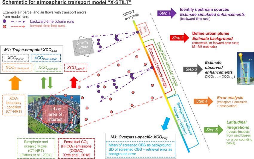
D. Wu et al.: Towards extracting signals of urban CO2 emissions from satellite observations                                 4847

in retrieved XCO2 due to the CO2 anomaly at each retrieved
grid. Column AKnorm peaks near the surface and exhibits val-
ues near unity throughout most of the troposphere (Boesch          XCO2.sim.ak = XCO2.sim.ff + XCO2.sim.bio + XCO2.sim.ocean
et al., 2011). Lower AKnorm values are mainly found aloft,                     + XCO2.sim.bound + XCO2.prior
which means that more information is required in the a pri-                     = XCO2.sim.ff + XCO2.bg .                     (2)
ori CO2 profiles (CO2,prior ; Fig. 2a). For direct comparisons
against OCO-2 retrieved XCO2 , CO2 anomalies at model              Given our focus, we defined the background value as the
grids should be properly weighted using the satellite’s col-       XCO2 portion not “contaminated” by urban emissions. Thus,
umn averaging kernels (Basu et al., 2013; Lin et al., 2004).       XCO2.sim.ak is the sum of the XCO2 enhancement due to
Thus, the final AK-weighted simulated XCO2 (XCO2.sim.ak )          FFCO2 (XCO2.sim.ff ) and the estimated background value
are weighted between model-derived CO2 profiles and OCO-           (XCO2.bg ). Estimates of XCO2 anomalies are further ex-
2 a priori profiles (O’Dell et al., 2012):                         plained in Sect. 2.1.2, and four ways to estimate background
                                                                   values (XCO2.bg ) are proposed in Sect. 2.3.
                nlevel
                 X
XCO2.sim.ak =            AKnorm,n PWn CO2.sim,n                    2.1.1   X-STILT setup (“column receptors”)
                n=1

                + 1 − AKnorm,n PWn CO2.prior,n .            (1)    The linkage between the observed XCO2 concentration from
                                                                   a given OCO-2 sounding and upwind CO2 sources and sinks
In the abovementioned equation, n stands for the combined          is determined by atmospheric transport. We adopt the STILT
vertical levels of STILT plus OCO-2. Specifically, we re-          model to describe this connection. Fictitious particles, rep-
placed OCO-2 levels with denser model release levels for the       resenting air parcels, are released from a “receptor” (loca-
lower part of the troposphere (red circles from the surface        tion of interest) and are dispersed backward in time. The
in Fig. 2), while we kept OCO-2 levels for upper part of the       Lagrangian air parcels within STILT are transported along
troposphere (blue circles in Fig. 2). To reduce computational      with the mean wind (u), turbulent wind component (u0 ), and
cost, the air column is only simulated up to the maximum           other meteorological variables, which are derived from Eu-
release height (MAXAGL, in meters above ground level –             lerian meteorological fields. In this study, we used meteoro-
m a.g.l.; Fig. 2).                                                 logical fields simulated by the Weather Research and Fore-
   Interpolations are further needed to resolve the mismatch       casting (WRF; Skamarock and Klemp, 2008) model and the
between prescribed OCO-2 retrieval grids and model lev-            0.5◦ × 0.5◦ Global Data Assimilation System (GDAS; Rolph
els for the lower part of the troposphere. Our intention is        et al., 2017; Stein et al., 2015). Hourly WRF fields contain 51
to preserve the finer modeled CO2 variations by perform-           vertical levels with boundary conditions from 6 h 0.5◦ × 0.5◦
ing interpolations of satellite profiles from retrieval grids to   NCEP FNL (final) operational global analysis data (Ye et al.,
model levels. Vertical profiles of AKnorm , PW and CO2,prior       2017) and are customized and utilized for the first two of the
are treated as continuous functions and interpolated linearly      five total overpasses over Riyadh. We note that the primary
to model grids (red circles in Fig. 2). Note that the initial      focus is on assessing the resulting errors given the choice of
OCO-2 PW functions have a steady value of ∼ 0.052 (except          a particular wind field (i.e., GDAS 0.5◦ ), rather than on car-
for the very bottom and top levels; black dots in Fig. 2b),        rying out detailed analyses of differences between WRF and
which results from constant pressure spacings (dp_oco2) be-        GDAS.
tween two adjacent OCO-2 levels. However, X-STILT levels              To represent the air arriving at the atmospheric column of
are much denser with smaller pressure spacings (dp_stilt) or       each OCO-2 sounding, we release air parcels from multiple
less air mass between their two adjacent levels. Therefore,        vertical levels, “column receptors” (Fig. 3e), using the same
the linearly interpolated PW (red circles in Fig. 2b) needs ad-    lat/long coordinates as the satellite sounding at the same time
ditional scaling via a set of “scaling factors” representing the   and allow those parcels to disperse backward for 72 h (see
ratios of pressure spacings in STILT versus OCO-2 retrieval        Appendix D2 for model impact from backward durations).
(dp_stilt/dp_oco2), to arrive at the correct PW for each finer     About 10–20 satellite soundings are selected for simulations
model grid (orange circles in Fig. 2b).                            over every 0.5◦ latitude with data filtering using the crite-
   Equation (1) can further be rewritten as Eq. (2), as the sim-   ria explained in Sect. 2.2. Sensitivity tests are conducted re-
ulated CO2 profile in Eq. (1) is comprised of a CO2 boundary       garding different configurations – the maximum release level
condition plus CO2 anomalies due to sources/sinks (FFCO2 ,         (MAXAGL), the vertical spacing of release levels (dh), and
biospheric, and oceanic fluxes):                                   the particle number per level (dpar) – when placing column
                                                                   receptors (Sect. 2.5).

                                                                   2.1.2   Modeling XCO2 anomalies

                                                                   Air parcels traveling back in time provide valuable informa-
                                                                   tion about how upwind sources and sinks impact the air ar-

www.geosci-model-dev.net/11/4843/2018/                                               Geosci. Model Dev., 11, 4843–4871, 2018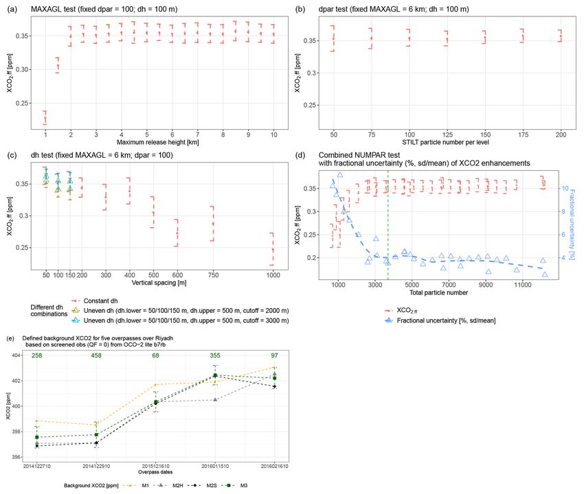
4848                            D. Wu et al.: Towards extracting signals of urban CO2 emissions from satellite observations

Figure 2. Demonstrations of interpolations on the (a) normalized averaging kernel (AKnorm ) profile, (b) pressure weighing (PW) function,
and (c) the CO2 boundary conditions (derived from CarbonTracker – CT-NRT) and OCO-2 a priori profile, given one sounding (with the same
lat/long coordinates as column receptors). The red and blue shading denotes the X-STILT release levels from the surface up to MAXAGL
and upper OCO-2 levels, respectively.

riving at a receptor. However, since particles within the en-          et al. (2018) for additional details pertaining to the formula-
semble are subject to stochastic motion, the surface fluxes            tion of f .
observed by any single particle caries limited information.               We introduce the weighted column footprint fw that de-
The influence of upstream surface fluxes on a receptor is              scribes the sensitivity of changes in column concentration
given by summing the sensitivities of all particles in the en-         due to potential upstream sources/sinks and incorporates
semble over a surface grid f (x, y, t), which is referred to           satellite profiles. The formulation of fw is similar to Eq. (3)
as the “footprint” (Lin et al., 2003; Fasoli et al., 2018) or          but scales the sensitivity with AKnorm (n, r) and PW (n, r):
the “source–receptor matrix” (Seibert and Frank, 2004). For-
                                                                                                            mair         1
mally, the sensitivity of the receptor located at xr at time tr

                                                                       fw xn,r , tn,r |xi , yj , tm =
to surface fluxes originating from xi , yj is given by summing                                          hρ xi , yj , tm Ntot
1tp,i,j,z≤h , the time spent by particle p over grid position ij           Ntot
                                                                           X
within the surface layer of height h for each discrete time step                  1tp,i,j,z≤h AKnorm (n, r) PW (n, r) ,              (4)
m:                                                                         p=1

                                                                       where xn,r , tn,r denotes a column receptor. Multiplying fw

f xr , tr |xi , yj , tm
                             Ntot                                      by gridded flux estimates yields a change in CO2 at the down-
            mair         1 X                                           wind column receptor. Thus, surface fluxes F xi , yj , tm
    =                            1tp,i,j,z≤h ,               (3)
        hρ xi , yj , tm Ntot p=1                                       cause a change in column integrated mole fraction 1XCO2
                                                                       as follows:
where Ntot is the total number of particles in the ensemble,
mair is the molar mass of dry air, and ρ is the average air            1XCO2 xn,r , tn,r |xi , yj , tm
density below h. The dilution of surface fluxes to half of the
                                                                           = F xi , yj , tm fw xr , tr |xi , yj , tm .            (5)
PBL height h = 0.5zpbl is often used. In general, f increases
if particles travel at heights z ≤ h and if h is low, concentrat-      For this study, modeled XCO2 enhancements due to FFCO2
ing surface fluxes within a shallower atmospheric column.              emissions are derived from the convolution of spatially vary-
   To reduce grid noise caused by the aggregation of a finite          ing fw and ODIAC emissions (Sect. 2.4.1). Also, we account
number of dispersed particles, a kernel density estimator is           for modeled uncertainties that include errors in prior FFCO2
used to variably smooth f as a function of elapsed time and            emissions (Sect. 2.4.1), receptor configurations (Sect. 2.5),
particle location uncertainty. The reader is referred to Fasoli        and atmospheric transport (Sect. 2.6).

Geosci. Model Dev., 11, 4843–4871, 2018                                                    www.geosci-model-dev.net/11/4843/2018/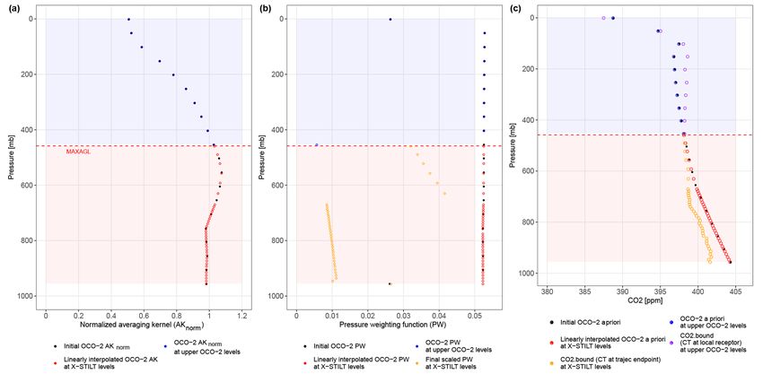
D. Wu et al.: Towards extracting signals of urban CO2 emissions from satellite observations 4849
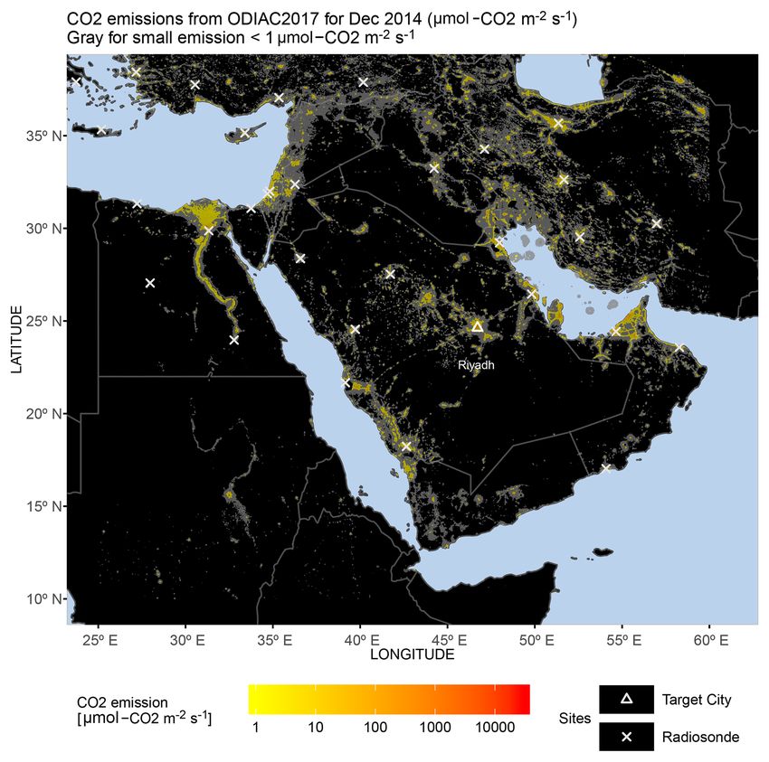
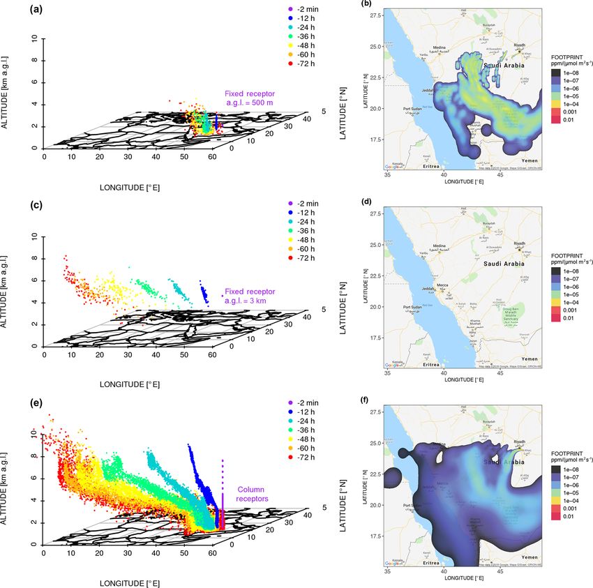
Figure 3. A 3-D scatterplot of STILT ensembles that are initially released from a fixed receptor of 500 m(a), 3 km(c), and column receptors(e)
for Riyadh at 10:00 UTC on 29 December 2014. The different colors represent the number of minutes/hours backwards (−2 min, −12, −24,
−36, −48, −60, and −72 h) for each trajectory. Column receptors (e) are placed every 100 m within 3 km and every 500 m from 3 to 6 km. (b,
d, f) Modeled fixed footprints versus column footprints are plotted using a blue to red gradient. Column footprints are weighted by pressure
weighing functions. Only footprint values > 1E-8 ppm / (µmol m−2 s−1 ) are displayed.
2.2 OCO-2 retrieved XCO2 and data preprocessing 2 lite files (version 7R; OCO-2 Science Team/Michael Gun-
son, Annmarie Eldering, 2015). The impacts of different ver-
sions of the OCO-2 datasets on our results are briefly dis-
The OCO-2 algorithm for retrieving XCO2 from radiances
cussed in Sect. 5. Satellite measurements over Riyadh were
employs an optimal estimation approach (Rodgers, 2000) in-
carried out in “land nadir” and “glint” modes. Soundings
volving a forward model, an inverse model, and prior in-
with quality flags equal zero (QF = 0) were selected; this
formation regarding the vertical CO2 profiles (O’Dell et al.,
implied that the selected observations had passed the cloud
2012). We used the bias-corrected XCO2 values from OCO-
www.geosci-model-dev.net/11/4843/2018/ Geosci. Model Dev., 11, 4843–4871, 20184850 D. Wu et al.: Towards extracting signals of urban CO2 emissions from satellite observations
and aerosol screening (with removal of albedo > 0.4) and fluxes, oceanic fluxes, and OCO-2 prior profiles (M1 in Fig. 1
that their retrievals had converged (Mandrake et al., 2013; and Eq. 2). Specific for modeling CO2 boundary conditions,
Patra et al., 2017). For smoothing noisy observations, we CO2 values for upper levels, above MAXAGL, are estimated
binned the screened XCO2 data according to the lat/long co- based on CT CO2 at those OCO-2 pressure levels (purple cir-
ordinates of model receptors (that served as the midpoints cles in Fig. 2c). Averaged CO2 values from the global model
of each bin) and calculated the mean and standard devia- extracted at trajectory endpoints are used for boundary condi-
tion of screened measurements within each bin. Next, back- tions at model release levels (orange circles in Fig. 2c). Then,
ground values were defined (Sect. 2.3) and subtracted from modeled boundary conditions at vertical levels are weighted
the bin-averaged observed XCO2 to estimate the increase in accordingly via OCO-2’s column averaging kernel (red and
observed XCO2 (step 3 in Fig. 1). The impacts of different blue circles in Fig. 2c). Model trajectories are properly sub-
bin-widths on the bin-averaged observed signals are shown in setted according to the boundary of the footprint domain (i.e.,
Appendix E1. Total observed errors contain the spatial and 20◦ × 20◦ ) used for simulating the XCO2 anomalies.
natural variation of observed XCO2 in each bin, the back- We note that for the trajectory-endpoint method, poten-
ground uncertainties (Sect. 2.3.3), and the retrieval errors tial uncertainties in transport may strongly influence the dis-
provided by lite files. Retrieval error variances per sound- tribution of Lagrangian parcels as backward duration time
ing are then averaged within each observed bin to obtain the increases and may lead to potential spatial mismatch of the
bin-averaged retrieval error variances. background region. Furthermore, potential biases and the rel-
atively coarse resolution of the adopted global product may
2.3 Estimates of background XCO2 add inaccuracies to CO2 values at trajectory-endpoints.
Definitions of “background” vary among studies with dif- 2.3.2 Statistical method (M2)
ferent applications. Here, we define the background values
as atmospheric XCO2 that is not “contaminated” by the ur- Hakkarainen et al. (2016) (referred to as M2H) extracted
ban emissions around our study site. The determination of local XCO2 anomalies from the daily median of screened,
background XCO2 is crucial, as it can significantly affect the measured XCO2 within a relatively broad region (0–60◦ N,
magnitude of inferred observed anthropogenic signals. If the 15◦ W–60◦ E over the Middle East; Fig. S7 in the Supple-
background is underestimated, then the detected signal may ment). Their detected anomalies vary from 1 to 2 ppm over
be overestimated, and vice versa. In this study, we seek to de- 0.5◦ × 0.5◦ grid cells near Riyadh. Silva and Arellano (2017)
velop the best-estimated background values given five tracks, (referred to as M2S) used measurements within a 4◦ × 4◦
where three methods are proposed and investigated as fol- combustion region centered around “urban and dense settle-
lows: ments” inferred from the anthropogenic biomes dataset (“an-
thromes”; Ellis and Ramankutty, 2008). Then, they derived
– M1. a “trajectory-endpoint” method is investigated by the background as the mean minus 1 standard deviation of
assigning CO2 values extracted from global models to the available observations within their studied urban extents.
trajectory endpoints including simulating biospheric, While both statistical methods are highly efficient in esti-
oceanic, and prior components (Sect. 2.3.1); mating background values, they can be limited to certain ap-
– M2. statistical methods estimate the background values plications. For instance, M2H may be not suitable for deter-
solely from XCO2 observations based on two previous mining background values when zooming into specific cities.
studies (Sect. 2.3.2); Measurements within their broad spatial domain are lumped
together, regardless of their locations (whether over rural
– M3. an “overpass-specific” background that requires a or urban areas) and atmospheric transport. Silva and Arel-
model-defined urban plume and measurements outside lano (2017) have also pointed out that their defined 4◦ × 4◦
the plume is examined (Sect. 2.3.3). combustion region is suitable for studying the “bulk” charac-
teristics and may be too coarse for studying urban emissions.
We compare the aforementioned three methods (Sect. 3.3) Furthermore, the Gaussian statistics assumed in M2S may be
and investigate the background impact on model–data com- less applicable when multiple observed peaks are merged due
parisons and emission estimates (Sect. 4.2). We choose the to close proximity between clusters of multiple cities. There-
M3-based background for the following analysis as it is fore, without incorporating much atmospheric transport in-
specifically designed for examining a particular city and spe- formation, it may be difficult for either statistical method to
cific overpasses downwind of the city. locate the exact XCO2 peak elevated by target city or back-
ground region. These difficulties motivate us to introduce a
2.3.1 Trajectory-endpoint method (M1)
new approach in the next subsection.
Modeled background XCO2 comprises a simulated boundary
condition confined by 4-D CO2 fields from a global model
(CT-NRT; see Sect. 2.4.2) and contributions from biospheric
Geosci. Model Dev., 11, 4843–4871, 2018 www.geosci-model-dev.net/11/4843/2018/D. Wu et al.: Towards extracting signals of urban CO2 emissions from satellite observations 4851
(Thomas Nehrkorn, personal communication, 2017) to track
air parcels over a city and the transport of the urban plume.
Specifically, the model continuously releases air parcels over
a 30 min window from a 0.4◦ × 0.4◦ box around the city cen-
ter, with multiple 30 min releases of 1000-particle ensem-
bles over the 10 h before the satellite overpass hour (00:00–
10:00 UTC). An urban plume can then be derived from the
parcels’ distribution during the ∼ 3 min OCO-2 passing win-
dow (purple dots in Fig. 5a). Note that air parcels are tracked
forward in time for 12 h, allowing for equal contributions
from parcels that were initially released from different time
intervals (every 30 min) into the defined urban plume. We
are aware of potential model errors and their adverse impacts
on the defined urban plume. Therefore, a wind error compo-
nent (Sect. 2.6) is also added in the forward run to broaden
the polluted range (solid black line in Fig. 5a). Next, 2-D
kernel density estimation (Venables and Ripley, 2002) is ap-
plied to determine the boundary of the city plume based on
the air parcels’ distributions. We normalized the 2-D kernel
density by its maximum value and sketched the boundary of
the city plume based on a threshold kernel density value of
Figure 4. Monthly ODIAC emissions (yellow to orange) in log- 0.05, which is sufficient to include most air parcels. No dra-
scale at 1 km×1 km grid spacing for December 2014. White crosses matic change in the shape/size of the resultant urban plume
and the triangle denote the radiosonde networks used to provide was found when testing other thresholds < 0.05. The urban-
the wind error statistics and our study site of Riyadh, respectively. influenced latitude range is defined as the intersection of the
Small emissions (< 1 µmol m−2 s−1 ) are shaded in gray. urban plume and the OCO-2 overpass (Fig. 5a). Overall, the
urban-influenced latitudinal band represented by 5 % of the
maximum kernel density covers the area from 23.5 to 26◦ N,
2.3.3 Overpass-specific background (M3) given multiple overpasses for Riyadh (Fig. S2). The back-
ground latitudinal range unaffected by Riyadh’s urban plume
A few space-based studies have defined the background val- for the estimating background then extends ∼ 100 km from
ues as the averaged observed XCO2 values over a “clean” up- the northernmost and/or southernmost limits of the derived
wind region. For instance, Kort et al. (2012) and Schneising urban plume (Fig. 5b). We neglect observations with lati-
et al. (2013) defined the “clean” region based on geographic tudes > 26 and < 23◦ N, because these retrievals are too scat-
information (e.g., rural area to the north of the Los Angeles tered (black triangles in Fig. 5b) and may indicate a second
basin). Although OCO-2 has relatively narrow swaths, trans- peak during other overpasses. If the near-field wind vectors
port models can be used to differentiate the enhanced versus point more toward the north, screened measurements over the
background portions along an overpass. For example, Janar- southern background latitudinal range are utilized, and vice
danan et al. (2016) calculated background XCO2 as the av- versa. Eventually, the background value is calculated as the
eraged GOSAT observations among grid cells with modeled mean value of the screened observations over the background
anthropogenic signals < 0.1 ppm. This 0.1 ppm threshold is region (dashed green line in Fig. 5b). Two error sources are
determined from the average simulated fossil fuel abundance incorporated into the background error: the measured (stan-
over desert areas worldwide using the FLEXible PARTicle dard deviation, SD) and the retrieval errors of background
dispersion model (FLEXPART; Stohl et al., 2005), a model observations.
similar to STILT in that both are time-reversed LPDMs. In addition to random errors accounted for by the inclusion
Nassar et al. (2017) derived the overpass-dependent back- of the aforementioned wind error component and broadening
ground and its uncertainty based on the averaged OCO-2 ob- of the city plume, potential large biases in near-field wind di-
servations within four different tested background latitudinal rection may lead to a mismatch in the modeled and observed
ranges. background regions and may bring relatively higher XCO2
We present an alternative method using a forward-time values into background XCO2 . However, we do not explic-
run from an urban box to reveal the urban influence on itly account for the potential impact of near-field wind biases
satellite soundings, which are more straightforward and ef- on the forward-trajectories defined urban plume due to the
ficient than relying solely on backward-time runs. Fictitious following considerations. Firstly, we attempted to propagate
particles are released from a box around the city center a near-field wind bias into the modeled plume by rotating
(pink dots in Fig. 1) as a feature implemented with STILT the forward trajectories, whereas the robustness of this near-
www.geosci-model-dev.net/11/4843/2018/ Geosci. Model Dev., 11, 4843–4871, 20184852 D. Wu et al.: Towards extracting signals of urban CO2 emissions from satellite observations Figure 5. Demonstration of the overpass-specific background using the 29 December 2014 overpass for Riyadh as an example. (a) Forward particle distributions with random transport error included (blue and purple dots) and their derived normalized kernel density (solid purple contours) during the OCO-2 overpass time (∼ 3 mins) with observed XCO2 (blue to red dots). Urban plumes are defined based on 5 % of the max 2-D kernel density estimated from parcels’ distributions without (gray dashed line) and with (black solid line) transport errors. (b) Latitude-series of observed XCO2 with the demonstration of background estimates. Smooth splines (solid blue lines) are drawn to visually reveal the variation of observed XCO2 over the background latitudinal band. The background uncertainty (green shaded area) includes both the spatial uncertainty and the retrieval uncertainty of observations over the background latitude range. field bias can be affected by the rare wind measurements near less accurate background range and could potentially bring Riyadh (further explained in Sect. 2.6.1). Secondly, the back- elevated XCO2 into the background, the background uncer- ground latitude range defined by M3 with the broadening ef- tainty implicitly contains information about the spatial vari- fect (blue curves in Fig. 5b) generally matches well with that ation in background measurements (green shaded region in observed from OCO-2 for most overpasses, which implies Fig. 5b). Furthermore, the M3-derived background is gener- that the overall wind bias around our study site is not signif- ally the mean value of hundreds of background observations icant. Lastly, even if the potential wind bias may result in a (numbers of observations shown in Fig. 6e), which may not Geosci. Model Dev., 11, 4843–4871, 2018 www.geosci-model-dev.net/11/4843/2018/
D. Wu et al.: Towards extracting signals of urban CO2 emissions from satellite observations                                4853

be greatly affected by a few potential urban-enhanced mea-      2.4.2    Natural fluxes (CarbonTracker)
surements.
                                                                The trajectory-endpoint method (M1 in Sect. 2.3.1) requires
2.4     Sources of information for CO2 fluxes
                                                                the oceanic and terrestrial biospheric fluxes from the 3 h
2.4.1    Fossil fuel emission (ODIAC) and prior emission        product – CarbonTracker Near-Real Time (CT-NRT.v2016
         uncertainties                                          and CT-NRT.v2017, http://carbontracker.noaa.gov, last ac-
                                                                cess: 27 July 2017). CT-NRT, an extension of the standard
To calculate modeled XCO2 enhancements, we used the lat-        CarbonTracker (Peters et al., 2007), is designed for the OCO-
est (2017) version of the Open-Data Inventory for Anthro-       2 program and uses different prior flux models and “real-
pogenic Carbon dioxide (ODIAC2017 dataset, Oda et al.,          time” ERA-Interim reanalysis in its transport model than
2018; Oda and Maksyutov, 2011, 2015) with monthly fossil        regular CT, which allows for more timely model results. To
fuel CO2 emissions at a 1 × 1 km resolution (Fig. 4). ODIAC     calculate oceanic and biospheric XCO2 changes, we multi-
starts with annual national emission estimates, separated by    plied these natural fluxes by the column weighted footprint
fuel type, from the Carbon Dioxide Information Analysis         according to Eq. (5). Although wildfire emissions can greatly
Center (CDIAC, Andres et al., 2011), which are then re-         modify atmospheric XCO2 (e.g., Heymann et al., 2017), we
categorized into specific ODIAC emission categories on a        expected relatively small XCO2 contributions from wild-
monthly basis, i.e., point source, non-point source, cement     fire; hence, we excluded wildfire-elevated XCO2 estimations,
production, international aviation, and marine bunker (Oda et   considering the periods studied (wintertime overpasses) and
al., 2018). Because CDIAC only covers the years up to 2013,     the study region (the Middle East). Note that the horizontal
ODIAC extrapolates emissions in 2013 for emissions in 2014      grid spacing of oceanic and biospheric fluxes provided by
and 2015 based on BP (i.e., the British Petroleum Company)      CT-NRT is 1◦ × 1◦ ; while the grid spacing of the CT-NRT
global fuel statistical data (BP, 2017). ODIAC also estimates   4-D CO2 fields previously mentioned in Sect. 2.3.1 is 2◦ ×3◦
point source emissions according to a global power plants       over the Middle East.
database – the Carbon Monitoring and Action (CARMA)
database (Wheeler and Ummel, 2008), and collects and dis-       2.5     Sensitivity analyses for X-STILT column receptors
tributes non-point source emissions using an advanced night-
time lights dataset from the Defense Meteorological Satellite
                                                                The goal of carrying out sensitivity tests is to understand
Program Operational Line Scanner (DMSP/OLS). The use
                                                                any systematic/random errors of STILT simulations caused
of the nightlight dataset allows ODIAC to characterize the
                                                                by receptor configurations. Under the premise of limited
spatial patterns of the anthropogenic sources such as point
                                                                computational resources, proper column receptors are set
sources, line sources, and diffuse sources.
                                                                up with allowable random errors. The total number of par-
   To estimate emission uncertainties, we followed a method
                                                                ticles (NUMPAR) released from column receptors are de-
similar to those reported in Oda et al. (2015) and Fischer
                                                                composed into three parameters: the maximum release level
et al. (2017). Three emission inventories derived from dif-
                                                                (MAXAGL), the vertical spacing of release levels (dh), and
ferent methods are intercompared: ODIAC, the Fossil Fuel
                                                                the particle number per level (dpar).
Data Assimilation System (FFDASv2; Asefi-Najafabad et
                                                                   Instead of regenerating model trajectories (Jeong et al.,
al., 2014; Rayner et al., 2010) and the Emission Database for
                                                                2013; Mallia et al., 2015), we adopted the bootstrap method
Global Atmospheric Research (EDGARv4.2; http://edgar.
                                                                to resample model ensembles. The bootstrap approach helps
jrc.ec.europa.eu, last access: 10 December 2013; Janssens-
                                                                construct hypothesis tests and infer error statistics (Efron and
Maenhout et al., 2017). To resolve different spatial grid
                                                                Tibshirani, 1986). The initial sample size before the boot-
spacing among the three inventories, we aggregated ODIAC
                                                                strap should be large enough to ensure the performance of
emissions from 1 km to 0.1◦ grid cells. The fractional un-
                                                                the bootstrap method and its related statistics. Thus, a “base
certainty for gridded emissions is characterized by the emis-
                                                                run” of trajectories starting from the surface to 10 km with a
sion spread (1σ , among three inventories) and mean values
                                                                vertical spacing of 25 m and 200 particles per level is gener-
(µ) of estimated emissions for each grid cell within a given
                                                                ated and stored. For testing each parameter (MAXAGL, dh,
region (10–40◦ N, 25–60◦ E; Fig. S3). In general, fractional
                                                                or dpar), we fixed the other two parameters and randomly se-
uncertainties in gridded emissions mostly range from 60 % to
                                                                lected/resampled model particles from the base run 100 times
130 % (Fig. S3) around Riyadh. Ultimately, these fractional
                                                                allowing for repetitions. A hundred urban enhancements are
emission uncertainties and ODIAC emissions are convolved
                                                                calculated from 100 new sets of trajectories for each test. Ba-
with X-STILT’s weighted column footprints to provide the
                                                                sic statistics – i.e., mean values and standard deviations (or
XCO2 uncertainties due to prior emission uncertainties.
                                                                fractional uncertainty, i.e., SD/mean) among these 100 en-
                                                                hancements – are used to infer systematic and random uncer-
                                                                tainties in each test, respectively (the results are displayed in
                                                                Sect. 3.1).

www.geosci-model-dev.net/11/4843/2018/                                            Geosci. Model Dev., 11, 4843–4871, 2018
4854 D. Wu et al.: Towards extracting signals of urban CO2 emissions from satellite observations
2.6 X-STILT column transport errors tion of modeled AK-weighted XCO2 in Eq. (1), the weighted
column transport error follows Eq. (6):
Uncertainty in atmospheric transport modeling has been
identified to significantly affect emission constraints (Cui et nlevel
X
σε2 (XCO2.sim.ak ) = wn2 σε2 CO2.sim.ak,n
al., 2017; Lauvaux et al., 2016; Stephens et al., 2007). Here
n=1
we quantify uncertainties in modeled XCO2 due to transport X
errors caused by uncertainties in both horizontal wind fields +2 wn wm covε CO2.sim.ak,n , CO2.sim.ak,m , (6)
1≤nD. Wu et al.: Towards extracting signals of urban CO2 emissions from satellite observations 4855
print magnitude and the its spatial distribution via differ- In addition, we conducted two experiments using constant
ent horizontal advections at each altitude. Although column- and uneven vertical spacings with a fixed MAXAGL of 6 km
integrated measurements may be less sensitive to the verti- and a dpar of 100. Vertical spacing in the constant dh exper-
cal distribution of air particles than in situ measurements, iment ranges from 50 m to 1 km. Mean enhancements gen-
vertical transport errors can nonetheless have some impacts erally decrease as the vertical spacing increases (red dots in
on column simulations, due to wind shear and its interac- Fig. 6c), likely because fewer release levels are insufficient to
tion with vertical redistribution of air parcels (Lauvaux and represent air parcels in a column and their interactions with
Davis, 2014). Comprehensive quantifications of the vertical surface emissions, especially under strong wind shear. We
transport errors in a column sense are performed in Lauvaux further performed two cases with uneven vertical spacing be-
and Davis (2014) using an ensemble of surface and plane- low and above a “cutoff level”. Both cases tested three differ-
tary boundary layer (SBL-PBL) parameterizations involving ent lower spacings (of 50, 100, or 150 m) with a fixed upper
a regional inverse modeling framework. spacing of 500 m. The two cases differ only in their cutoff
Here, we made use of the stochastic nature of STILT levels (2 or 3 km). The comparison of the uneven dh with the
and propagated typical PBL height errors in the model. constant dh experiment shows that their XCO2 enhancement
Changes in STILT-modeled mixed layer height modify the results are fairly similar; this suggests that the lower spac-
vertical profiles of turbulent statistics that directly control the ing below the cutoff level matters most with respect to the
stochastic motions of the Lagrangian air parcels (Lin et al., model results, because most anthropogenic XCO2 enhance-
2003). Thus, we obtained different air parcel trajectories with ments are confined within the PBL. Furthermore, results for
rescaled PBL heights. The resultant vertical transport error the uneven dh case with the cutoff level of 3 km (blue trian-
in XCO2 space is calculated as the root-mean-squared errors gles in Fig. 6c) are more closed to the “truth” implied by the
(RMSEs) between two sets of XCO2 enhancements among constant dh case (red dots in Fig. 6c). To be safe, column re-
different receptors for each overpass. Due to this calcula- ceptors are placed from 0 to 3 km with a spacing of 100 m
tion, vertical transport errors are only provided at the over- and from 3 to 6 km with a spacing of 500 m. See Appendix D
pass level (results in Sect. 3.5). Gerbig et al. (2008) reported for the derivation of the cutoff level.
typical relative PBL errors in the range of ±20 %. Thus, we To summarize, the fractional uncertainties in modeled
rescaled the PBL heights higher and lower by 20 % and eval- XCO2 enhancements reduce rapidly as total particle number
uated the scaling’s impact on XCO2 enhancements. Due to increases (blue triangles in Fig. 6d). Our choice of column
our focus on the urban emissions and potential small XCO2 receptors and particle numbers has no noticeable bias and a
enhancement contributions beyond 1 day backward in time, fractional uncertainty of ∼ 4 % per simulation (dashed green
we only rescaled the PBL within the first 24 h of transport line in Fig. 6d). Overall changes in X-STILT column recep-
before arrival of the air parcels at the column receptors. tors have a fairly small impact on the modeled anthropogenic
signals, which is consistent with the finding (for biospheric
signals) in Reuter et al. (2014).
3 Results
3.2 X-STILT column footprints and upwind emission
3.1 X-STILT sensitivity tests with column receptors
contributions
Figure 6 shows test results from a sounding on 29 Decem-
ber 2014 around Riyadh. In general, urban enhancements Upstream source regions and their contributions to the down-
increase as MAXAGL increases from 1 to 2 km and then wind air column can be identified as the “footprint” us-
stabilize (Fig. 6a). When MAXAGL is small (< 2 km), the ing backward-time simulations. Here we illustrate the dif-
model fails to fully capture the CO2 enhancements within ferences in parcel distributions and footprint patterns de-
the mixing height and causes underestimations of the ele- rived from 500 m, 3 km, and multiple levels, for one sound-
vated XCO2 . Random errors reflect the stochastic nature of ing at 24.4961◦ N on 29 December 2014 (when southwestern
the model particles leading to small fluctuations in parcel dis- winds dominated). Air parcels released at 500 m are asso-
tributions and resultant signals. In this experiment, dpar and ciated with large footprints in the adjacent area of Riyadh
dh are fixed to 100 particles and 100 m. For testing parti- (Fig. 3b). While parcels released from a higher level of
cle number per level (dpar), MAXAGL is set to 6 km (well 3 km travel backwards much faster to upwind regions, most
above the top of the PBL; see Appendix D for the choice of parcels hardly get entrained back into the PBL (Fig. 3c) and
6 km). No obvious bias is associated with mean XCO2 en- make minimal contact with the surface (implied from the
hancements. The random error reduces as particle numbers zero footprint values in Fig. 3d). When air parcels are re-
increases (error bars in Fig. 6b). We ended up placing 100 leased from multiple levels, the column footprints (Fig. 3f)
particles for each level, as random errors do not change dra- cover a broader spatial domain with relatively smaller val-
matically from 100 to 200 particles. ues than footprints derived from 500 m (Fig. 3b). Thus Fig. 3
highlights the difference in upwind influences from a PBL-
based, tower-like measurement versus a column-integrated
www.geosci-model-dev.net/11/4843/2018/ Geosci. Model Dev., 11, 4843–4871, 20184856 D. Wu et al.: Towards extracting signals of urban CO2 emissions from satellite observations
Figure 6. Results of sensitivity tests for one sounding (a–d) and background comparisons for five tracks (e) over Riyadh. The random error
for each simulation is indicated using dashed red error bars (a–d); potential biases are shown as the trend of the mean XCO2 enhancements
(red dots; a–d) derived from 100 bootstraps. (c) Vertical spacing tests include several tests with constant dh (red dots and error bars) and two
tests with uneven dh above/below the cutoff level. The two uneven dh tests both use three different lower dh (50, 100, and 150 m) and a fixed
upper dh of 500 m, but with two different cutoff levels, i.e., 2 km (yellow-green triangles and error bars) and 3 km (blue triangles and error
bars). (d) A summary plot of the mean and SD of the XCO2 enhancements (red dots and dashed red error bars) and fractional uncertainties
(%; blue triangles and dashed line) as functions of total particle number (NUMPAR). The green dashed vertical line denotes the configuration
used in this study. (e) Background comparisons using different methods (M1, M2H, M2S, and M3) for five tracks. The number of screened
observations used for M3 background is noted in dark green. M3 background errors (including spatial variation and retrieval errors over the
background region) are indicated as dashed green error bars.
measurement. As expected, surface influence arriving at an 3.3 Comparisons between methods used to calculate
air column can be 1 or a few orders of magnitude smaller background XCO2
than that arriving at a given location. Consequently, CO2
changes within the PBL are expected to be larger than col-
umn changes. As Silva and Arellano (2017) have pointed out, their 4◦ × 4◦
urban extent may be too coarse for studying urban emissions.
Thus, we adopted their statistical method (µ − σ ) and used
a smaller 2◦ × 2◦ domain instead for computing the back-
ground of M2S. M2S and M3 calculate background values
Geosci. Model Dev., 11, 4843–4871, 2018 www.geosci-model-dev.net/11/4843/2018/D. Wu et al.: Towards extracting signals of urban CO2 emissions from satellite observations 4857
from local observations. Therefore, M2S may agree better observations for the 29 December 2014 overpass (Fig. 8). Al-
with M3 in their derived background regarding both the tem- though XCO2 contributions using GDAS and WRF can differ
poral variations and their magnitudes (black diamonds and in their spatial distributions for some receptors (Fig. 7b ver-
green squares in Fig. 6e). The M1 modeled background dif- sus Fig. 7f), the overall XCO2 contributions integrated from
fers significantly from the other three and exhibits positive all receptors along the overpass (Fig. 7d versus Fig. 7h) share
biases spanning roughly from 0.5 to 1.5 ppm (orange dots in fairly similar spatial distributions and magnitudes and indi-
Fig. 6e). Reasons for this large bias may be the accumulated cate large contributions due to urban emissions from Riyadh
transport errors as the backward duration increases in combi- and small contributions from regions to the south of Riyadh.
nation with potential errors in the global concentration fields, Regarding the shape of latitude-dependent XCO2 enhance-
due to its coarse resolution. ments, large enhancements inferred from bin-averaged ob-
We now focus on the comparison between M3 and M2H. servations (solid black line in Fig. 8) cover a wider range
On average, the M2H-derived background is lower than compared to narrower modeled enhancements (dashed blue
our localized “overpass-specific” background by 0.55 ppm or purple lines in Fig. 8). Furthermore, modeled versus ob-
(Fig. 6e), which can primarily be attributed to different de- served enhancements exhibit a 0.1◦ latitudinal shift for the
fined background regions. M3 defined the background re- event on 29 December 2014 (Fig. 8) and vary from 0.1 to 0.4◦
gion from the same track as the one over Riyadh; thus, for other events (Fig. S8). Column simulations with strong
the M3-defined background air contains variations due to near-field influences can be sensitive to potential errors in
long-term atmospheric transport, natural sources/sinks, and the near-field wind speeds and directions along with errors in
FFCO2 emissions except for local urban emissions. There- the gridded emissions. The limited wind observations within
fore, the subtraction of the M3-defined background from the the near-field land surface around Riyadh render difficult es-
enhanced air correctly represent the XCO2 portion enhanced timation of representative wind statistics that can be directly
by the local emissions. On the contrary, M2H use a fairly linked with model–data mismatches in XCO2 . All of these
broad background region (0–60◦ N, 15◦ W–60◦ E in Fig. S7) challenges led us to perform a latitude integration on the ur-
to estimate gridded anomalies over all locations in Europe, ban XCO2 enhancements over a certain latitudinal band to
the Middle East, and North Africa. Although the broad spa- reduce near-field sensitivity on model–data comparisons and
tial region may yield more data, it may also misrepresent the emission evaluations (further discussed in Sect. 3.5).
correct upwind region because the wind regime can be quite Based on available radiosonde sites over the Middle East
different between different overpass dates or seasons. with relatively flat terrain (white crosses in Fig. 4), regional
The M3-defined background can be affected by potential RMS errors associated with the GDAS u- and v-component
large wind biases over cities other than Riyadh, where at- winds are predominantly < 2 m s−1 (Fig. S1) and generally
mospheric transport may be more difficult to simulate. How- smaller than those from previous studies over regions with
ever, the impact is implicitly considered in the background relatively more complex terrains (Henderson et al., 2015;
uncertainty (Sect. 2.3.3). In contrast, all regional OCO-2 Lin et al., 2017). Even though positive/negative biases may
measurements are lumped into the M2H background cal- exist per overpass, the averaged wind bias over a dozen
culation. For example, some measurements on the eastern- tracks is fairly small, with absolute values close to zero. In
most overpass in Fig. S7 are affected by Riyadh’s emissions, other words, no obvious systematic error over times is found
whereas atmospheric columns at soundings along the two in the GDAS wind field around Riyadh. Similarly, Ye et
westernmost overpasses in Fig. S7 may not necessarily be al. (2017) also reported no bias in the transport for Riyadh
the background air that eventually arrives at region around using WRF-Chem. Due to the spatial inhomogeneity in ur-
Riyadh. Thus, the regional median of XCO2 may not phys- ban emissions, wider parcel distributions after randomiza-
ically indicate the accurate background that is supposed to tion may have a higher possibility of making contact with
isolate local-scale fluxes. Therefore, the localized overpass- more emission sources than those before randomization. The
specific background (M3) is designed specifically for extract- 29 December 2014 track is a prime example of this. Small
ing local-scale XCO2 anomalies. Given relatively small ur- transport errors can often be found over less polluted lati-
ban enhancements around our study site, this 0.55 ppm dif- tudinal ranges (< 24.3 and > 24.9◦ N in Fig. 8). Transport
ference between M3 and M2H leads to large differences in errors then start to increase as a few randomized parcels in-
estimated observed urban signals and emission evaluations tersect with some emission sources, even though simulated
(Sect. 4.2). enhancements are still small (24–24.5 and 24.7–24.8◦ N in
Fig. 8). Although air parcels at higher altitudes are also un-
3.4 Latitude-dependent urban enhancements and der perturbations, the change in the parcel distribution barely
associated uncertainties affects the column transport errors due to the minimal con-
tact of those parcels with surface emissions. As a result, the
We compare the modeled and observed anthropogenic en- transport error per sounding for this overpass ranges from
hancements along the satellite track. Models using GDAS 0.07 to 2.87 ppm (Fig. 8). For the other tracks with more in-
and WRF report fairly similar XCO2 peaks as bin-averaged tense urban enhancements, the maximum transport error per
www.geosci-model-dev.net/11/4843/2018/ Geosci. Model Dev., 11, 4843–4871, 2018You can also read