Factors controlling the competition between Phaeocystis and diatoms in the Southern Ocean and implications for carbon export fluxes - Biogeosciences
←
→
Page content transcription
If your browser does not render page correctly, please read the page content below
Biogeosciences, 18, 251–283, 2021
https://doi.org/10.5194/bg-18-251-2021
© Author(s) 2021. This work is distributed under
the Creative Commons Attribution 4.0 License.

Factors controlling the competition between Phaeocystis and
diatoms in the Southern Ocean and implications
for carbon export fluxes
Cara Nissen and Meike Vogt
Institute for Biogeochemistry and Pollutant Dynamics, ETH Zürich, Universitätstrasse 16, 8092 Zurich, Switzerland

Correspondence: Cara Nissen (cara.nissen@usys.ethz.ch)

Received: 13 December 2019 – Discussion started: 31 January 2020
Revised: 30 October 2020 – Accepted: 1 December 2020 – Published: 14 January 2021

Abstract. The high-latitude Southern Ocean phytoplankton          1   Introduction
community is shaped by the competition between Phaeo-
cystis and silicifying diatoms, with the relative abundance       Phytoplankton production in the Southern Ocean (SO) regu-
of these two groups controlling primary and export produc-        lates not only the uptake of anthropogenic carbon in marine
tion, the production of dimethylsulfide, the ratio of silicic     food webs but also controls global primary production via the
acid and nitrate available in the water column, and the struc-    lateral export of nutrients to lower latitudes (e.g., Sarmiento
ture of the food web. Here, we investigate this competition       et al., 2004; Palter et al., 2010). The amount and stoichiom-
using a regional physical–biogeochemical–ecological model         etry of these laterally exported nutrients are determined by
(ROMS-BEC) configured at eddy-permitting resolution for           the combined action of multiple types of phytoplankton with
the Southern Ocean south of 35◦ S. We improved ROMS-              differing ecological niches and nutrient requirements. Yet,
BEC by adding an explicit parameterization of Phaeocys-           despite their important role, the drivers of phytoplankton
tis colonies so that the model, together with the previous        biogeography and competition and the relative contribution
addition of an explicit coccolithophore type, now includes        of different phytoplankton groups to SO carbon cycling are
all biogeochemically relevant Southern Ocean phytoplank-          still poorly quantified. Today, the SO phytoplankton com-
ton types. We find that Phaeocystis contribute 46 ± 21 % (1σ      munity is largely dominated by silicifying diatoms that ef-
in space) and 40 ± 20 % to annual net primary production          ficiently fix and transport carbon from the surface ocean to
(NPP) and particulate organic carbon (POC) export south of        depth (e.g., Swan et al., 2016) and have been suggested to
60◦ S, respectively, making them an important contributor to      be the major contributor to SO carbon export (Buesseler,
high-latitude carbon cycling. In our simulation, the relative     1998; Smetacek et al., 2012). However, calcifying coccol-
importance of Phaeocystis and diatoms is mainly controlled        ithophores and dimethylsulfide-producing (DMS) Phaeocys-
by spatiotemporal variability in temperature and iron avail-      tis have been found to contribute in a significant way to to-
ability. In addition, in more coastal areas, such as the Ross     tal phytoplankton biomass in summer/fall in the subantarctic
Sea, the higher light sensitivity of Phaeocystis at low irradi-   (Balch et al., 2016; Nissen et al., 2018) and in spring/summer
ances promotes the succession from Phaeocystis to diatoms.        at high latitudes, respectively (Smith and Gordon, 1997; Ar-
Differences in the biomass loss rates, such as aggregation        rigo et al., 1999, 2017; DiTullio et al., 2000; Poulton et al.,
or grazing by zooplankton, need to be considered to explain       2007), thus suggesting that the succession and competition
the simulated seasonal biomass evolution and carbon export        of different plankton groups govern biogeochemical cycles
fluxes.                                                           at the (sub)regional scale. As climate change is expected to
                                                                  differentially impact the competitive fitness of different phy-
                                                                  toplankton groups and ultimately their contribution to total
                                                                  net primary production (NPP; IPCC, 2014; Constable et al.,
                                                                  2014; Deppeler and Davidson, 2017) with a likely increase in

Published by Copernicus Publications on behalf of the European Geosciences Union.
252                                                       C. Nissen and M. Vogt: Southern Ocean Phaeocystis biogeography

the relative importance of coccolithophores and Phaeocystis           Across those marine ecosystem models including a Phaeo-
in a warming world at the expense of diatoms (Bopp et al.,         cystis PFT, the representation of its life cycle differs in
2005; Winter et al., 2013; Rivero-Calle et al., 2015), the re-     terms of complexity (Pasquer et al., 2005; Tagliabue and Ar-
sulting change in SO phytoplankton community structure is          rigo, 2005; Wang and Moore, 2011; Le Quéré et al., 2016;
likely to affect global nutrient and carbon distributions, ocean   Kaufman et al., 2017; Losa et al., 2019). While some mod-
carbon uptake, and marine food web structure (Smetacek             els include rather sophisticated parametrizations to describe
et al., 2004). While a number of recent studies have eluci-        life cycle transitions (accounting for nutrient concentrations,
dated the importance of coccolithophores for subantarctic          light levels, and a seed population; see, e.g., Pasquer et al.,
carbon cycling (e.g., Rosengard et al., 2015; Balch et al.,        2005; Kaufman et al., 2017), the majority includes rather
2016; Nissen et al., 2018; Rigual Hernández et al., 2020),         simple transition functions (accounting for iron concentra-
few estimates quantify the role of present and future high-        tions only; see Losa et al., 2019) or only the colonial life
latitude SO phytoplankton community structure for ecosys-          stage of Phaeocystis (Tagliabue and Arrigo, 2005; Wang and
tem services such as NPP and carbon export (e.g., Wang and         Moore, 2011; Le Quéré et al., 2016). Despite these differ-
Moore, 2011; Yager et al., 2016).                                  ences, all of the models see improvements in the simulated
   Phaeocystis blooms in the SO have been regularly ob-            SO phytoplankton biogeography as compared to observa-
served in early spring at high SO latitudes (especially in the     tions upon the implementation of a Phaeocystis PFT. In par-
Ross Sea; see, e.g., Smith et al., 2011), thus preceding those     ticular, Wang and Moore (2011) find that Phaeocystis con-
of diatoms (Green and Sambrotto, 2006; Peloquin and Smith,         tributes substantially to SO-integrated annual NPP and POC
2007; Alvain et al., 2008; Arrigo et al., 2017; Ryan-Keogh         export (23 % and 30 % south of 60◦ S, respectively; Wang
et al., 2017), and Phaeocystis can dominate over diatoms in        and Moore, 2011), implying that models not accounting for
terms of carbon biomass at regional and sub-annual scales          Phaeocystis possibly overestimate the role of diatoms for
(e.g., Smith and Gordon, 1997; Alvain et al., 2008; Leblanc        high-latitude phytoplankton biomass, NPP, and POC export
et al., 2012; Vogt et al., 2012; Ben Mustapha et al., 2014).       (Laufkötter et al., 2016). Overall, the link between ecosystem
Nevertheless, Phaeocystis is not routinely included as a phy-      composition, ecosystem function, and global biogeochemi-
toplankton functional type (PFT) in global biogeochemical          cal cycling in general (e.g., Siegel et al., 2014; Guidi et al.,
models, which is possibly a result of the limited amount of        2016; Henson et al., 2019) and the contribution of Phaeo-
biomass validation data (Vogt et al., 2012) and its complex        cystis to the SO export of POC in particular are still under
life cycle (Schoemann et al., 2005). In particular, Phaeocystis    debate. While some have found blooms of Phaeocystis to
is difficult to model because traits linked to biogeochemistry-    be important vectors of carbon transfer to depth through the
related ecosystem services, such as size and carbon content,       formation of aggregates (Asper and Smith, 1999; DiTullio
vary due to its complex multistage life cycle. Its alternation     et al., 2000; Ducklow et al., 2015; Yager et al., 2016; As-
between solitary cells of a few micrometers in diameter and        per and Smith, 2019), others suggest their biomass losses to
gelatinous colonies of several millimeters to centimeters in       be efficiently retained in the upper ocean by local circulation
diameter (e.g., Rousseau et al., 1994; Peperzak, 2000; Chen        (Lee et al., 2017) and degraded in the upper water column
et al., 2002; Bender et al., 2018) directly impacts commu-         through bacterial and zooplankton activity (Gowing et al.,
nity biomass partitioning and the relative importance of ag-       2001; Accornero et al., 2003; Reigstad and Wassmann, 2007;
gregation, viral lysis, and grazing for Phaeocystis biomass        Yang et al., 2016), making Phaeocystis a minor contributor
losses, its susceptibility to zooplankton grazing relative to      to SO POC export. This demonstrates the major existing un-
that of diatoms (Granéli et al., 1993; Smith et al., 2003),        certainty in how the high-latitude phytoplankton community
and ultimately the export of particulate organic carbon (POC;      structure impacts carbon export fluxes.
Schoemann et al., 2005). With Phaeocystis colonies typically          In general, the relative importance of different phytoplank-
dominating over solitary cells during the SO growing season        ton types for total phytoplankton biomass is controlled by a
(Smith et al., 2003) and with larger cells being more likely       combination of top-down factors, i.e., processes impacting
to form aggregates and less likely to be grazed by microzoo-       phytoplankton biomass loss such as grazing by zooplank-
plankton (Granéli et al., 1993; Caron et al., 2000; Schoemann      ton, aggregation of cells and subsequent sinking, or viral ly-
et al., 2005; Nejstgaard et al., 2007), Phaeocystis biomass        sis, and bottom-up factors, i.e., physical and biogeochem-
loss via aggregation possibly increases in relative importance     ical variables impacting phytoplankton growth (Le Quéré
at the expense of grazing as more colonies are formed and          et al., 2016). The observed spatiotemporal differences in the
colony size increases (Tang et al., 2008). Altogether, this im-    relative importance of Phaeocystis and diatoms in the SO
plies a complex seasonal variability in the magnitude and          are thought to be largely controlled by differences in light
pathways of carbon transfer to depth as the phytoplankton          and iron levels, but the relative importance of the different
community changes throughout the year, which is expensive          bottom-up factors appears to vary depending on the time and
to comprehensively assess through in situ studies and there-       location of the sampling (Arrigo et al., 1998, 1999; Gof-
fore calls for marine ecosystem models.                            fart et al., 2000; Sedwick et al., 2000; Garcia et al., 2009;
                                                                   Tang et al., 2009; Mills et al., 2010; Feng et al., 2010; Smith

Biogeosciences, 18, 251–283, 2021                                                      https://doi.org/10.5194/bg-18-251-2021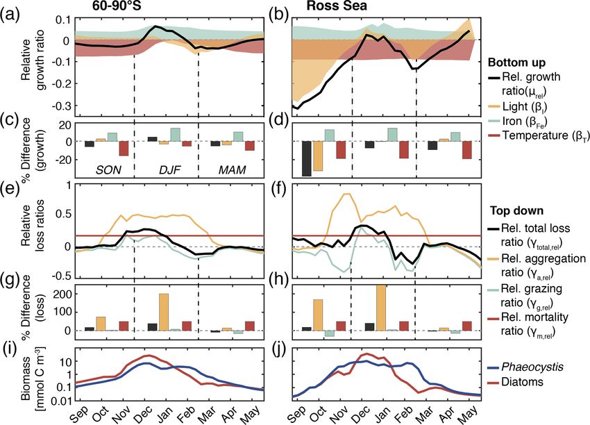
C. Nissen and M. Vogt: Southern Ocean Phaeocystis biogeography                                                                       253

et al., 2011, 2014). Concurrently, while available models         2     Methods
agree with the observations on the general importance of
light and iron levels, differences in the dominant bottom-up      2.1       ROMS-BEC with explicit Phaeocystis colonies
factors controlling the distribution of Phaeocystis at high SO
latitudes across models are possibly a result of differences      We use a quarter-degree SO setup of the Regional Ocean
in how this phytoplankton type is parametrized (Tagliabue         Modeling System (ROMS; latitudinal range from 24–
and Arrigo, 2005; Pasquer et al., 2005; Wang and Moore,           78◦ S, 64 topography-following vertical levels, time step to
2011; Le Quéré et al., 2016; Kaufman et al., 2017; Losa           solve the primitive equations is 1600 s; Shchepetkin and
et al., 2019). In this context, whether the model explicitly      McWilliams, 2005; Haumann, 2016) coupled to the biogeo-
represents both Phaeocystis life stages (Pasquer et al., 2005;    chemical model BEC (Moore et al., 2013), which was re-
Kaufman et al., 2017; Losa et al., 2019) or only the colo-        cently extended to include an explicit representation of coc-
nial stage (Wang and Moore, 2011; Le Quéré et al., 2016)          colithophores and thoroughly validated in the SO setup (Nis-
is key as single cells are known to have lower iron require-      sen et al., 2018). BEC resolves the biogeochemical cycling of
ments than Phaeocystis colonies (Veldhuis et al., 1991). Be-      all macronutrients (C, N, P, Si), as well as the cycling of iron
sides bottom-up factors, some observational studies suggest       (Fe), the major micronutrient in the SO. The model includes
that top-down factors are important in controlling the relative   four PFTs – diatoms, coccolithophores, small phytoplankton
importance of Phaeocystis and diatoms as well. For instance,      (SP), and N2 -fixing diazotrophs – and one zooplankton func-
van Hilst and Smith (2002) suggest grazing by zooplankton         tional type (Moore et al., 2013; Nissen et al., 2018). Here,
to be an important factor explaining the observed distribu-       we extend the version of Nissen et al. (2018) to include an
tions of these two phytoplankton types in the SO, likely re-      explicit parameterization of colonial Phaeocystis antarctica,
sulting from the generally lower grazing pressure on Phaeo-       which is the only bloom-forming species of Phaeocystis oc-
cystis colonies than on diatoms (Granéli et al., 1993; Smith      curring in the SO (Schoemann et al., 2005) and which typ-
et al., 2003). Yet, further evidence suggests a role for other    ically dominates over solitary cells when SO Phaeocystis
biomass loss processes such as aggregation and subsequent         biomass levels are highest (Smith et al., 2003). For the re-
sinking (Asper and Smith, 1999; Ducklow et al., 2015; Asper       mainder of this paper, we will refer to the new PFT as Phaeo-
and Smith, 2019). Altogether, this calls for a comprehensive      cystis. Generally, model parameters for Phaeocystis in the
quantitative analysis of the relative importance of bottom-up     Baseline setup are chosen to represent the colonial form of
and top-down factors in controlling the competition between       Phaeocystis whenever information is available in the litera-
Phaeocystis and diatoms over the course of the SO growing         ture (see, e.g., review by Schoemann et al., 2005), and model
season and its ramifications for carbon transfer to depth.        parameters were tuned to maximize the model–data agree-
   In this study, we investigate the competition between          ment in the spatiotemporal variability of the phytoplankton
Phaeocystis and diatoms and its implications for carbon cy-       community structure between ROMS-BEC and all available
cling using a regional coupled physical–biogeochemical–           observations (see also Sect. 2.3.1). By only simulating the
ecological model configured at eddy-permitting resolution         colonial form of Phaeocystis, we assume enough solitary
for the SO (ROMS-BEC; Nissen et al., 2018). To address            cells of Phaeocystis to be available for colony formation at
the missing link between SO phytoplankton biogeography,           any time as part of the SP PFT. As for the other phytoplank-
ecosystem function, and the global carbon cycle, we have          ton PFTs, growth by Phaeocystis is limited by surrounding
added Phaeocystis colonies as an additional PFT to the            temperature, nutrient, and light conditions as outlined in the
model so that it includes all known biogeochemically rele-        following (see Appendix B for a complete description of the
vant phytoplankton types of the SO (e.g., Buesseler, 1998;        model equations describing phytoplankton growth).
DiTullio et al., 2000). Using available observations, such           As the new PFT in ROMS-BEC represents a single species
as satellite-derived chlorophyll concentrations and carbon        of Phaeocystis, we use an optimum function rather than an
biomass and pigment data, we first validate the simulated         Eppley curve (Eppley, 1972) to describe its temperature-
phytoplankton distributions and community structure across        limited growth rate µPA (T ) (d−1 ; Schoemann et al., 2005):
the SO and then particularly focus on the temporal variabil-                                    T −T
                                                                                                        opt 2

                                                                      PA                   −
ity of diatoms and Phaeocystis in the high-latitude SO. Af-       µ        (T ) = µPA
                                                                                   max · e
                                                                                                   τ
                                                                                                                .                     (1)
ter assessing the relative importance of bottom-up and top-
down factors in controlling the contribution of Phaeocystis       In the above equation, the maximum growth rate (µPA     max ) is
colonies and diatoms to total phytoplankton biomass over a        1.56 d−1 at an optimum temperature (Topt ) of 3.6 ◦ C, and the
complete annual cycle in the high-latitude SO, we show that       temperature interval (τ ) is 17.51 and 1.17 ◦ C at temperatures
the spatially and temporarily varying phytoplankton commu-        below and above 3.6 ◦ C, respectively. With these parameters,
nity composition leaves a distinct, PFT-specific imprint on       the simulated growth rate of Phaeocystis in ROMS-BEC is
upper-ocean carbon cycling and POC export across the SO.          zero at temperatures above ∼ 8 ◦ C (in agreement with lab-
                                                                  oratory experiments with Phaeocystis antarctica; see Buma
                                                                  et al., 1991) and higher than that of diatoms for tempera-

https://doi.org/10.5194/bg-18-251-2021                                                                  Biogeosciences, 18, 251–283, 2021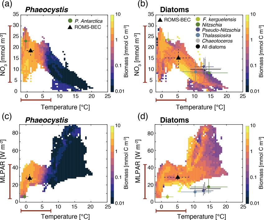
254 C. Nissen and M. Vogt: Southern Ocean Phaeocystis biogeography
Table 1. BEC parameters controlling phytoplankton growth and loss for the five phytoplankton PFTs diatoms (D), Phaeocystis (PA), coccol-
ithophores (C), small phytoplankton (SP), and diazotrophs (DZ). Z is zooplankton, P is phytoplankton, and PI is photosynthesis-irradiance.
If not given in Sect. 2.1, the model equations describing phytoplankton growth and loss rates are given in Nissen et al. (2018).
Parameter Unit Description D PA C SP DZa
µmax d−1 Max. growth rate at 30◦ C 4.6 b 3.8 3.6 0.9
Q10 Temperature sensitivity 1.55 b 1.45 1.5 1.5
kNO3 mmol m−3 Half-saturation constant for NO3 0.5 0.5 0.3 0.1 1.0
kNH4 mmol m−3 Half-saturation constant for NH4 0.05 0.05 0.03 0.01 0.15
kPO4 mmol m−3 Half-saturation constant for PO4 0.05 0.05 0.03 0.01 0.02
kDOP mmol m−3 Half-saturation constant for DOP 0.9 0.9 0.3 0.26 0.09
kFe µmol m−3 Half-saturation constant for Fe 0.15 0.2 0.125 0.1 0.5
kSiO3 mmol m−3 Half-saturation constant for SiO3 1.0 – – – –
αPI mmol C m2 Initial slope of PI-curve 0.44 0.63 0.4 0.44 0.38
mg Chl W s
mg chl
θchl : N, max Max. Chl : N ratio 4.0 2.5 2.5 2.5 2.5
(mmol N)−1
γg,max d−1 Max. growth rate of Z grazing on P 3.8 3.6 4.4 4.4 3.0
zgrz mmol m−3 Half-saturation constant for ingestion 1.0 1.0 1.05 1.05 1.2
γm, 0 d−1 Linear non-grazing mortality 0.12 0.18 0.12 0.12 0.15
γa, 0 m3 Quadratic loss rate in aggregation 0.001 0.005 0.001 0.001 –
mmol C d
rg – Fraction of grazing routed to POC 0.42 0.3 0.2 0.05 0.05
a Compared to Nissen et al. (2018), the k of diazotrophs in ROMS-BEC is higher than for all other PFTs, which is consistent with the literature
Fe
reporting high Fe requirements of Trichodesmium (Berman-Frank et al., 2001). Furthermore, the maximum grazing rate on diazotrophs is lowest
in the model (Capone, 1997). Still, diazotrophs continue to be a minor player in the SO phytoplankton community, contributing < 1 % to
domain-integrated NPP in ROMS-BEC.
b The temperature-limited growth rate of Phaeocystis is calculated based on an optimum function according to Eq. (1) (see also Fig. A1a).
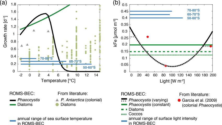
tures between ∼ 0–4 ◦ C (Fig. A1a). We acknowledge that 0.45 µmol m−3 ; see Fig. A1b and Garcia et al., 2009) with the
the range of temperatures for which the growth of Phaeocys- lowest values at optimum light levels of around 80 W m−2 .
tis exceeds that of diatoms is possibly underestimated as the Due to the limited number (three) of reported light levels in
temperature-limited growth rate by diatoms in ROMS-BEC Garcia et al. (2009) and the associated uncertainty when fit-
is overestimated at low temperatures compared to available ting the data, we refrain from using this kFe light dependency
laboratory data (see Fig. A1a and Eq. B5). Yet, we note that in the Baseline simulation but explore the sensitivity of the
temperature-limited growth by diatoms in the model is tuned simulated seasonality of Phaeocystis and diatom biomass to
to fit the data at the global range of temperatures, in particu- a polynomial fit describing the kFe of Phaeocystis as a func-
lar for the competition with coccolithophores at subantarctic tion of the light intensity (see Fig. A1b and Sect. 2.2). As a
latitudes (Nissen et al., 2018). result of the tuning exercise aiming to maximize the fit of all
Half-saturation constants for macronutrient limitation are simulated PFT biomass fields to available observations, the
scarce for P. antarctica (Schoemann et al., 2005), and kFe values of the other PFTs in ROMS-BEC are increased
macronutrient limitation of Phaeocystis is therefore chosen by 25 % in this study as compared to those in Nissen et al.
to be identical to that of diatoms in ROMS-BEC (Table 1). (2018) (see Table 1). For diatoms, this change leads to a bet-
As the availability of the micronutrient Fe generally limits ter agreement of the kFe used in ROMS-BEC with values sug-
phytoplankton growth in the high-latitude SO (Martin et al., gested for large SO diatoms by Timmermans et al. (2004),
1990a, b) and accordingly in ROMS-BEC (Fig. S1), this but we acknowledge that the chosen value here is still at
choice is not expected to significantly impact the simulated the lower end of their suggested range (0.19–1.14 µmol m−3 ).
competition between diatoms and Phaeocystis in this area. In In ROMS-BEC, phytoplankton Fe uptake relative to the up-
contrast, differences in the half-saturation constants with re- take of C varies as a function of seawater Fe levels and de-
spect to dissolved Fe concentrations (kFe ) of Phaeocystis and creases linearly below a critical concentration which is spe-
diatoms critically impact the competitive success of Phaeo- cific to each PFT’s kFe (see Eq. B11). In concert with the
cystis relative to diatoms throughout the year (see, e.g., Sed- seasonal evolution of upper-ocean Fe levels, the Fe : C ratios
wick et al., 2000, 2007). Here, due to their larger size, we of all PFTs are highest in winter and lowest in summer (not
assume a higher kFe for Phaeocystis (0.2 µmol m−3 ) than for shown). As a result of their higher kFe in the model, Phaeo-
diatoms (0.15 µmol m−3 ; Table 1). We note, however, that the cystis generally have lower Fe : C uptake ratios than diatoms.
kFe of Phaeocystis has been reported to vary by over 1 or- We note that we currently do not include any luxury uptake of
der magnitude depending on the ambient light level (0.045– Fe by Phaeocystis into their gelatinous matrix (Schoemann
Biogeosciences, 18, 251–283, 2021 https://doi.org/10.5194/bg-18-251-2021
C. Nissen and M. Vogt: Southern Ocean Phaeocystis biogeography                                                                   255

et al., 2001). Serving as a storage of additional Fe accessi-        by higher trophic levels not explicitly included in ROMS-
ble to the Phaeocystis colony when Fe in the seawater gets           BEC, Phaeocystis in ROMS-BEC experience a higher mor-
low, this luxury uptake is thought to relieve it from Fe lim-        tality rate than diatoms (0.18 and 0.12 d−1 , respectively; see
itation when Fe concentrations become growth limiting (see           γm, 0 in Table 1 and Eq. B16). Thereby, the chosen non-
discussion in Schoemann et al., 2005). We therefore proba-           grazing mortality rate of Phaeocystis assumed in the model
bly overestimate the Fe limitation of Phaeocystis growth in          is still lower than the estimated rate of viral lysis for Phaeo-
ROMS-BEC.                                                            cystis in the North Sea by van Boekel et al. (1992) (0.25 d−1 ),
   P. antarctica blooms are typically found where and when           but we note that data on non-grazing mortality of P. antarc-
waters are turbulent and the mixed layer is deep (in compari-        tica are currently lacking (Schoemann et al., 2005). Further-
son to blooms dominated by diatoms; see, e.g., Arrigo et al.,        more, based on the assumption that for a given biomass con-
1999; Alvain et al., 2008), suggesting that Phaeocystis is bet-      centration, larger cells are more likely than smaller cells to
ter at coping with low light levels than diatoms (e.g., Arrigo       form aggregates and to subsequently stop photosynthesiz-
et al., 1999). In agreement with laboratory experiments (Tang        ing and sink as POC, we use a higher quadratic loss rate for
et al., 2009; Mills et al., 2010; Feng et al., 2010), we there-      Phaeocystis (0.005 d−1 ) than for diatoms (0.001 d−1 ) in the
fore choose a higher αPI , i.e., a higher sensitivity of growth to   model (see γa, 0 in Table 1 and Eq. B18).
increases in photosynthetically active radiation (PAR) at low           In summary, the spatiotemporal variability of the relative
PAR levels, for Phaeocystis than for diatoms in ROMS-BEC             importance of Phaeocystis and diatoms in ROMS-BEC is
(see Table 1). Our value, 0.63 mmol C m2 (mg Chl W s)−1 ,            controlled by the interplay of the environmental conditions
corresponds to the average value compiled from available             and loss processes which differentially impact the growth
laboratory experiments (Schoemann et al., 2005).                     and loss rates of these two PFTs and consequently their com-
   In addition to environmental conditions directly impact-          petitive fitness in the model. In the following, we will de-
ing phytoplankton growth rates, loss processes such as graz-         scribe the model setup and the simulations that were per-
ing, non-grazing mortality, and aggregation impact the sim-          formed to assess the competition between Phaeocystis and
ulated biomass levels at any point and time (Moore et al.,           diatoms throughout the year in the high-latitude SO. The sim-
2002). Grazing on Phaeocystis varies across zooplankton              ulations include a set of sensitivity experiments with the aim
size classes as a consequence of Phaeocystis life forms span-        to assess the impact of choices of single parameters or pa-
ning several orders of magnitude in size (Schoemann et al.,          rameterizations on the simulated Phaeocystis biogeography.
2005). Furthermore, Phaeocystis colonies are surrounded by
a membrane (Hamm et al., 1999), potentially serving as               2.2   Model setup and sensitivity simulations
protection from zooplankton grazing. While small copepods
have been shown to graze less on Phaeocystis once they form          With few exceptions, we use the same ROMS-BEC model
colonies, other larger zooplankton appear to continue grazing        setup as described in detail in Nissen et al. (2018); at the open
on Phaeocystis colonies at unchanged rates (Granéli et al.,          northern boundary, we use monthly climatological fields for
1993; Caron et al., 2000; Schoemann et al., 2005; Nejstgaard         all tracers (Carton and Giese, 2008; Locarnini et al., 2013;
et al., 2007). Based on a size-mismatch assumption of the            Zweng et al., 2013; Garcia et al., 2014b, a; Lauvset et al.,
single grazer in ROMS-BEC and Phaeocystis colonies, we               2016; Yang et al., 2017), and the same data sources are used
assume a lower maximum grazing rate on Phaeocystis than              to initialize the model simulations. At the ocean surface, the
on diatoms (3.6 and 3.8 d−1 , respectively; see γg,max in Ta-        model is forced with a 2003 normal year forcing for momen-
ble 1). Upon grazing, we assume the fraction of the grazed           tum, heat, and freshwater fluxes (Dee et al., 2011). Satellite-
phytoplankton biomass that is transformed to sinking POC             derived climatological total chlorophyll concentrations are
via zooplankton fecal pellet production to be higher for larger      used to initialize phytoplankton biomass and to constrain it
and ballasted cells than for small, unballasted cells. Conse-        at the open northern boundary in the model (NASA-OBPG,
quently, the fraction of grazing routed to POC increases from        2014b), and the fields are extrapolated to depth following
grazing on SP or diazotrophs to coccolithophores, Phaeocys-          Morel and Berthon (1989). Due to the addition of Phaeo-
tis, and diatoms (rg in Table 1). Consistent with Nissen et al.      cystis, the partitioning of total chlorophyll onto the different
(2018), we keep a Holling type II ingestion functional re-           phytoplankton PFTs is adjusted compared to Nissen et al.
sponse here (Holling, 1959) and compute grazing on each              (2018): 90 % is attributed to small phytoplankton, 4 % to both
prey separately (Eq. B14). We refer to Nissen et al. (2018)          diatoms and coccolithophores, and 1 % to both diazotrophs
for a discussion of the relative merits and pitfalls for using       and Phaeocystis. This partitioning is motivated by the phy-
Holling type II vs. III.                                             toplankton community structure at the open northern bound-
   Non-grazing mortality (such as viral lysis) has been              ary at 24◦ S, where small phytoplankton typically dominate
shown to increase under environmental stress for Phaeocystis         and P. antarctica are only a minor contributor to phytoplank-
colonies, causing colony disruption and ultimately cell death        ton biomass (see, e.g., Schoemann et al., 2005; Swan et al.,
(van Boekel et al., 1992; Schoemann et al., 2005). To account        2016). Phaeocystis is initialized with a carbon-to-chlorophyll
for processes causing colony disintegration and for grazing          ratio of 60 mg C (mg chl)−1 (same as small phytoplankton

https://doi.org/10.5194/bg-18-251-2021                                                         Biogeosciences, 18, 251–283, 2021
256                                                            C. Nissen and M. Vogt: Southern Ocean Phaeocystis biogeography

Table 2. Overview of sensitivity experiments aiming to (1) assess the sensitivity of the simulated Phaeocystis–diatom competition to chosen
parameter values and parameterizations of Phaeocystis (competition experiments, runs 1–8) and (2) assess the sensitivity of the simulated
biomass distributions to chosen Phaeocystis parameter values (parameter sensitivity experiments, runs 9–22). The results of the parameter
sensitivity experiments are discussed in the Supplement. See Table 1 and Sect. 2.1 for parameter values and parameterizations of Phaeocystis
in the reference simulation. PA is Phaeocystis, and D is diatoms.

           Competition        Run name           Description
                                                                                            T −Tref
           1                  TEMPERATURE Use µD        D         PA     D         D 10 ◦ C to compute the temperature-
                                                 max , Q10 , and µT = µmax × Q10
                                          limited growth rate of Phaeocystis instead of Eq. (1)

           2                  ALPHAPI                 PA to α D
                                                 Set αPI     PI

           3                  IRON                    PA to k D
                                                 Set kFe     Fe

           4                  GRAZING                 PA
                                                 Set γg,max     D
                                                            to γmax

           5                  AGGREGATION Set γa,PA0 to γa,D0

           6                  MORTALITY               PA to γ D
                                                 Set γm, 0   m, 0

           7                                   PA
                              THETA_N_MAX Set θchl              D
                                                   : N, max to θchl : N, max

           8                  VARYING_kFE              PA (I ) = 2.776 × 10⁻⁵ × (I + 20)2 − 0.00683 × (I + 20) + 0.46 (with the
                                                 Use kFe
                                                                                                PA
                                                 irradiance I in W m−2 ) instead of a constant kFe
           Parameter          Run name           Description
           sensitivity
           9                  Topt150                      PA by 50 %
                                                 Increase Topt

           10                 Topt50                      PA by 50 %
                                                 DecreaseTopt

           11                 kFe150                       PA by 50 %
                                                 Increase kFe

           12                 kFe50                        PA by 50 %
                                                 Decrease kFe

           13                 alphaPI150                   PA by 50 %
                                                 Increase αPI

           14                 alphaPI50                    PA by 50 %
                                                 Decrease αPI

           15                 mortality150                 PA by 50 %
                                                 Increase γm, 0

           16                 mortality50                  PA by 50 %
                                                 Decrease γm, 0

           17                 aggregation150     Increase γa,PA0 by 50 %

           18                 aggregation50      Decrease γa,PA0 by 50 %

           19                 grazing150                   PA
                                                 Increase γg,max by 50 %

           20                 grazing50                    PA
                                                 Decrease γg,max by 50 %

           21                 thetaNmax150                 PA
                                                 Increase θchl : N, max by 50 %

           22                 thetaNmax50                  PA
                                                 Decrease θchl : N, max by 50 %

Biogeosciences, 18, 251–283, 2021                                                             https://doi.org/10.5194/bg-18-251-2021
C. Nissen and M. Vogt: Southern Ocean Phaeocystis biogeography                                                                   257

and coccolithophores), whereas diatoms are initialized with          2.3     Data and diagnostics used in the model assessment
a ratio of 36 mg C (mg chl)−1 (Sathyendranath et al., 2009).
   We first run a 30-year-long physics-only spin-up, followed        2.3.1    Evaluating the simulated phytoplankton
by a 10-year-long spin-up in the coupled ROMS-BEC setup.                      community structure
Our Baseline simulation for this study is then run for an ad-
ditional 10 years, of which we analyze a daily climatology           We compare the simulated spatiotemporal variability in phy-
over the last five full seasonal cycles, i.e., from 1 July of year   toplankton biomass and community structure to available ob-
5 until 30 June of year 10. Apart from having added Phaeo-           servations of phytoplankton carbon biomass concentrations
cystis and adjustments to the parameters of the other PFTs as        from the MAREDAT initiative (O’Brien et al., 2013; Leblanc
described in Sect. 2.1, the setup of the Baseline simulation         et al., 2012; Vogt et al., 2012), satellite-derived total chloro-
in this study is thereby identical to the Baseline simulation        phyll concentrations (Fanton d’Andon et al., 2009; Mari-
in Nissen et al. (2018). We will evaluate the model’s perfor-        torena et al., 2010), DMS measurements (Curran and Jones,
mance with respect to the simulated phytoplankton biogeog-           2000; Lana et al., 2011), the ecological niches suggested for
raphy in Sect. 3.1 and in the Supplement.                            SO phytoplankton taxa (Brun et al., 2015), and the CHEM-
   Furthermore, we perform two sets of sensitivity experi-           TAX climatology based on high-performance liquid chro-
ments (22 simulations in total) in order to (1) assess the sen-      matography (HPLC) pigment data (Swan et al., 2016). The
sitivity of the simulated Phaeocystis biogeography and the           latter provides seasonal estimates of the mixed-layer average
competition of Phaeocystis and diatoms to chosen param-              community composition, which we compare to the season-
eters and parameterizations (competition experiments, runs           ally and top 50 m averaged model output of each phytoplank-
1–8 in Table 2) and (2) systematically assess the sensitiv-          ton’s contribution to total chlorophyll biomass. The CHEM-
ity of the simulated biomass distributions to chosen Phaeo-          TAX analysis splits the phytoplankton community into di-
cystis parameter values (parameter experiments, runs 9–22).          atoms, nitrogen fixers (such as Trichodesmium), picophyto-
For the former set, we set the parameters and parameteriza-          plankton (such as Synechococcus and Prochlorococcus), di-
tions of Phaeocystis to those used for diatoms in ROMS-BEC           noflagellates, cryptophytes, chlorophytes (all three combined
(runs 1–8 in Table 2). Generally, the differences in parame-         into the single group “Others” here), and haptophytes (such
ters between Phaeocystis and diatoms affect either the sim-          as coccolithophores and Phaeocystis). As noted in Swan
ulated biomass accumulation rates (runs TEMPERATURE,                 et al. (2016), the differentiation between coccolithophores
ALPHAPI , IRON, and THETA_N_MAX) or loss rates (runs                 and Phaeocystis in the CHEMTAX analysis is difficult and
GRAZING, AGGREGATION, and MORTALITY). By suc-                        prone to error. Possibly, this is due to the large variability
cessively eradicating the differences between Phaeocystis            in pigment composition of Phaeocystis in response to vary-
and diatoms, these simulations allow us to directly quantify         ing environmental conditions, especially regarding light and
the impact of parameter differences on the simulated relative        iron levels (Smith et al., 2010; Wright et al., 2010). Coc-
importance of Phaeocystis for total phytoplankton biomass.           colithophores have been reported to only grow very slowly
To assess the impact of iron–light interactions on the com-          at low temperatures (below ∼ 8 ◦ C; Buitenhuis et al., 2008),
petitive success of Phaeocystis at high SO latitudes, we ul-         and in the SO, their abundance at the high latitudes south of
timately run a simulation in which the half-saturation con-          the polar front is very low (Balch et al., 2016). Therefore,
stant of iron (kFe ) of Phaeocystis is a function of the light       whenever the climatological temperature in the World Ocean
intensity following a polynomial fit of available laboratory         Atlas 2013 (Locarnini et al., 2013) is below 2 ◦ C at the time
data (VARYING_kFE; Fig. A1b; Garcia et al., 2009). For the           and location of the respective HPLC observation, we reas-
second set of experiments, we systematically vary Phaeocys-          sign data points identified as “Hapto-6” (hence, e.g., Emilia-
tis growth and loss parameters by ±50 %, and the results of          nia huxleyi) in the CHEMTAX analysis to “Hapto-8” (hence,
these experiments are discussed in detail in section S2 of the       e.g., Phaeocystis antarctica). Throughout the paper, this new
Supplement. All sensitivity experiments use the same physi-          category (“Hapto-8 reassigned”) is indicated separately in
cal and biogeochemical spin-up as the Baseline simulation            the respective figures and leads to a better correspondence
and start from the end of year 10 of the coupled ROMS-               between the functional types included in the CHEMTAX-
BEC spin-up. Each simulation is then run for an additional           based climatology by Swan et al. (2016) and the PFTs in
10 years, of which the average over the last five full seasonal      ROMS-BEC.
cycles is analyzed in this study.                                       To assess the controlling factors of the simulated PFT dis-
                                                                     tributions in our model, we analyze the simulated summer
                                                                     (December–March; DJFM) top 50 m average biomass dis-
                                                                     tribution of the different model PFTs south of 40◦ S in en-
                                                                     vironmental niche space. To that aim, we bin the simulated
                                                                     carbon biomass concentrations of Phaeocystis, diatoms, and
                                                                     coccolithophores in ROMS-BEC as a function of the temper-
                                                                     ature (◦ C), nitrate concentration (mmol m−3 ), iron concentra-

https://doi.org/10.5194/bg-18-251-2021                                                         Biogeosciences, 18, 251–283, 2021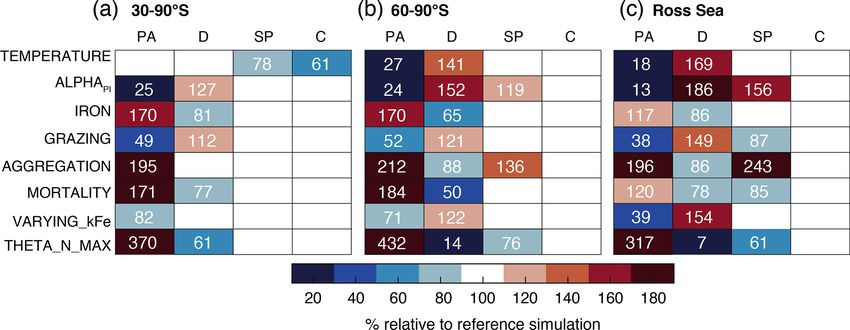
258                                                         C. Nissen and M. Vogt: Southern Ocean Phaeocystis biogeography

tion (µmol m−3 ), and mixed-layer photosynthetically active          grazing mortality γmi , and aggregation γai ; see Appendix B
radiation (MLPAR; W m−2 ). Subsequently, we compare the              for a full description of the model equations). Here, in order
simulated ecological niche to that observed for abundant SO          to disentangle the factors controlling the relative importance
species of each model PFT (such as Phaeocystis antarctica,           of Phaeocystis and diatoms for total phytoplankton biomass
Fragilariopsis kerguelensis, Thalassiosira sp., or Emiliania         throughout the year, we use the metrics first introduced by
huxleyi; see Brun et al., 2015). In Sect. 3.3 of this paper, only    Hashioka et al. (2013) and then applied to assess the competi-
the results for Phaeocystis and diatoms will be shown, the           tion of diatoms and coccolithophores in ROMS-BEC in Nis-
corresponding figures for coccolithophores can be found in           sen et al. (2018). Same as in Nissen et al. (2018), the relative
                                                                                      ij
the Supplement (Figs. S2 and S3). While this analysis in-            growth ratio µrel of phytoplankton i and j (e.g., diatoms and
forms on possible links between the competitive fitness of a         Phaeocystis) is defined as the ratios of their specific growth
PFT and the environmental conditions it lives in, the assess-        rates (µi , d−1 ), which in turn depends on environmental de-
ment is limited to a qualitative intercomparison due to diffi-       pendencies regarding the temperature T , nutrients N, and ir-
culties in comparing a model PFT to individual phytoplank-           radiance I , as follows:
ton species, a sampling bias towards the summer months and                      µD
the low latitudes, and the neglect of loss processes such as         µDPA
                                                                      rel = log
                                                                               µPA
zooplankton grazing to explain biomass distributions. As a
consequence, the ecological niche analysis does not allow for              f (T ) · µD
                                                                            D
                                                                                     max       g D (N )        hD (I )
                                                                     = log               + log           + log          .            (2)
the assessment of any temporal variability in PFT biomass                      µPA             g PA (N )       hPA (I )
concentrations.                                                        |      {z T     } | {z } | {z }
                                                                                  βT                   βN ∼βFe        βI
    In order to assess the simulated seasonality and the sea-
sonal succession of Phaeocystis and diatoms, we identify the         In the above equation, the specific growth rate µi of each
bloom peak as the day of peak chlorophyll concentrations             phytoplankton i is calculated as a multiplicative function of
throughout the year. Besides the timing of the bloom peak,           a temperature-limited growth rate (f D (T ) · µD   max for diatoms
phytoplankton phenology is typically characterized by met-           and µPAT  for  Phaeocystis;  see Eqs.   B5 and   1), a nutrient lim-
rics such as the day of bloom initiation or the day of bloom         itation term (g i (N ), limitation of each nutrient is calculated
end (see, e.g., Soppa et al., 2016). In this regard, the timing      using a Michaelis–Menten function, and the most-limiting
of the bloom start is known to be sensitive to the chosen iden-      one is then used here; see Eq. B8), and a light limitation
tification methodology (Thomalla et al., 2015). At high lati-        term (hi (I ); see Eq. B9 and Geider et al., 1998). Further, βT ,
tudes, the identification of the bloom start based on remotely       βN , and βI describe the logarithmic ratio of the limitation by
sensed chlorophyll concentrations is additionally impaired           temperature, nutrients, and light of growth by diatoms and
by the large amount of missing data in all seasons (even in          Phaeocystis. Thereby, these terms denote the log-normalized
the summer months, a large part of the SO is sampled by the          contribution of each environmental factor to the simulated
satellite for less than 5 of the 21 available years; see Fig. S4),   relative growth ratio. At high latitudes south of 60◦ S, the
complicating any comparison of the high-latitude satellite-          ratio of the nutrient limitation of growth βN corresponds to
derived bloom start with output from models such as ROMS-            that of the iron limitation βFe in our model (Fig. S1). Con-
BEC. To minimize the uncertainty due to the low data cover-          sequently, environmental conditions regarding temperature,
age in the region of interest for this study and as the seasonal     iron, and light decide whether the relative growth ratio is pos-
succession of Phaeocystis and diatoms in the high-latitude           itive or negative at a given location and point in time, i.e.,
SO is mostly inferred from the timing of observed maximum            which of the two phytoplankton types has a higher specific
abundances in the literature (e.g., Peloquin and Smith, 2007;        growth rate and hence a competitive advantage over the other
Smith et al., 2011), we focus our discussion of the simulated        regarding growth.
                                                                                                                  ij
bloom phenology on the timing of the bloom peak (Hash-                  Similarly, the relative grazing ratio γg,rel of phytoplankton
ioka et al., 2013). To evaluate the model’s performance, we          i and j (e.g., diatoms and Phaeocystis) is defined as the ratio
compare the timing of the total chlorophyll bloom peak in            of their specific grazing rates (γgi , d−1 ), as follows:
the Baseline simulation of ROMS-BEC to the bloom tim-                                 γgPA
ing derived from climatological daily chlorophyll data from           DPA             P PA
Globcolor (climatology from 1998–2018 based on the daily             γg,rel   = log          .                                       (3)
                                                                                      γgD
25 km chlorophyll product; see Fanton d’Andon et al., 2009;                           PD
Maritorena et al., 2010).                                            In ROMS-BEC, grazing on each phytoplankton i is calcu-
                                                                     lated using a Holling type II ingestion function (Nissen et al.,
2.3.2   Phytoplankton competition and succession                     2018). As described in Sect. 2.1, Phaeocystis and diatoms
                                                                     in ROMS-BEC do not only differ in parameters describing
In ROMS-BEC, phytoplankton biomass P i (mmol C m−3 ,                 the zooplankton grazing pressure they experience but in pa-
i ∈ {PA, D, C, SP, N}) is determined by the balance between          rameters describing their non-grazing mortality and aggrega-
growth (µi ) and loss terms (grazing by zooplankton γgi , non-       tion losses as well. Therefore, in accordance with the relative

Biogeosciences, 18, 251–283, 2021                                                                https://doi.org/10.5194/bg-18-251-2021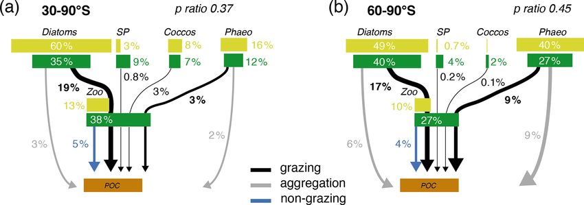
C. Nissen and M. Vogt: Southern Ocean Phaeocystis biogeography                                                                    259

grazing ratio defined above, we define the relative mortal-           the model overestimates annual mean satellite-derived sur-
            ij                                            ij
ity ratio (γm,rel ) and the relative aggregation ratio (γa,rel ) of   face chlorophyll biomass estimates by 18 % (40.8 Gg chl
phytoplankton i and j (e.g., diatoms and Phaeocystis) as the          in ROMS-BEC between 30–90◦ S compared to 34.5 Gg chl
ratio of their specific non-grazing mortality rates (γmi , d−1 )      in the MODIS Aqua chlorophyll product; Table 3; NASA-
and aggregation rates (γai , d−1 ), respectively, as follows:         OBPG, 2014a; Johnson et al., 2013) and satellite-derived
                                                                      NPP by 38 %–42 % (17.2 compared to 12.1–12.5 Pg C yr−1 ;
                 γmPA                                                 Table 3; Behrenfeld and Falkowski, 1997; O’Malley, 2016;
 DPA             P PA
γm,rel   = log          ,                                      (4)    Buitenhuis et al., 2013). This bias is largest south of 60◦ S
                 γmD
                 PD                                                   where NPP and surface chlorophyll are overestimated by a
                 γaPA                                                 factor of 1.8–4.4 and 1.8, respectively (Table 3), and the
 DPA             P PA                                                 bias is likely due to a combination of underestimated high-
γa,rel = log            .                                      (5)
                 γaD                                                  latitude chlorophyll concentrations in satellite-derived prod-
                 PD
                                                                      ucts (Johnson et al., 2013) and the missing complexity in
                                            ij
Since the total specific loss rate (γtotal , d−1 ) of phytoplankton   the zooplankton compartment in ROMS-BEC as biases in
i is the addition of its specific grazing and non-grazing mor-        the simulated physical fields (temperature, light) have been
tality and aggregation loss rates, the relative total loss ratio      shown to only explain a minor fraction of the simulated high-
  ij
γtotal,rel of phytoplankton i and j (e.g., diatoms and Phaeo-         latitude biomass overestimation (Nissen et al., 2018).
cystis) is defined as                                                    The simulated carbon biomass distributions of colonial
                                                                      Phaeocystis, diatoms, coccolithophores, and SP are distinct
                   γgPA   γmPA   γaPA                                 in the model (Fig. 1c–f, showing top 50 m averages). The
  DPA              P PA + P PA + P PA                                 simulated summer Phaeocystis biomass is highest south of
γtotal,rel = log                        .                      (6)
                    γgD   γmD    γaD                                  50◦ S with the highest concentrations of 10 mmol C m−3 at
                    PD
                        + PD + PD
                                                                      ∼ 74◦ S. In the model, average Phaeocystis biomass concen-
     DPA                                                              trations quickly decline to levels < 0.1 mmol C m−3 north of
If γtotal,rel is positive, the specific total loss rate of Phaeo-
                                                                      50◦ S (Fig. 1c), a direct result of the restriction of Phaeocys-
cystis is larger than that of diatoms (and accordingly for the
                                                                      tis growth to temperatures  20 mmol C m−3 ) south
Phaeocystis. While the maximum grazing rate on Phaeocys-
                                                                      of ∼ 75◦ S and concentrations < 5 mmol C m−3 north of ∼
tis is lower than that of diatoms, their non-grazing mortality
                                                                      65◦ S (Figs. 1c and S5a and b). As a response to the addition
and aggregation losses are higher (see Sect. 2.1 and Table 1).
                                                                      of Phaeocystis to ROMS-BEC, the simulated high-latitude
Ultimately, at any given location and point in time, the in-
                                                                      diatom biomass concentrations decrease compared to the 4-
teraction between the phytoplankton biomass concentrations
                                                                      PFT setup of the model (Nissen et al., 2018). In the 5-PFT
(impacting the respective loss rates) and environmental con-
                                                                      setup, the model simulates the highest diatom biomass south
ditions (impacting the respective growth rate) will determine
                                                                      of 60◦ S with maximum concentrations of ∼ 7 mmol C m−3
the relative contribution of each phytoplankton type i to to-
                                                                      at 72◦ S (top 50 m mean; ∼ 17 mmol C m−3 in 4-PFT setup)
tal phytoplankton biomass. Here, we use these metrics to as-
                                                                      and rapidly declining concentrations north of 60◦ S (Fig. 1d).
sess the controls on the simulated seasonal evolution of the
                                                                      Nevertheless, the simulated summer diatom biomass lev-
relative importance of Phaeocystis and diatoms in the high-
                                                                      els are still overestimated compared to carbon biomass es-
latitude SO.
                                                                      timates (Fig. S5c; Leblanc et al., 2012) and satellite-derived
                                                                      diatom chlorophyll estimates (Soppa et al., 2014) (compari-
3     Results                                                         son not shown). In contrast to both Phaeocystis and diatoms,
                                                                      the simulated biomass levels of coccolithophores are highest
3.1      Phytoplankton biogeography and community                     in the subantarctic (highest concentrations of 3 mmol C m−3
         composition in the SO                                        on the Patagonian Shelf; Figs. 1e and S3d). Overall, their
                                                                      simulated SO biogeography agrees well with the position
In the 5-PFT Baseline simulation of ROMS-BEC, total sum-              of the Great Calcite Belt (Balch et al., 2011, 2016) and re-
mer chlorophyll is highest close to the Antarctic continent           mains largely unchanged compared to the 4-PFT setup (Nis-
(> 10 mg chl m−3 ) and decreases northwards to values <               sen et al., 2018).
1 mg chl m−3 close to the open northern boundary (Fig. 1a).              Taken together, the model simulates a phytoplankton com-
While this south–north gradient is in broad agreement with            munity with substantial contributions of coccolithophores
remotely sensed chlorophyll concentrations (Fig. 1b), our             and Phaeocystis in the subantarctic and high-latitude SO,
model generally overestimates high-latitude chlorophyll lev-          respectively (Fig. 2a). CHEMTAX data generally support
els, which has already been noted for the 4-PFT setup of              this latitudinal trend (see Fig. 2b–d and Sect. 2.3.1; Swan
ROMS-BEC (Nissen et al., 2018). With Phaeocystis added,               et al., 2016). Averaged over 30–90◦ S (60–90◦ S), the simu-

https://doi.org/10.5194/bg-18-251-2021                                                          Biogeosciences, 18, 251–283, 2021
260 C. Nissen and M. Vogt: Southern Ocean Phaeocystis biogeography Figure 1. Biomass distributions for December–March (DJFM). Total surface chlorophyll (mg chl m−3 ) in (a) ROMS-BEC and (b) MODIS- Aqua climatology (NASA-OBPG, 2014a) using the chlorophyll algorithm by Johnson et al. (2013). (c, f) Mean top 50 m (c) Phaeocystis, (d) diatom, (e) coccolithophore, and (f) small phytoplankton carbon biomass concentrations (mmol C m−3 ) in ROMS-BEC. Phaeocystis, diatom, and coccolithophore biomass observations from the top 50 m are indicated by colored dots in (c), (d), and (e), respectively (Balch et al., 2016; Saavedra-Pellitero et al., 2014; O’Brien et al., 2013; Vogt et al., 2012; Leblanc et al., 2012; Tyrrell and Charalampopoulou, 2009; Gravalosa et al., 2008; Cubillos et al., 2007). For more details on the biomass evaluation, see Nissen et al. (2018). lated relative contributions of Phaeocystis, diatoms, and coc- CHEMTAX to the Phaeocystis PFT in ROMS-BEC have to colithophores to total chlorophyll in summer are 20 ± 28 % be noted (see Sect. 2.3.1). (33 ± 34 %; subarea mean as shown in Fig. 2b and c ±1σ in In the 4-PFT setup of ROMS-BEC, the simulated sum- space), 68 ± 33 % (64 ± 33 %), and 5 ± 17 % (< 1 ± 2 %), re- mer phytoplankton community south of 60◦ S was often al- spectively, which is in good agreement with the CHEMTAX most solely composed of diatoms (Fig. S6 and Nissen et al., climatology: 28 % (27 %), 46 % (48 %), and 3 % (1 %), re- 2018), suggesting that the implementation of Phaeocystis led spectively. Acknowledging the uncertainty in the attribution to a substantial improvement in the representation of the ob- of the group “Others” in the CHEMTAX data to a model PFT served high-latitude community structure (Fig. 2). Concur- (Others includes dinoflagellates, cryptophytes, and chloro- rently, as the distribution of silicic acid and nitrate is directly phytes here; see Sect. 2.3.1), the model also captures the impacted by the relative importance of silicifying and non- seasonal evolution of the relative importance of Phaeocys- silicifying phytoplankton, such as Phaeocystis, in the com- tis and diatoms reasonably well, both averaged over 30– munity, the addition of Phaeocystis to the model led to an 90◦ S (Fig. 2b) and at high SO latitudes (Fig. 2c–d). The improvement in the simulated high-latitude nutrient distribu- model overestimates the contribution of Phaeocystis in fall tions compared to climatological data from the World Ocean (39 ± 14 % as compared to 24 % in CHEMTAX) and spring Atlas (WOA; Fig. S7d–f and Garcia et al., 2014b). Upon (51 ± 22 % as compared to 28 %) between 60–90◦ S and in the addition of Phaeocystis, the zonal average location of the Ross Sea, respectively (Fig. 2c–d), but the limited num- the silicate front, i.e., the latitude at which nitrate and sili- ber of data points available in the CHEMTAX climatology in cic acid concentrations are equal (Freeman et al., 2018), is this area and the uncertainty in the attribution of pigments in shifted northward by ∼ 7 ◦ in ROMS-BEC (from 57.1◦ S in Biogeosciences, 18, 251–283, 2021 https://doi.org/10.5194/bg-18-251-2021
C. Nissen and M. Vogt: Southern Ocean Phaeocystis biogeography                                                                                               261

Table 3. Comparison of ROMS-BEC-based phytoplankton biomass, production, and export estimates with available observations (given in
parentheses). Data sources are given below the table. The reported uncertainty of the contribution of the PFTs to the simulated integrated
NPP corresponds to the area-weighted spatial variability of each PFT’s contribution to annual NPP (1σ in space).

                                                                                                                  ROMS-BEC (data)
                                                                                                                    30–90◦ S                   60–90◦ S
           Surface chlorophyll biomass                 Total, annual mean (Gg chl)                                 40.8 (34.5a )              17.1 (9.5a )
           Diatom carbon biomass                       0–200 m, annual mean (Pg C)               0.059 (globalb : 0.10–0.94)                       0.015
           Phaeocystis carbon biomass                  0–200 m, annual mean (Pg C)              0.019 (globalb : 0.11–0.71)                        0.010
           Coccolithophore carbon biomass              0–200 m, annual mean (Pg C)             0.012 (globalb : 0.001–0.03)                        0.001
           NPP                                         Pg C yr−1                                         17.2 (12.1–12.5c )              3.0 (0.68–1.7c )
                                                       Diatoms (%)                                             52.0 (±26.2)                49.1 (±19.9)
                                                       Phaeocystis (%)                                         15.3 (±24.5)                45.8 (±20.7)
                                                       Coccolithophores (%)                                    14.6 (±15.3)                   0.7 (±1.0)
                                                       SP (%)                                                  17.2 (±16.1)                   4.5 (±1.9)
           POC export at 100 m                         Pg C yr−1                                           3.1 (2.3–2.96d )           0.62 (0.21–0.24d )
         a Monthly climatology from MODIS Aqua (2002–2016; NASA-OBPG, 2014a) SO algorithm (Johnson et al., 2013).
         b The reported estimates from the MAREDAT database in Buitenhuis et al. (2013) are global estimates of phytoplankton biomass.
         c Monthly climatology from MODIS Aqua vertically generalized production model (VGPM; 2002–2016; Behrenfeld and Falkowski, 1997; O’Malley,
         2016). NPP climatology from Buitenhuis et al. (2013) (2002–2016).
         d Monthly output from a biogeochemical inverse model (Schlitzer, 2004) and a data-assimilated model (DeVries and Weber, 2017).

4-PFT setup to 50◦ S in 5-PFT setup; see Fig. S8). While                               phyll levels (see dashed red and green lines in Fig. S9a),
this is further north than suggested by WOA data (56.5◦ S;                             suggesting that biological factors must explain the difference
Fig. S8b and Garcia et al., 2014b), this can certainly be ex-                          between ROMS-BEC and the satellite product. As diatoms
pected to affect the competitive fitness of individual phyto-                          dominate the phytoplankton community at peak total chloro-
plankton types in the subantarctic and possibly at lower lati-                         phyll concentrations for all latitudinal averages in the model
tudes, which we did not assess further in this study. Overall,                         domain (compare their bloom timing in Fig. 3a–c with the
our model agrees with observational data that Phaeocystis                              simulated community composition in Fig. 2b–d, but note that
is an important member of the high-latitude phytoplankton                              Phaeocystis often dominate in coastal areas; not shown), the
community. In the remainder of the paper, we will therefore                            mismatch in timing is likely related to the representation of
explore the temporal variability in the relative importance of                         this PFT in the model and is possibly at least partly caused
diatoms and Phaeocystis and its implications for SO carbon                             by their comparatively high growth rates at low temperatures
cycling in more detail.                                                                (see Fig. A1a).
                                                                                          In contrast to diatoms, maximum zonally averaged chloro-
3.2   Phytoplankton phenology and the seasonal                                         phyll concentrations of Phaeocystis are simulated for late
      succession of Phaeocystis and diatoms                                            November or early December across most latitudes in the
                                                                                       model (only at around 70◦ S is a peak in late January sim-
Maximum total chlorophyll concentrations are simulated for                             ulated; Fig. 3b; note that locally, maximum Phaeocystis
the first half of December across latitudes in ROMS-BEC                                chlorophyll concentrations exceed 10 mg chl m−3 ; not shown
(solid blue line in Fig. 3a) and at high SO latitudes south of                         here). Overall, the timing of simulated peak Phaeocystis
60◦ S, total chlorophyll blooms start already in late Septem-                          chlorophyll levels corresponds well with the suggested tim-
ber in the model (not shown). Thereby, the model-derived                               ing of observed maximum seawater dimethylsulfoniopropi-
timing of total chlorophyll bloom start and peak is 2–3 and                            onate (DMSP) concentrations (peak in November/December
1–2 months earlier, respectively, than satellite-derived esti-                         in Curran et al., 1998; Curran and Jones, 2000) and the
mates (for bloom peak, see black line in Fig. 3a; for bloom                            delayed maximum atmospheric DMS concentrations (Jan-
start, see, e.g., Thomalla et al., 2011). Yet, compared to the 4-                      uary/February; e.g., Nguyen et al., 1990; Ayers et al., 1991).
PFT setup (dashed blue line in Fig. 3a), the simulated timing                          This further corroborates the hypothesis that the bias in the
of peak chlorophyll levels improved in this study, with peak                           timing of maximum total chlorophyll levels in ROMS-BEC
chlorophyll delayed by on average 1 week in the model upon                             is likely caused by how diatoms are parameterized in the
the implementation of Phaeocystis. The simulated physical                              model (see, e.g., the rather high temperature-limited growth
biases (i.e., generally temperatures too high and mixed-layer                          rate of diatoms at low temperatures compared to available
depths too shallow, both favoring an earlier onset of the phy-                         laboratory data; see Fig. A1). Taken together, the model sim-
toplankton bloom; see Nissen et al., 2018) only partially ex-                          ulates a succession from Phaeocystis to diatoms close to the
plain the bias in the simulated timing of maximum chloro-                              Antarctic continent (south of 72◦ S; see also Fig. S9b) and

https://doi.org/10.5194/bg-18-251-2021                                                                                  Biogeosciences, 18, 251–283, 2021
You can also read