An improved global remote-sensing-based surface soil moisture (RSSSM) dataset covering 2003-2018 - ESSD
←
→
Page content transcription
If your browser does not render page correctly, please read the page content below
Earth Syst. Sci. Data, 13, 1–31, 2021
https://doi.org/10.5194/essd-13-1-2021
© Author(s) 2021. This work is distributed under
the Creative Commons Attribution 4.0 License.
An improved global remote-sensing-based surface soil
moisture (RSSSM) dataset covering 2003–2018
Yongzhe Chen1,2 , Xiaoming Feng1 , and Bojie Fu1,2
1 StateKey Laboratory of Urban and Regional Ecology, Research Center for Eco-Environmental Sciences,
Chinese Academy of Sciences, Beijing 100085, China
2 College of Resources and Environment, University of Chinese Academy of Sciences, Beijing 100049, China
Correspondence: Xiaoming Feng (fengxm@rcees.ac.cn)
Received: 9 March 2020 – Discussion started: 8 May 2020
Revised: 13 November 2020 – Accepted: 18 November 2020 – Published: 5 January 2021
Abstract. Soil moisture is an important variable linking the atmosphere and terrestrial ecosystems. However,
long-term satellite monitoring of surface soil moisture at the global scale needs improvement. In this study, we
conducted data calibration and data fusion of 11 well-acknowledged microwave remote-sensing soil moisture
products since 2003 through a neural network approach, with Soil Moisture Active Passive (SMAP) soil moisture
data applied as the primary training target. The training efficiency was high (R 2 = 0.95) due to the selection of
nine quality impact factors of microwave soil moisture products and the complicated organizational structure of
multiple neural networks (five rounds of iterative simulations, eight substeps, 67 independent neural networks,
and more than 1 million localized subnetworks). Then, we developed the global remote-sensing-based surface
soil moisture dataset (RSSSM) covering 2003–2018 at 0.1◦ resolution. The temporal resolution is approximately
10 d, meaning that three data records are obtained within a month, for days 1–10, 11–20, and from the 21st to
the last day of that month. RSSSM is proven comparable to the in situ surface soil moisture measurements of
the International Soil Moisture Network sites (overall R 2 and RMSE values of 0.42 and 0.087 m3 m−3 ), while
the overall R 2 and RMSE values for the existing popular similar products are usually within the ranges of 0.31–
0.41 and 0.095–0.142 m3 m−3 ), respectively. RSSSM generally presents advantages over other products in arid
and relatively cold areas, which is probably because of the difficulty in simulating the impacts of thawing and
transient precipitation on soil moisture, and during the growing seasons. Moreover, the persistent high quality
during 2003–2018 as well as the complete spatial coverage ensure the applicability of RSSSM to studies on
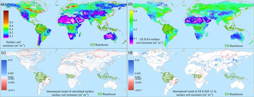
both the spatial and temporal patterns (e.g. long-term trend). RSSSM data suggest an increase in the global mean
surface soil moisture. Moreover, without considering the deserts and rainforests, the surface soil moisture loss on
consecutive rainless days is highest in summer over the low latitudes (30◦ S–30◦ N) but mostly in winter over the
mid-latitudes (30–60◦ N, 30–60◦ S). Notably, the error propagation is well controlled with the extension of the
simulation period to the past, indicating that the data fusion algorithm proposed here will be more meaningful
in the future when more advanced microwave sensors become operational. RSSSM data can be accessed at
https://doi.org/10.1594/PANGAEA.912597 (Chen, 2020).
Published by Copernicus Publications.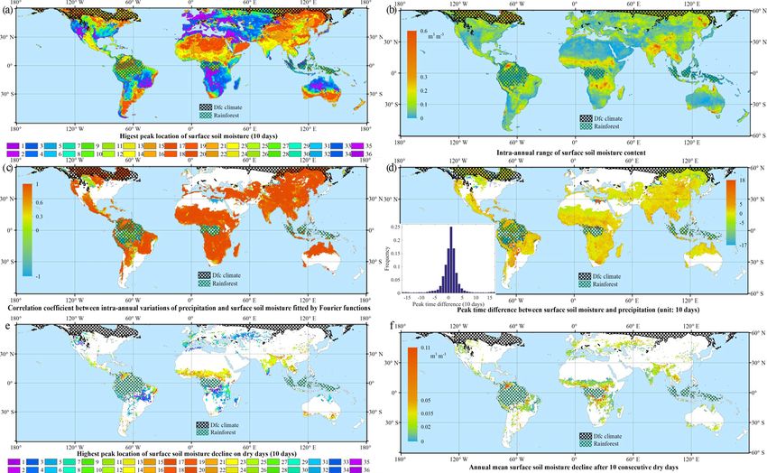
2                                                   Y. Chen et al.: An improved global RSSSM dataset covering 2003–2018

1   Introduction                                                  SMAP (Entekhabi et al., 2010), can produce significantly
                                                                  improved estimates because L-band microwaves (1.4 GHz;
Soil moisture plays an important role in modulating the ex-       Kerr et al., 2001) penetrate the vegetation canopy better than
change of water, carbon, and energy between the land sur-         shorter wavelengths (Burgin et al., 2017; Chen et al., 2018;
face and atmosphere, and it also links the global water, car-     Karthikeyan et al., 2017b; Kerr et al., 2016; Kim et al., 2018;
bon, and energy cycles (Dorigo et al., 2012; Karthikeyan et       Leroux et al., 2014a; Stillman and Zeng, 2018). However,
al., 2017a). Soil moisture has been endorsed by the Global        SMOS data are noisy and lack data in Eurasia due to high ra-
Climate Observing System (GCOS) as an essential climate           dio frequency interference (RFI) (Oliva et al., 2012). While
variable (Bojinski et al., 2014) because it can indicate the      the SMAP passive product has achieved an unbiased RMSE
climatic impact on the ecosystems, such as during ecological      that is close to its target of 0.04 m3 m−3 and has incorporated
droughts (Martínez-Fernández et al., 2016; Samaniego et al.,      hardware RFI mitigation (Chen et al., 2018; Colliander et al.,
2018). Current research requires high-quality soil moisture       2017), the data have only been available since March 2015.
information in terms of data accuracy and spatio-temporal            Interest in fusing satellite-observed and modelled soil
coverage (Hashimoto et al., 2015; Stocker et al., 2019).          moisture has increased recently. The European Space
   Reanalysis-based land surface model products are fre-          Agency (ESA) published a long-term surface soil moisture
quently used, including the Global Land Data Assimila-            dataset called the Climate Change Initiative (CCI), and the
tion System (GLDAS; with 0.25◦ resolution) (Rodell et al.,        latest version (v4.5) covers the time period of 1978–2018.
2004), European Reanalysis (ERA)-Interim (0.75◦ ) (Bal-           Two steps contribute to the combined CCI product. The first
samo et al., 2015), and its successors ERA5 (0.25◦ ) and          step involves rescaling the soil moisture of all microwave
ERA5-Land (0.1◦ ) (Hoffmann et al., 2019). These products         sensors against the reference data (GLDAS Noah product) by
can often predict temporal variations well due to the incor-      cumulative distribution function (CDF) matching, while the
poration of the time variance of environmental factors, e.g.      second step merges the rescaled products together by select-
precipitation. In addition, the modelling approach can also       ing the best product in each subperiod or averaging the prod-
provide information on the soil moisture in soil layers deeper    ucts weighted by the estimated errors (Dorigo et al., 2017;
than the surface layer (< 5 cm). The uncertainties arise from     Gruber et al., 2019; Liu et al., 2012). CCI utilized almost all
meteorological forcing data and model parameters as well as       the available microwave soil moisture datasets to form a long
inadequacies in model physics (Cheng et al., 2017). More-         time series and generally agrees well with measured values
over, the anthropogenic impacts from irrigation and land          at some sites, e.g. the Irish grassland sites and the grassland
cover changes are rarely considered (Kumar et al., 2015; Qiu      and agricultural fields in the United States, France, Spain,
et al., 2016).                                                    China, and Australia (Albergel et al., 2013; An et al., 2016;
   With advances of remote-sensing technology, microwave          Dorigo et al., 2017; Pratola et al., 2015). Valid microwave ob-
remote sensing became an alternative to soil moisture moni-       servations were quite limited before June 2002 due to satel-
toring. Currently, global-scale soil moisture can be acquired     lite sensor constraints (Dorigo et al., 2017). Through CDF
from either passive sensors (e.g. SMMR, SSM/I, TMI, Wind-         matching, the CCI soil moisture references the spatial pat-
Sat, AMSR-E, AMSR2, SMOS, SMAP; see Table 1 for the               terns of all the satellite products relative to that of GLDAS
full names) or active sensors (e.g. ERS and ASCAT), with          (Gruber et al., 2019; Liu et al., 2012, 2011b). The temporal
that within the top 5 cm of soil being detectable (Feng et al.,   variation in each satellite product is retained, although the
2017; Jiao et al., 2016; Piles et al., 2018). The data quality    data averaging (Liu et al., 2012) cannot efficiently distinguish
and spatial coverage are improved step by step (Karthikeyan       between the divergent interannual variations in various prod-
et al., 2017b). However, valid temporal spans of all these        ucts (Feng et al., 2017). The Soil Moisture Operational Prod-
sensors are limited, and the data quality and spatial cover-      uct System (SMOPS) v3.0 is another global blended surface
age were considered to be unsatisfactory until the launch of      soil moisture dataset that was developed in a similar way (Yin
AMSR-E in June 2002 (Karthikeyan et al., 2017b; Kawan-            et al., 2019). SMOPS v3.0 is a daily and 6-hourly temporal-
ishi et al., 2003). Currently, ASCAT sensors have produced        interval dataset with a complete global land coverage since
the longest continuous record of global surface soil mois-        March 2017. The overall performance, which is indicated
ture of microwave remote sensing (Bartalis et al., 2007), with    by an RMSE of 0.035–0.066 m3 m−3 is slightly lower than
the temporal span from 2007 until present. Satellite-based        that of CCI (with RMSE of 0.031–0.06 m3 m−3 ) (Wang et
soil moisture retrievals may also suffer from various distur-     al., 2021). The Global Land Evaporation Amsterdam Model
bances, such as lower quality over dense vegetation cover,        (GLEAM) surface soil moisture was produced by assimilat-
high open-water fractions, and complex topography (Draper         ing CCI data into a land surface model, GLEAM (Burgin et
et al., 2012; Fan et al., 2020; Ye et al., 2015). Differences     al., 2017; Martens et al., 2017; Miralles et al., 2011), through
in the algorithms dealing with the disturbances make dif-         an optimized Newtonian nudging approach (Martens et al.,
ferent microwave soil moisture products hardly compara-           2016). The general performance of the GLEAM soil mois-
ble with each other (Kim et al., 2015a; Mladenova et al.,         ture product is satisfactory (Beck et al., 2020). In the cur-
2014). New sensors, such as SMOS (Kerr et al., 2001) and          rent version, the CCI soil moisture anomalies (the deviations

Earth Syst. Sci. Data, 13, 1–31, 2021                                                 https://doi.org/10.5194/essd-13-1-2021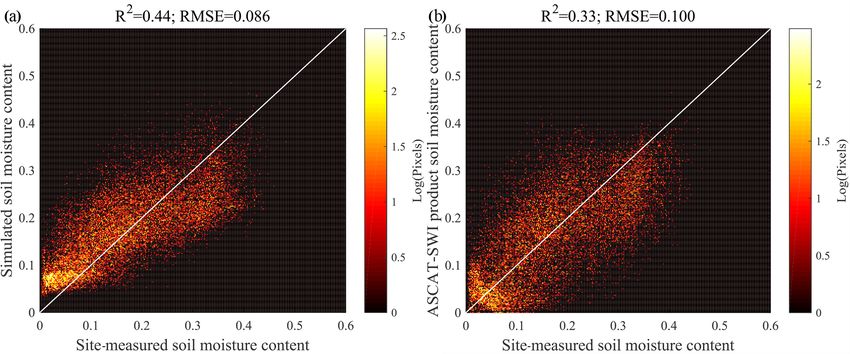
Y. Chen et al.: An improved global RSSSM dataset covering 2003–2018                                                                 3

Table 1. Abbreviations for the name of satellites, remote sensors, and missions.

                      Abbreviation     Full name
                      SMMR             Scanning Multichannel Microwave Radiometer
                      SSM/I            Special Sensor Microwave/Imager
                      TMI              Tropical Rainfall Measuring Mission (TRMM)’s Microwave Imager
                      AMSR-E           Advanced Microwave Scanning Radiometer for the Earth Observing System
                      AMSR2            Advanced Microwave Scanning Radiometer 2
                      SMOS             Soil Moisture Ocean Salinity
                      SMAP             Soil Moisture Active Passive
                      ERS              European Remote Sensing Active Microwave Instrument Wind Scatterometer
                      ASCAT            Advanced Scatterometer
                      MODIS            Moderate Resolution Imaging Spectroradiometer
                      MEaSUREs         Making Earth System Data Records for Use in Research Environments

to the seasonal climatology, which indicate whether the soil               A global long-term observational-based soil moisture
moisture at a time point is more humid or drier than the mul-           product was recently developed by building a neural network
tiyear average) are assimilated instead of the original CCI             between the SMOS product and the Tb data from AMSR-
time series (Martens et al., 2017). Therefore, satellite obser-         E (2003–September 2011) and AMSR2 (July 2012–2015)
vations play a much smaller role than modelling in form-                (Yao et al., 2017). Environmental factors, including the land
ing the GLEAM product. For further improvements in the                  surface temperature (LST) derived from the Tb at 36.5 GHz
efficiency of soil moisture assimilation, a high-quality long-          (Holmes et al., 2009) and the microwave vegetation index
term surface soil moisture dataset basically derived from mi-           (MVI; an indicator of vegetation cover), were also incorpo-
crowave remote sensing is highly needed.                                rated as ancillary inputs. The training R-squared value (R 2 )
   In addition to the CDF matching algorithm, at least four             of this product was only 0.45 (or correlation coefficient, r,
methods have been proposed that target the use of the in-               equals 0.67), and the validation against in situ measurements
formation acquired by one sensor to produce soil moisture               showed a temporal r of 0.52 and temporal RMSE of 0.084.
data that are compatible with the data retrieved from an-               Soil moisture data are partially missing due to the gap be-
other. Based on physically based equations (Wigneron et al.,            tween the temporal spans of AMSR-E and AMSR2 and the
2004), the regression between SMOS soil moisture and dual-              lack of SMOS data in Asia. As SMAP observations have be-
polarized brightness temperature (Tb ) data from AMSR-E is              come increasingly available, SMAP soil moisture data have
applied to match the AMSR-E soil moisture time series to                been chosen as the training target, thereby improving the
SMOS (R 2 = 0.36) (Al-Yaari et al., 2016). An example of                training R 2 to 0.55, while the overall r and RMSE against
the second method uses the Land Parameter Retrieval Model               measurements are 0.44 and 0.113 (Yao et al., 2019). An-
(LPRM) (Owe et al., 2008) to retrieve soil moisture from                other study rebuilt a soil moisture time series over the Ti-
SMOS and then match the “SMOS-LPRM” data with the                       betan Plateau by using SMAP data as the reference for a
AMSR-E-LPRM product by calibrating the LPRM param-                      random forest (Qu et al., 2019). For the environmental fac-
eters and then applying a linear regression (Van der Schalie            tors, while vegetation cover is not considered, elevation, In-
et al., 2017). Thirdly, copula functions allow us to model the          ternational Geosphere–Biosphere Programme (IGBP) land
structure of the dependence between two different Tb or soil            use cover type, grid location, and the day of a year (DOY)
moisture datasets and thus could perform better for the ex-             were chosen as ancillary inputs. The training R 2 in this re-
treme values, thereby reducing the RMSE (Gao et al., 2007;              gion reached 0.9, with a high temporal accuracy (temporal
Leroux et al., 2014b; Lorenz et al., 2018; Verhoest et al.,             r = 0.7; RMSE = 0.07 in the unfrozen season). However,
2015). To better characterize the nonlinear relationship be-            these data are regional (for the Tibetan Plateau only) and
tween two datasets (Rodriguez-Fernandez et al., 2015), re-              have a temporal gap between AMSR-E and AMSR2 data
searchers built a neural network that links SMOS soil mois-             (October 2011–June 2012).
ture to the Tb at different polarizations and frequencies of               Therefore, although previous studies have focused on
AMSR-E to produce a calibrated soil moisture data prod-                 developing long-term satellite-based surface soil moisture
uct that covers 9 years (2003–2011) (Rodríguez-Fernández                products using machine learning, major concerns remain to
et al., 2016). This approach proves to be efficient according           be addressed: (1) training designed for soil moisture estima-
to the connection between precipitation and the soil moisture           tion at the global scale should be more complex than that for
changes, as evaluated based on a data assimilation technique            only a specific region to ensure a satisfactory training effi-
and triple-collocation analysis results (Van der Schalie et al.,        ciency; (2) microwave observations are often limited to three
2018).                                                                  sensors, leading to temporal and spatial gaps at the global

https://doi.org/10.5194/essd-13-1-2021                                                       Earth Syst. Sci. Data, 13, 1–31, 2021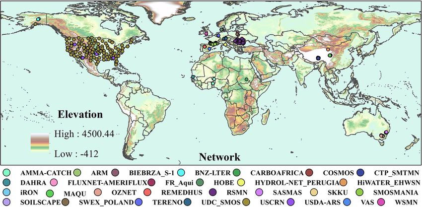
4                                                     Y. Chen et al.: An improved global RSSSM dataset covering 2003–2018

scale and limited training efficiency; (3) the environmental        cluded in the SMAP L4 Global Surface and Root Zone Soil
factors that should be incorporated as ancillary inputs have        Moisture Land Model Constants V004 dataset (hereinafter,
not been clarified. In this study, 11 high-quality microwave        “SMAP Constant”; note that porosity data were not provided
soil moisture products starting from 2003 are incorporated          in the ASCAT-SWI). Second, AMSR2-JAXA is the AMSR2
into iterative five-round neural networks to produce a spa-         soil moisture retrieved by the Japan Aerospace Exploration
tially and temporally continuous dataset for 2003–2018, and         Agency (JAXA) using Tb at the X band (10.65 GHz) (Fujii et
as many sources of microwave observational data as possible         al., 2009), and version 3 data on the Global Portal System
are used as predictors in each neural network. The quality          (G-Portal) were used. Third, AMSR2-LPRM-X stands for
impact factors of microwave soil moisture retrievals are also       the AMSR2 soil moisture produced by applying the LPRM
determined and then incorporated as ancillary inputs to im-         algorithm at the X band (Parinussa et al., 2014) (X-band re-
prove the training efficiency. Moreover, we designed local-         trievals may not perform well in high-vegetated areas, but C-
ized subnetworks instead of one global-scale neural network         band data such as AMSR2-LPRM-C or AMSR-E-LPRM-C
to account for the regional differences in training rules.          were not applied due to the high RFI, especially in the United
                                                                    States, Japan, and the Middle East; Njoku et al., 2005), and
                                                                    are obtained from NASA’s Earthdata Search website. The
2     Data and methods                                              fourth predictor, SMOS-IC (SMOS INRA-CESBIO), is a
                                                                    new SMOS soil moisture product created by INRA (Institut
2.1     Data for the production of global long-term surface         National de la Recherche Agronomique) and CESBIO (Cen-
        soil moisture data                                          tre d’Etudes Spatiales de la BIOsphère) with the main goal of
2.1.1    Satellite-based surface soil moisture data                 being as independent as possible from the auxiliary data, in-
         products                                                   cluding the simulated soil moisture (Fernandez-Moran et al.,
                                                                    2017a, b; Wigneron et al., 2007). The accuracy of SMOS-
SMAP currently has the highest quality of all remote-               IC has been proven to be higher than that of other SMOS
sensing-based soil moisture products (Al-Yaari et al., 2019)        products (Al-Yaari et al., 2019; Ma et al., 2019), and the data
and is thus chosen as the primary training target. The              version 105 offered by Centre Aval de Traitement des Don-
SMAP Enhanced L3 Radiometer Global Daily 9 km EASE-                 nées SMOS (CATDS) is adopted. TMI-LPRM-X is the X-
Grid Soil Moisture V002 (SPL3SMP_E_002; hereinafter                 band LPRM product of TMI and was created by the NASA
SMAP_E for short), which was developed by improving the             Goddard Space Flight Center (GSFC), which is used as the
spatial interpolation of the original 36 km resolution SMAP         5th predictor. Fengyun 3B is a Chinese meteorological satel-
soil moisture data (Chan et al., 2018), was adopted in this         lite with a Microwave Radiation Imager (MWRI) on board
study. SMAP_E was reprojected from the EASE-Grid 2.0                (Yang et al., 2011, 2012). The National Satellite Meteoro-
projection with 9 km resolution to the WGS 1984 geographic          logical Center product is retrieved using the Tb at 10.7 GHz,
coordinate system with 0.1◦ resolution. The nominal penetra-        and it is denoted by “FY-3B-NSMC” (the sixth predictor
tion depth of SMAP_E is ∼ 5 cm.                                     product). WindSat is onboard the Coriolis satellite (Gaiser
   Previous studies often used Tb observations at various           et al., 2004), and the soil moisture retrieved by LPRM at
bands as network inputs (Rodríguez-Fernández et al., 2016).         the X band (Parinussa et al., 2012) is provided by NASA
However, in this study, the well-acknowledged surface soil          (the seventh predictor). Three AMSR-E products are used,
moisture products retrieved through mature algorithms (see          including the NASA product (AE_Land3) created by the Na-
Fig. 1) are directly applied instead of Tb because (1) the pri-     tional Snow and Ice Data Center (AMSR-E-NSIDC) (Njoku
mary goal of this study is to calibrate and then fuse the exist-    et al., 2003), the JAXA product (AMSR-E-JAXA) (Fujii et
ing popular microwave soil moisture products, and (2) the Tb        al., 2009; Koike et al., 2004) obtained from G-Portal, and
signals at multiple bands contain too much information that         the LPRM product (AMSR-E-LPRM) available at the NASA
is not related to soil moisture, which may weaken the train-        Earthdata Search. All these data are reprojected to the WGS
ing efficiency and lead to overfitting. Although the drawback       1984 reference coordinate system and resampled to 0.1◦ .
is that the final soil moisture products may inherit the uncer-        To reduce noise and fill the gaps between sensor observa-
tainties associated with each retrieval method, this problem        tion tracks (at least 3 d are required for a microwave sensor
can be generally solved by including quality impact factors         to cover the whole globe), for every soil moisture product,
(see Sect. 2.1.2). The first satellite soil moisture product that   both the daytime and nighttime observations within each 10 d
is used as a predictor is the ASCAT soil water index (ASCAT-        period are combined by data averaging (the relative superi-
SWI) product, which was developed by the European Meteo-            ority of daytime and nighttime retrievals is not considered).
rological Satellite Organization (EUMETSAT) and provided            For example, for SMAP, 11 % of the global land surface has
by the ESA-Copernicus Land Monitoring Service (Albergel             data for only 5 d or less within a 10 d period. Therefore, the
et al., 2008; Wagner et al., 1999). The saturation degree in        temporal resolution of the dataset developed in this study is
the top soil layer (SWI_001) was converted to volumetric            approximately 10 d, meaning that three data records are ob-
soil moisture by multiplication with soil porosity data in-         tained within a month for days 1–10, 11–20, and from the

Earth Syst. Sci. Data, 13, 1–31, 2021                                                   https://doi.org/10.5194/essd-13-1-2021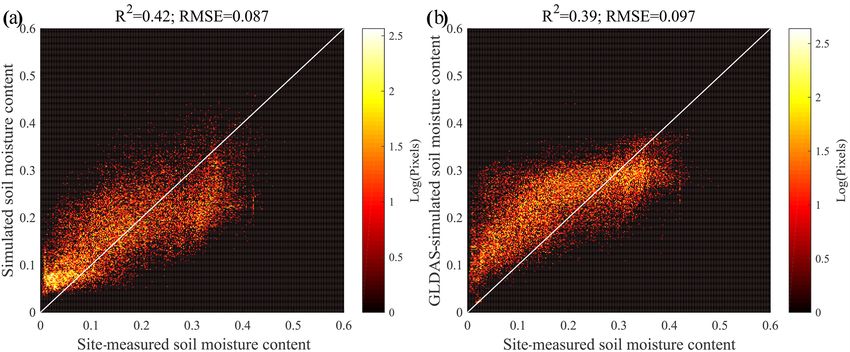
Y. Chen et al.: An improved global RSSSM dataset covering 2003–2018                                                                            5

Figure 1. Overview of the time periods of different soil moisture datasets and the “quality impact factor” products (e.g. leaf area index,
LAI, dataset) used in this study (listed above the timeline) as well as the periods of data applied for the training of the 67 independent neural
networks and the neural network simulation outputs (i.e. simulated soil moisture) in eight substeps (listed below the timeline).

https://doi.org/10.5194/essd-13-1-2021                                                             Earth Syst. Sci. Data, 13, 1–31, 2021
6                                                    Y. Chen et al.: An improved global RSSSM dataset covering 2003–2018

21st to the last day of that month. This format is exactly            Based on the two criteria above, the first environmental
the same as that of the ASCAT-SWI and many other prod-             factor to be included is the “vegetation factor” (i.e. vegetation
ucts developed by the Copernicus Land Monitoring Service           water content, VWC). Plants can absorb or scatter radiation
(https://land.copernicus.eu, last access: 19 September 2020).      from soil and emit radiation, thereby reducing the sensitivi-
                                                                   ties of both radiometers and radars to soil moisture (Du et al.,
                                                                   2000; Owe et al., 2001). However, L-band microwaves can
2.1.2   Quality impact factors of soil moisture retrievals         penetrate the vegetation layer better due to their longer wave-
                                                                   lengths (Konings et al., 2017; Piles et al., 2018). On the other
Environmental factors, including elevation, LST, and vege-         hand, although vegetation effects can be somewhat corrected
tation cover (indicated by the Normalized Difference Vege-         (Jackson and Schmugge, 1991), different methods have dif-
tation Index, MVI, etc.), were used as ancillary neural net-       ferent efficiencies. Radiative transfer models such as LPRM
work inputs to improve the soil moisture simulation (Lu et         may have difficulty describing the radiation attenuation by
al., 2015; Qu et al., 2019; Yao et al., 2017). According to        dense canopy due to the neglect of multiple scattering (Mo
these studies, these factors alone may not predict surface soil    et al., 1982; Owe et al., 2008), whereas the TU Wien change
moisture well without the incorporation of any microwave           detection algorithm applied to ASCAT utilizes the quadratic
remote-sensing data because although they are somewhat re-         polynomial dependence of backscatter on the incidence an-
lated to soil moisture (e.g. soil moisture is generally lim-       gle to better characterize the vegetation effect on backscat-
ited in areas with low vegetation cover but high in forests;       ter and then remove it by identifying the reference angles
McColl et al., 2017), the relationships are rather uncertain       (Hahn et al., 2017; Vreugdenhil et al., 2016). Microwave
(e.g. at smaller scales, the leaf area index (LAI) may have        vegetation indexes may contain large uncertainty and have
a negative influence on soil moisture due to the variation in      coarse resolutions (Liu et al., 2011a; Shi et al., 2008). The
evapotranspiration (Naithani et al., 2013) or may not have a       Normalized Difference Vegetation Index (NDVI) becomes
clear impact (Zhao et al., 2010); also, soil moisture can be       saturated at high vegetation cover (Huete et al., 2002). Be-
either high or low in summers, when vegetation peaks; Bal-         cause the LAI stands for the total leaf area per unit land,
docchi et al., 2006; Méndez-Barroso et al., 2009). However,        which is closely related to the VWC assuming a relatively
these factors are quite essential due to their direct impacts      stable leaf equivalent water thickness (Yilmaz et al., 2008),
on microwave-based soil moisture retrieval through the ra-         LAI is a suitable surrogate. Copernicus global 1 km reso-
diative transfer model and other models (Fan et al., 2020;         lution LAI (called GEOV2-LAI, which consists of SPOT-
Karthikeyan et al., 2017a); thus, they are retrieval-quality im-   VGT and PROBA-V LAI) data are adopted here due to the
pact factors. Detailed explanations are as follows. (1) The        high accuracy and full coverage (Baret et al., 2013; Cama-
bias of soil moisture estimates derived from a certain sen-        cho et al., 2013; Verger et al., 2014). Because the sensor con-
sor or a specific algorithm can be correlated with the degree      version from SPOT-VGT to PROBA-V in 2014 led to LAI
of disturbances from various environmental factors. For ex-        data discontinuity in specific areas (Cammalleri et al., 2019),
ample, in vegetated areas, LST is overestimated by LPRM            which may reduce neural network training and simulation ef-
(Ma et al., 2019), whereas soil moisture is underestimated by      ficiency, the Global LAnd Surface Satellite (GLASS) LAI
JAXA (Kim et al., 2015a), and the magnitudes of the biases         product (Xiao et al., 2014, 2016) from 2007–2017 is also
are often determined by vegetation amount or vegetation op-        used (Fig. 1). The LAIs are averaged on a monthly scale
tical depth (VOD). Therefore, the environmental factors are        and aggregated to 0.1◦ resolution. The second is the “wa-
essential for a better calibration of various products, espe-      ter fraction factor” (i.e. the fraction of water area in each
cially when soil moisture, which contains errors associated        pixel). Waters in land pixels dramatically decrease the Tb ,
with the retrieval method, is directly applied instead of the      thereby leading to overestimated soil moisture. Because dif-
Tb . (2) The relative performances of different products is also   ferent methods are used to detect and correct small areas of
controlled by environmental factors; for example, the AS-          water – either open water, wetlands, or partly inundated wet-
CAT product is preferable to AMSR-E-LPRM in vegetated              lands and croplands (Entekhabi et al., 2010; Kerr et al., 2001;
areas (Dorigo et al., 2010), while LST influences the relative     Mladenova et al., 2014; Njoku et al., 2003) – microwave soil
superiority of the LPRM and JAXA algorithms (Kim et al.,           moisture data calibration and weight assignment based on the
2015a). Therefore, for improved data fusion, the weights as-       water fraction within land pixels make sense (Ye et al., 2015).
signed to different soil moisture (or Tb ) predictor data avail-   In addition, the water fraction is a direct indicator of sur-
able at the same time should be determined by referring to         face soil moisture. In this study, the daily water area fraction
these quality impact factors (Kim et al., 2015b).                  derived from the Surface WAter Microwave Product Series
   In this study, nine quality impact factors are incorporated:    (SWAMPS) v3.2 dataset (Schroeder et al., 2015) is applied.
LAI, water fraction, LST, land use cover, tree cover frac-         The third factor is the “heat factor” (i.e. LST). Soil mois-
tion, non-tree vegetation fraction, topographic complexity,        ture retrievals from passive microwave sensors are based on
soil sand fraction, and clay fraction (see Fig. 1). The reasons    the correlation between the soil dielectric constant, which is
are as follows.                                                    influenced by soil moisture, and the emissivity estimated as

Earth Syst. Sci. Data, 13, 1–31, 2021                                                   https://doi.org/10.5194/essd-13-1-2021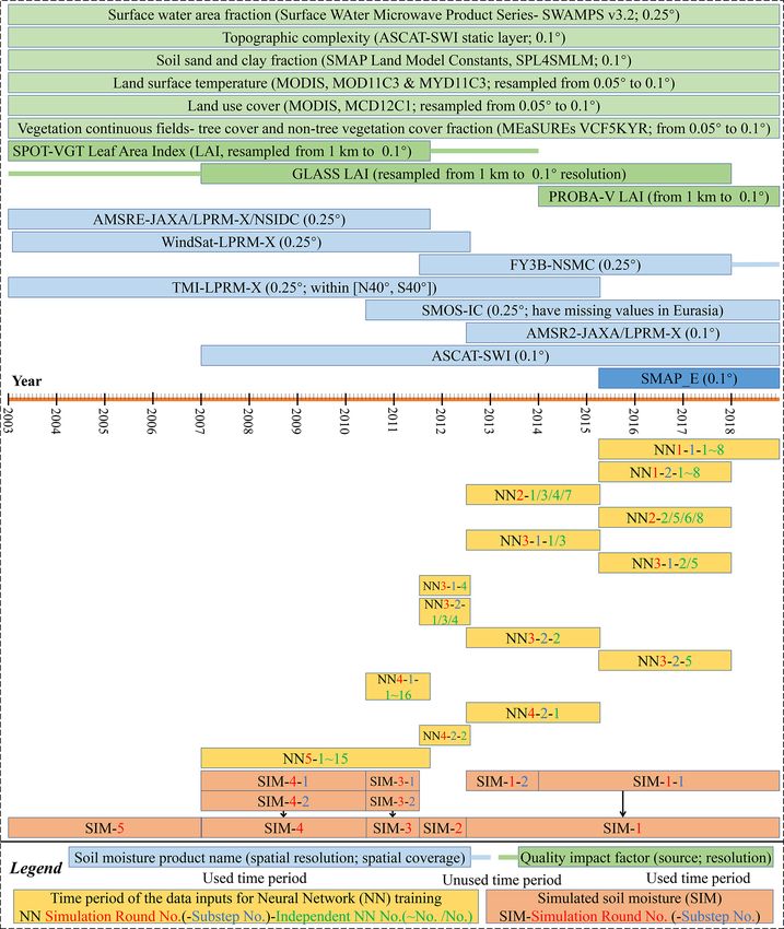
Y. Chen et al.: An improved global RSSSM dataset covering 2003–2018                                                              7

the ratio of Tb to soil physical temperature (Ts ) (Karthikeyan    calized neural networks (i.e. the rules for soil moisture pre-
et al., 2017a). Ts is approximate to the LST and can be de-        diction are separately trained in different 1◦ × 1◦ zones) fol-
rived from the Tb at 36.5 GHz (Holmes et al., 2009; Parinussa      lowed by surface soil moisture simulation based on the lo-
et al., 2011) or from reanalysis datasets including ECMWF,         calized neural networks; and (3) postprocessing, or the cor-
MERRA, and NCEP, or set as a constant of 293 K (Kim et             rection of potential errors or deficiencies in the soil moisture
al., 2015a). Active microwave products are independent of          simulation outputs.
LST (Ulaby et al., 1978). Because different LST estimates             The temporal span of the primary training target SMAP
are used in the retrievals of different soil moisture products,    does not overlap with that of TMI, FY-3B, WindSat, or
while the bias of each LST estimate compared to the actual         AMSR-E (see Fig. 1), while most microwave soil moisture
LST is influenced by the actual LST, we assume that the ac-        products are not available from the beginning year 2003 (e.g.
tual LST can determine the accuracy of every LST estimate          AMSR2 data are only available since July 2012). Therefore,
and finally the relative performances of various soil moisture     to fully utilize the 10 predictor surface soil moisture prod-
products (Kim et al., 2015a). In this study, we averaged the       ucts retrieved from seven different microwave sensors and
MODIS monthly LST acquired from the ascending and de-              form a temporally continuous soil moisture dataset covering
scending passes of both Terra and Aqua. Factors 4–6 are the        2003–2018, several iterative rounds of simulations are per-
“land cover factors”, which are added because the parameters       formed. Here, “iterative” means that the simulated soil mois-
essential for soil moisture retrieval (vegetation effect correc-   ture data in a round were also converted to part of the train-
tion) are set based on land use types (Griend and Wigneron,        ing targets of the next round’s neural network (hereinafter
2004; Jackson and Schmugge, 1991; Jackson et al., 1982;            the “secondary training targets”), thus extending the potential
Panciera et al., 2009). Additionally, landscape heterogeneity      temporal span of the target soil moisture data. Accordingly,
influences the retrieval accuracy (Lakhankar et al., 2009; Lei     the postprocessing steps which are intended to transform the
et al., 2018; Ma et al., 2019). Here, both the annual MODIS        simulation outputs to reliable secondary training targets can
land use cover maps and the MEaSUREs vegetation continu-           be seen as preprocessing steps as well. The basic flow of this
ous fields (i.e. the cover fractions of trees and non-tree vege-   process is shown in Fig. 2.
tation; Hansen and Song, 2018) are adopted. Apart from the
above dynamic factors, three (7th–9th) static factors are in-      2.2.1   Neural network design (1): localized neural
cluded: the “topographic factor” (i.e. topographic complex-                networks
ity) and the “soil texture factors” (two factors: sand fraction
and clay fraction) (Neill et al., 2011). Both factors can in-      In this study, instead of a universal network, we devised
fluence the relationship between soil moisture and emissivity      localized neural networks. The data within each individ-
or the dielectric constant (Dobson et al., 1985; Karthikeyan       ual zone are used to train a zonal neural network (here-
et al., 2017a; Njoku and Chan, 2006), but they are charac-         inafter a subnetwork), which is used for soil moisture
terized and corrected differently, leading to different relative   simulation at that zone. By comparison, localized neural
performances of various soil moisture products (Gao et al.,        networks help improve the training efficiency; however,
2006; Kim et al., 2015a). For topographic complexity, the          a smaller zonal size does not indicate a better simula-
static layer of the Copernicus ASCAT-SWI product (here-            tion accuracy. We noticed that over arid regions, the sur-
inafter the ASCAT Constant) is adopted, while for soil tex-        face soil moisture values retrieved by the LPRM algorithm
ture, the SMAP Constant is used (topographic complexity            (AMSR2/TMI/WindSat/AMSR-E-LPRM-X) can be obvi-
data are not available from SMAP Constant, while soil tex-         ously different on the two sides of each edge of 1◦ × 1◦ sized
ture is not provided by ASCAT Constant). The contribution          squares, which was probably attributed to the spatial distribu-
analysis results show that because various microwave soil          tion of key parameters (i.e. some parameters are at 1◦ resolu-
moisture retrievals have already been included, precipitation      tion). This finding suggests that subnetworks should be built
data are not an essential indicator of soil moisture and are not   at the 1◦ × 1◦ scale. Therefore, we divided the global extent
utilized as a physically based “quality impact factor” either      except the polar areas (80◦ N–60◦ S) into 140 × 360 zones.
(see Text S1 in the Supplement for detailed explanations).         Here, for a 0.1◦ pixel during a specific 10 d period, if all the
                                                                   input data (input soil moisture products and quality impact
2.2   Methods for the production of global long-term
                                                                   factors) have valid values, one valid data point is provided.
      surface soil moisture data
                                                                   Therefore, the maximal number of valid data points applied
                                                                   to train a subnetwork is 100 times the number of 10 d periods
Global long-term surface soil moisture data production in-         within the training period. The subnetworks with fewer than
cludes three basic parts, including (1) preprocessing, or the      100 valid data points (e.g. those in oceans) were dropped,
production of high-quality neural network inputs, including        leaving usually > 15 000 zonal subnetworks included in an
the training target soil moisture, predictor soil moisture prod-   independent neural network. The training was performed in
ucts, and the quality impact factors (i.e. nine environmental      MATLAB 2016a using the neural network fitting toolbox,
factors); (2) neural network operation, or the training of lo-     and the number of nodes in the hidden layer (between the

https://doi.org/10.5194/essd-13-1-2021                                                   Earth Syst. Sci. Data, 13, 1–31, 2021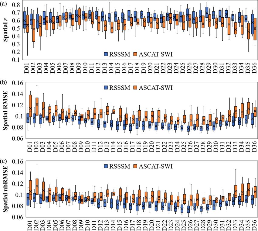
8                                                      Y. Chen et al.: An improved global RSSSM dataset covering 2003–2018

Figure 2. Flow chart for the production of global surface soil moisture data (remote-sensing-based surface soil moisture, RSSSM).

input and output layers; Stinchcombe and White, 1989) of               reported by ASCAT-SWI in most years, it should also be cov-
each subnetwork was seven. We chose the gradient descent               ered by snow or ice unless the thaw state is observed in the
backpropagation algorithm as the training function.                    MEaSUREs Global Record of Daily Landscape Freeze/Thaw
                                                                       Status V4 dataset. The simulated soil moisture in the rain-
2.2.2   Preprocessing and postprocessing steps                         forests identified in the “ASCAT Constant” is retained but
                                                                       not recommended due to the high uncertainty. On the other
After standardization of the original soil moisture data, to           hand, to avoid error propagation with the training times by
improve the neural network training efficiency, the potential          ensuring a high-quality training target for the next round’s
salt and pepper noises are removed. For each map (a specific           simulation, we remove all suspicious values for every simu-
10 d period), within each 1◦ × 1◦ zone, the soil moisture val-         lated result. This preprocessing step is performed by first ob-
ues are filtered to the level of 3 standard deviations relative        taining the maximal and minimum values of SMAP_E soil
to the mean in that zone (the principle is that 99.87 % of the         moisture in each pixel. If the simulated value is out of the
data appear within this range for a normal distribution (How-          range of the SMAP data during 2015–2018, then the value
ell et al., 1998); also note that the filter is applied spatially      is considered suspicious and not used as a training target.
rather than temporally to detect and delete the extreme val-           Subsequently, “3σ denoising” is performed again before the
ues, which are usually noise in mountain areas, and therefore          simulated soil moisture becomes a secondary training target,
the extreme climatic events will not be mistakenly removed).           which are referred to as SIM-1T, SIM-2T, and so on (“SIM”
This preprocessing step is thus called “3σ denoising”.                 stands for the simulated soil moisture, the number after the
   After neural network operation, boundary fuzzification is           hyphen indicates the round of simulation, and “T” means it
first applied, and it is a step in both preprocessing and post-        is applied as a training target; the temporal spans of SIM-XT
processing. Because the localized 1◦ × 1◦ network is applied           and SIM-X are the same, as shown in Fig. 1).
instead of the global network, the boundary between nearby
zones may be too obvious over some areas. To blur the
                                                                       2.2.3   Neural network design (2): five rounds of
boundary, a simple algorithm is applied as shown in Fig. S1
                                                                               simulations
in the Supplement. The soil moisture data with fuzzified
boundaries are transformed into both the final product and             The 11 microwave soil moisture data products with differ-
the next round’s training target. To produce the final prod-           ent temporal spans are incorporated and utilized as fully as
uct, two postprocessing steps are essential: filling of missing        possible through up to five rounds of neural-network-based
values and data masking. Because “3σ denoising” deleted                simulations, with at least four different soil moisture prod-
suspicious soil moisture retrievals, the simulation outputs            ucts retrieved from three different sensors applied as pre-
also contain few missing values, which can be simply filled            dictors in each round (see Fig. 1). Although increasing the
by sequentially searching and averaging nearby valid values            sources of soil moisture data inputs can improve the train-
(Chen et al., 2019). While the snow mask and ice mask of               ing efficiency, the spatial coverage of the simulation output
the ASCAT-SWI product can be transferred to the simulation             is sacrificed because the overlapping area decreases as the
output, the potential snow or ice cover before 2007 should be          number of soil moisture products increases. After all, most
identified. For a pixel in a specific 10 d period, if ice cover is     products have missing data in specific regions (e.g. moun-

Earth Syst. Sci. Data, 13, 1–31, 2021                                                       https://doi.org/10.5194/essd-13-1-2021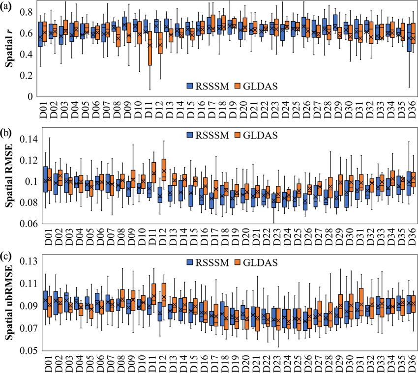
Y. Chen et al.: An improved global RSSSM dataset covering 2003–2018                                                               9

tains, wetlands, and urban settlements), and some sensors are       2012D19–2018, which is further divided into two parts:
even unable to produce data at the global scale (e.g. TMI           2014–2018 (substep 1), for which the PROBA-V LAI data
is limited to 40◦ N, 40◦ S; SMOS has many missing values            that begin in 2014 are applied, and 2012D19–2013 (sub-
in Eurasia). To resolve this dilemma, we classified all 0.1◦        step 2), for which GLASS LAI data are used (note: because
pixels according to the predictor soil moisture products that       GLASS LAI covers from the beginning of our study period
have a valid value over a 10 d period (for example, if there        until 2017, the training period for substep 2 is 2015D10–
are four predictor soil moisture datasets in one round, there       2017). The simulation results of the two substeps (SIM-1-1
should be 4 + 6 + 4 + 1 = 15 combinations; here, “1” indi-          and SIM-1-2) are combined as SIM-1, which is then trans-
cates the condition that all four products have a valid value       formed into a secondary training target, denoted as SIM-1T.
in the 0.1◦ pixel, and there are “6” conditions when only           In the second round of simulation, the training target can
two of the four predictors have a valid value in the pixel).        be either SMAP or SIM-1T, while the soil moisture input
However, to avoid soil moisture simulation under snow or            data are ASCAT, SMOS, TMI-LPRM-X (TMI), and FY-3B-
ice cover (see Sect. 2.2.2), not all combinations are consid-       NSMC (FY). The simulation output SIM-2 covers the pe-
ered. Then, an independent neural network corresponding to          riod of 2011D20–2012D18, which is constrained by the com-
each selected combination is trained. For data simulations          mon period of the four predictors (Tables S3–S4). SIM-2 was
in a 0.1◦ pixel, the most preferable independent neural net-        also converted into the training target SIM-2T. In the third
work is expected to be trained using all the available soil         round of neural network operation, the simulation period is
moisture data sources in that pixel (i.e. if valid values are       2010D16–2011D19. SMAP, SIM-1T, and SIM-2T are com-
provided by three soil moisture products, then the preferable       bined and used as the training targets (the training periods are
neural network is the one trained using those three predic-         within the range of 2011D20–2017D36), while the predictor
tors). However, in the 1◦ zone in which the 0.1◦ pixel is           soil moisture data are ASCAT, SMOS, TMI, and WindSat-
located, the subnetwork belonging to that preferable inde-          LPRM-X (WINDSAT). There are two substeps in round 3
pendent neural network may not exist due to limited valid           that are distinguished by whether the priority order of the
data points (see Sect. 2.2.1). Then, an alternative subnet-         neural networks is determined mainly based on the training
work driven by the combination of fewer soil moisture data          sample quantity and the training target quality (SIM-3-1) or
inputs should be applied instead. Hence, we should deter-           by first considering the number of predictor soil moisture
mine the neural network collocation that is the best choice         products (SIM-3-2; Tables S5–S8). Because these two meth-
for every pixel. Apart from applicability, the relative prior-      ods emphasize different aspects of neural network quality,
ity order of different neural networks was obtained by com-         in some pixels, SIM-3-1 will be advantageous, whereas in
prehensively considering the number and quality of input            others, SIM-3-2 could be better. Hence, an algorithm is de-
soil moisture products, the variety of sensors, the quantity        vised to combine the advantages of both simulations (SIM-
of training samples indicated by the number of 10 d peri-           3), which is described in Table S9. Next, the fourth round
ods, and the relative quality of the training targets (the train-   is for the simulations from 2007D01 to 2010D15. SIM-2T
ing target quality declines monotonically: SMAP > SIM-              and SIM-3T are combined to be the training target, and AS-
1T > SIM-2T > SIM-3T > SIM-4T). Occasionally, the two               CAT, WINDSAT, TMI, AMSR-E-JAXA, AMSR-E-LPRM-
most likely priority orders are given, and the simulation re-       X (AMSR-E-LPRM), and AMSR-E-NSIDC are all applied
sults of the corresponding two substeps are integrated later.       as predictors (LAI data now come from SPOT-VGT). Two
Specifically, when the LAI data source changes, the division        substeps are also considered. In the first substep, neural net-
of a single round into two substeps is also essential. Based on     works are sorted by focusing on the number of soil mois-
these principles, five rounds of neural networks are designed,      ture inputs and the sensors they are derived from, while the
with eight substeps containing a total of 67 independent neu-       training sample size and training target quality are priori-
ral networks. The training period for each neural network and       tized to create an alternative estimate (Tables S10–S13). Af-
the simulation period for each substep are shown in Fig. 1          terwards, SIM-4 is obtained by reasonably integrating these
(below the timeline), and the details are as follows.               two results. In the final round, the soil moisture simulation
   For the first round’s neural network (labelled as NN1),          is extended to as early as 2003. SIM-2T, SIM-3T, and SIM-
the potential training period is 2015D10–2018 (“D” is the           4T together are the training targets, while the predictor soil
ordinal of the 10 d period; therefore, “2015D10” represents         moisture data entering the neural networks consist of WIND-
the period from 1 April to 10 April 2015) because SMAP              SAT, TMI, AMSR-E-JAXA, AMSR-E-LPRM, and AMSR-
soil moisture data that cover only that period are applied          E-NSIDC (Tables S14–S15).
as the training target, while ASCAT-SWI10 (abbreviated as
ASCAT), SMOS-IC (SMOS), AMSR2-JAXA, and AMSR2-                      2.3   Methods for the validation of surface soil moisture
LPRM-X (AMSR2-LPRM) are the four soil moisture prod-                      products
ucts used as predictors (details are in Tables S1–S2 in the
Supplement). Because all four predictors have data since            For the evaluation of global-scale soil moisture data, we
2012D19, the potential soil moisture simulation period is           adopted the International Soil Moisture Network (ISMN)

https://doi.org/10.5194/essd-13-1-2021                                                    Earth Syst. Sci. Data, 13, 1–31, 2021
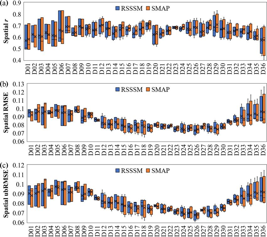
10                                                     Y. Chen et al.: An improved global RSSSM dataset covering 2003–2018

Figure 3. Global distribution of the networks and stations in the ISMN dataset.

dataset (Dorigo et al., 2011, 2013). Because the training               record of satellite-based soil moisture (ASCAT-SWI; con-
target SMAP represents the soil moisture within 0–5 cm,                 verted to volumetric fraction; data period is 2007–2018),
the simulated soil moisture is intended for that surface soil           the reanalysis-based soil moisture (GLDAS Noah V2.1
layer as well. Accordingly, the measurements used for val-              and ERA5-Land; data were resampled, 10 d averaged and
idation are limited to ≤ 5 cm depth. Records outside of the             then evaluated during 2003–2018), and the soil moisture
RSSSM data period (2003–2018), such as those from Rus-                  datasets developed by combining both satellite observations
sian networks, are ignored as well. The quality flags of                and model simulations (CCI v4.5 and GLEAM v3.3; for
ISMN (Dorigo et al., 2013) are also checked to retain only              v3.3a, the radiation and air temperature forcing data come
the “good-quality” data. After data screening and process-              from ERA5, whereas for v3.3b, all meteorological data
ing (e.g. the pixels with average annual maximal water area             are satellite-based, yet the data after September 2018 are
fractions greater than 5 % are excluded, please see Text S2),           not available). The overall performance of any soil mois-
more than 100 000 ∼ 10 d averaged soil moisture records ob-             ture product is first evaluated using all of the validation
tained from 728 stations of 29 networks are applied for vali-           datasets, with Pearson R-squared (R 2 ) and RMSE values
dation of the soil moisture products. The detailed information          (unit: m3 m−3 ) adopted as the main indicators. The next step
of these stations and the periods of the data used are listed in        is temporal-pattern validation. For pixels with enough (> 20)
Table S16, while the spatial distribution of these stations is          10 d averaged in situ records, we compare the estimated
shown in Fig. 3. The major climate types of the sites are de-           soil moisture during all periods against the corresponding
termined from the Köppen–Geiger climate classification map              measurements and calculate the Pearson correlation coef-
(see Table 2 for the description; Kottek et al., 2006). Next,           ficient (r) and RMSE. Several supplementary indexes are
we further aggregated the site-scale 10 d averaged soil mois-           also added, including bias, unbiased RMSE (ubRMSE), and
ture data to a 0.1◦ pixel scale by averaging all the measure-           the correlation coefficient between the anomalies (anoma-
ments made by different stations or different sensors within            lies r, abbreviated here as “A.R”; A.R can better indicate
the pixel (Gruber et al., 2020). Specifically, if soil moisture is      the simulation accuracy of interannual variations; soil mois-
not simulated due to snow or ice cover, then the correspond-            ture anomalies are calculated by Eq. 1). Next, we compare
ing measurement is useless. This process resulted in a final            the means and medians of the above evaluation indexes for
collection of ∼ 40 000 pixel-scale 10 d period soil moisture            different soil moisture products and test whether the differ-
records within the validation dataset.                                  ences are significant. Moreover, the relative performances of
   The soil moisture datasets to be evaluated include the               various products in different climatic zones are analysed. Fi-
RSSSM product in this study (remote-sensing-based sur-                  nally, we perform spatial-pattern validation. In detail, for ev-
face soil moisture, covering 2003–2018), SMAP_E (the pri-               ery 10 d period, we compare all the soil moisture measure-
mary training target, covering April 2015–2018), the longest            ments that are upscaled to 0.1◦ during that period with the

Earth Syst. Sci. Data, 13, 1–31, 2021                                                       https://doi.org/10.5194/essd-13-1-2021
Y. Chen et al.: An improved global RSSSM dataset covering 2003–2018                                                                  11

Table 2. Description of the Köppen–Geiger climate classification types at all the selected ISMN stations.

                                 Climate_Köppen    General description
                                 Aw                Equatorial savannah with dry winter
                                 BSk               Steppe climate, cold and arid
                                 BWh               Desert climate, hot and arid
                                 BWk               Desert climate, cold and arid
                                 Cfa               Warm temperate climate, fully humid, hot summer
                                 Cfb               Warm temperate climate, fully humid, warm summer
                                 Csa               Warm temperate climate with dry, hot summer
                                 Csb               Warm temperate climate with dry, warm summer
                                 Dfa               Snow climate, fully humid, hot summer
                                 Dfb               Snow climate, fully humid, warm summer
                                 Dfc               Snow climate, fully humid, cool summer and cold winter
                                 Dsb               Snow climate with dry, warm summer
                                 Dwc               Snow climate with cool summer and cold, dry winter
                                 ET                Tundra climate

corresponding estimated values. The spatial-pattern evalua-              2.4   Methods for the intra-annual variation analysis of
tion indexes include the correlation coefficient (r), RMSE,                    surface soil moisture
bias, and ubRMSE values (Eq. 2). The relative superiority of
all products during different 10 d periods in a year and the
                                                                         Because the original resolution of SMAP soil moisture is
changes in data coverage as well as data quality with time
                                                                         ∼ 0.4◦ , while that of most predictor soil moisture products is
are also investigated.
                                                                         0.25◦ , the intra-annual variation analysis of RSSSM is per-
             ny                                                          formed at 0.5◦ resolution. We also exclude high-latitude ar-
                                                                         eas (60–90◦ N) where the available data are limited due to
             P
                  SSM (y, k)
            y=1                                                         frequent ice cover. Fourier functions can characterize intra-
SSM (k) =                       ny ≥ 3
                    ny                                                   annual variation well (Brooks et al., 2012; Hermance et
                                                                         al., 2007). Therefore, for the remaining areas (60◦ S–60◦ N),
SSM is either estimated or measured. SSM is surface soil                 based on a total of 36×16 (years) = 576 data points, we fit the
moisture, k is the ordinal of a 10 d period in a year, y is a            intra-annual cycle of soil moisture using the Fourier function,
year with measured SSM in the kth 10 d period, and ny is the             with the period fixed to 1 year (36 10 d periods). The num-
number of those years.                                                   ber of terms is set to 1 unless the intra-annual cycle is obvi-
                                                                         ously asymmetrical and can be much better characterized by
SSManom (y, k) = SSM (y, k) − SSM(t),                          (1)       a two-term Fourier function. Subsequently, the highest peak
                                                                         and lowest trough values of surface soil moisture as well as
where SSManom (y, t) is the anomalies of surface soil mois-
                                                                         the corresponding locations in time (the ordinal of 10 d) are
ture during the tth 10 d period in year y (Eq. 1).
                                                                         exported.
            Png                                                             The direct driving factor of the variation in surface
              i=1 SSMest,i                                               soil moisture is precipitation, for which we adopted the
SSMest =
                   ng                                                    GPM (Global Precipitation Measurement) IMERG (Inte-
            Png                                                          grated Multi-satellitE Retrievals for GPM) Precipitation V06
              i=1 SSMact,i

SSMact =                        ng ≥ 20 ,                                Final Run data (Huffman et al., 2019). Apart from a direct
                   ng
                                                                         correlation analysis, we also explored the relationship be-
where i is a grid with upscaled surface soil moisture mea-               tween the intra-annual cycles of precipitation and surface soil
surements during a specific 10 d period, and ng is the number            moisture using Fourier fitting (the derived fitting function is
of those grids on the globe.                                             dropped if the adjusted R 2 is lower than 0.1), with the peak
                                                                         time difference in each 0.5◦ grid cell calculated (if both cy-
ubRMSEspatial                                                            cles have two peaks, the average locations of the two peaks
  v                                                                      are calculated). Because RSSSM indicates the average soil
  u ng                                                                   moisture condition during every 10 d period, we evaluate the
  uX
= t [ SSM         est,i   − SSMest − SSMest,i − SSMact ]2 /ng            surface soil moisture decline after 20 consecutive days (i.e.
      i=1                                                                two adjacent 10 d periods) without effective precipitation to
                                                               (2)       explore the impact of dry periods on surface soil moisture.

https://doi.org/10.5194/essd-13-1-2021                                                          Earth Syst. Sci. Data, 13, 1–31, 2021
12 Y. Chen et al.: An improved global RSSSM dataset covering 2003–2018
Effective precipitation is calculated by precipitation minus Next, we compare the spatial accuracy of RSSSM and
canopy interception, which is estimated by the modified Mer- SMAP. The spatial correlation of RSSSM is somewhat re-
riam canopy interception model (Kozak et al., 2010; Mer- duced compared to the training target, while the RMSE is
riam, 1960). If the total effective precipitation within two slightly increased (Table 4), indicating a subtle loss of de-
consecutive 10 d periods (20 d) is less than a given thresh- tailed spatial information through neural network operation.
old (initially set to 10 mm), we consider the soil moisture Because ISMN stations are mostly located in the middle to
change in the latter period compared to the previous period high latitudes of the Northern Hemisphere, Fig. 6 shows that
to be mostly due to surface evaporation and percolation (cap- (1) the accuracy of RSSSM is highest in summers (growing
illary rise is negligible; McColl et al., 2017); thus, it should seasons) and lowest in winters, which is inherited from its
be negative. Hence, for a 0.5◦ grid cell, if the number of neg- origin (SMAP), probably due to the impact of freezing on
ative values does not meet 2 times the number of positive soil moisture retrieval, and (2) RSSSM has a similar spatial
values, the precipitation threshold is reduced by 1 mm until accuracy as SMAP in most periods except for May to June
that condition is satisfied. This loop is terminated when there and November to December.
are fewer than 36 available data points in dry periods (the
maximal number of data points is 576), and then the grid cell 3.2 Accuracy comparison between RSSSM and popular
is excluded from the analysis. In desert areas, the random global long-term soil moisture products
noise of the surface soil moisture product can hide the sig-
nal of moisture changes, while in wet areas (e.g. rainforests), 3.2.1 Data quality comparison between RSSSM and the
20 d without effective precipitation seldom occurs, thus lead- satellite-derived product
ing to no results over most areas. In the remaining areas, the The satellite-derived global surface soil moisture product
intra-annual variation in the surface soil moisture loss during ASCAT-SWI now covers 12 years, 2007–2018. During that
dry days can be fitted by the Fourier function as well, which period, the overall R 2 and RMSE for RSSSM are 0.44 and
is then analysed using the above methods. 0.086, respectively (Fig. 7), which appear to be much better
than those for ASCAT-SWI (R 2 = 0.33, RMSE = 0.100). If
3 Results the data period of SMAP (2015D10–2018) is excluded, the
overall R 2 and RMSE for RSSSM are 0.43 and 0.087, re-
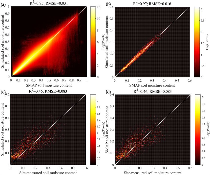
3.1 Neural network training efficiency: a comparison spectively, which are still better than those for ASCAT-SWI
between RSSSM and SMAP (R 2 = 0.33, RMSE = 0.1). However, RSSSM overestimates
soil moisture when low moisture occurs, which is a problem
To examine the training and simulation efficiency of the neu-
inherited from the SMAP product (Fig. 4), and is a bit non-
ral network, we compare the neural-network-simulated sur-
linearly correlated with the measured values (Fig. 7a).
face soil moisture (RSSSM) with the training target SMAP
According to the temporal-validation results (Table 3), the
(note: these two datasets are not completely independent
evaluation indexes, including r, RMSE, bias, and ubRMSE,
because SMAP data are used as the training target, while
are all significantly (p < 0.05) better for RSSSM than
RSSSM data are the simulation results) during April 2015–
ASCAT-SWI (anomalies r for RSSSM are also higher but
2018. The R 2 reaches up to 0.95, while the RMSE is
not significant). The temporal accuracy of RSSSM appears
0.031 m3 m−3 ) (Fig. 4a). If only the pixels with measured
to be obviously higher in all climatic zones except for polar
data are considered, the consistency between RSSSM and
areas (Dsb, Dwc, and ET). Specifically, in arid areas (BWh
SMAP becomes even stronger, with an R 2 of 0.97 and an
and BWk), the temporal-correlation coefficients for ASCAT-
RMSE of 0.016 (Fig. 4b). When validated against site mea-
SWI are much lower and even negative (Fig. 8). This prob-
surements, the R 2 and RMSE values are 0.46 and 0.083, re-
lem is known and might be related to the different scattering
spectively, for both RSSSM and SMAP (Fig. 4c and d). All
mechanisms in dry soils, invalidating the assumptions of the
these findings justify the high training and prediction effi-
change detection method (Al-Yaari et al., 2014).
ciency of the neural network set designed in this study.
The spatial accuracy of RSSSM is found to be signifi-
According to Table 3, RSSSM is just slightly lower than
cantly higher than that of ASCAT-SWI when any evaluation
SMAP in terms of temporal accuracy (the differences in the
index is considered (Table 4). Moreover, the results show that
five indicators – r, RMSE, bias, ubRMSE, and A.R – are all
RSSSM is generally superior to ASCAT-SWI throughout the
nonsignificant). Figure 5 indicates generally the same level of
year, especially during the growing seasons (Fig. 9).
temporal accuracy for RSSSM and SMAP under all climates.
RSSSM cannot adequately characterize the temporal varia-
tion in soil moisture in the “Dfc” (snow climate, fully humid; 3.2.2 Data quality comparison between RSSSM and
see Table 2) region because the training target, SMAP, does land surface model products
not have a high temporal accuracy in this area, probably due First, the overall accuracies of RSSSM and GLDAS Noah
to frequent freezing and melting processes. V2.1 surface soil moisture data from 2003 to 2018 are com-
pared. While RSSSM is nonlinearly correlated with mea-
Earth Syst. Sci. Data, 13, 1–31, 2021 https://doi.org/10.5194/essd-13-1-2021You can also read