MLAir (v1.0) - a tool to enable fast and flexible machine learning on air data time series - GMD
←
→
Page content transcription
If your browser does not render page correctly, please read the page content below
Geosci. Model Dev., 14, 1553–1574, 2021
https://doi.org/10.5194/gmd-14-1553-2021
© Author(s) 2021. This work is distributed under
the Creative Commons Attribution 4.0 License.

MLAir (v1.0) – a tool to enable fast and flexible
machine learning on air data time series
Lukas Hubert Leufen1,2 , Felix Kleinert1,2 , and Martin G. Schultz1
1 Jülich   Supercomputing Centre, Research Centre Jülich, Jülich, Germany
2 Institute  of Geosciences, Rhenish Friedrich Wilhelm University of Bonn, Bonn, Germany

Correspondence: Lukas Hubert Leufen (l.leufen@fz-juelich.de)

Received: 9 October 2020 – Discussion started: 23 October 2020
Revised: 29 January 2021 – Accepted: 2 February 2021 – Published: 17 March 2021

Abstract. With MLAir (Machine Learning on Air data) we             1   Introduction
created a software environment that simplifies and acceler-
ates the exploration of new machine learning (ML) models,
specifically shallow and deep neural networks, for the anal-       In times of rising awareness of air quality and climate is-
ysis and forecasting of meteorological and air quality time        sues, the investigation of air quality and weather phenomena
series. Thereby MLAir is not developed as an abstract work-        is moving into focus. Trace substances such as ozone, nitro-
flow, but hand in hand with actual scientific questions. It thus   gen oxides, or particulate matter pose a serious health haz-
addresses scientists with either a meteorological or an ML         ard to humans, animals, and nature (Cohen et al., 2005; Ben-
background. Due to their relative ease of use and spectacular      tayeb et al., 2015; World Health Organization, 2013; Lefohn
results in other application areas, neural networks and other      et al., 2018; Mills et al., 2018; US Environmental Protec-
ML methods are also gaining enormous momentum in the               tion Agency, 2020). Accordingly, the analysis and prediction
weather and air quality research communities. Even though          of air quality are of great importance in order to be able to
there are already many books and tutorials describing how to       initiate appropriate countermeasures or issue warnings. The
conduct an ML experiment, there are many stumbling blocks          prediction of weather and air quality has been established op-
for a newcomer. In contrast, people familiar with ML con-          erationally in many countries and has become a multi-million
cepts and technology often have difficulties understanding         dollar industry, creating and selling specialized data products
the nature of atmospheric data. With MLAir we have ad-             for many different target groups.
dressed a number of these pitfalls so that it becomes easier          These days, forecasts of weather and air quality are gener-
for scientists of both domains to rapidly start off their ML       ally made with the help of so-called Eulerian grid point mod-
application. MLAir has been developed in such a way that it        els. This type of model, which solves physical and chemical
is easy to use and is designed from the very beginning as a        equations, operates on grid structures. In fact, however, lo-
stand-alone, fully functional experiment. Due to its flexible,     cal observations of weather and air quality are strongly in-
modular code base, code modifications are easy and personal        fluenced by the immediate environment. Such local influ-
experiment schedules can be quickly derived. The package           ences are quite difficult for atmospheric chemistry models
also includes a set of validation tools to facilitate the evalu-   to accurately simulate due to the limited grid resolution of
ation of ML results using standard meteorological statistics.      these models and because of uncertainties in model parame-
MLAir can easily be ported onto different computing envi-          terizations. Consequently, both global models and so-called
ronments from desktop workstations to high-end supercom-           small-scale models, whose grid resolution is still in the mag-
puters with or without graphics processing units (GPUs).           nitude of about a kilometre and thus rather coarse in compar-
                                                                   ison to local-scale phenomena in the vicinity of a measure-
                                                                   ment site, show a high uncertainty of the results (see Vautard,
                                                                   2012; Brunner et al., 2015). To enhance the model output,
                                                                   approaches focusing on the individual point measurements

Published by Copernicus Publications on behalf of the European Geosciences Union.
1554 L. H. Leufen et al.: MLAir (v1.0) at weather and air quality monitoring stations through down- of graphics processing units (GPUs) due to the underlying scaling methods are applied allowing local effects to be taken ML library. MLAir is suitable for ML beginners due to its into account. Unfortunately, these methods, being optimized simple usage but also offers high customization potential for for specific locations, cannot be generalized for other regions advanced ML users. It can therefore be employed in real- and need to be re-trained for each measurement site. world applications. For example, more complex model archi- Recently, a variety of machine learning (ML) methods tectures can be easily integrated. ML experts who want to ex- have been developed to complement the traditional down- plore weather or air quality data will find MLAir helpful as it scaling techniques. Such methods (e.g. neural networks, ran- enforces certain standards of the meteorological community. dom forest) are able to recognize and reproduce underly- For example, its data preparation step acknowledges the au- ing and complex relationships in data sets. Driven in par- tocorrelation which is typically seen in meteorological time ticular by computer vision and speech recognition, tech- series, and its validation package reports well-established nologies like convolutional neural networks (CNNs; Lecun skill scores, i.e. improvement of the forecast compared to ref- et al., 1998), or recurrent networks variations such as long erence models such as persistence and climatology. From a short-term memory (LSTM; Hochreiter and Schmidhuber, software design perspective, MLAir has been developed ac- 1997) or gated recurrent units (GRUs; Cho et al., 2014) but cording to state-of-the-art software development practices. also more advanced concepts like variational autoencoders This article is structured as follows. Section 2 introduces (VAEs; Kingma and Welling, 2014; Rezende et al., 2014), or MLAir by expounding the general design behind the MLAir generative adversarial networks (GANs; Goodfellow et al., workflow. We also share a few more general points about 2014), are powerful and widely and successfully used. The ML and what a typical workflow looks like. This is followed application of such methods to weather and air quality data by Sect. 3 showing three application examples to allow the is rapidly gaining momentum. reader to get a general understanding of the tool. Further- Although the scientific areas of ML and atmospheric sci- more, we show how the results of an experiment conducted ence have existed for many years, combining both disciplines by MLAir are structured and which statistical analysis is ap- is still a formidable challenge, because scientists from these plied. Section 4 extends further into the configuration options areas do not speak the same language. Atmospheric scientists of an experiment and details on customization. Section 5 de- are used to building models on the basis of physical equations lineates the limitations of MLAir and discusses for which and empirical relationships from field experiments, and they applications the tool might not be suitable. Finally, Sect. 6 evaluate their models with data. In contrast, data scientists concludes with an overview and outlook on planned devel- use data to build their models on and evaluate them either opments for the future. with additional independent data or physical constraints. This At this point we would like to point out that in order to elementary difference can lead to misinterpretation of study simplify the readability of the paper, highlighting is used. results so that, for example, the ability of the network to gen- Frameworks are highlighted in italics and typewriter font is eralize is misjudged. Another problem of several published used for code elements such as class names or variables. studies on ML approaches to weather forecasting is an in- Other expressions that, for example, describe a class but do complete reporting of ML parameters, hyperparameters, and not explicitly name it, are not highlighted at all in the text. data preparation steps that are key to comprehending and re- Last but not least, we would like to mention that MLAir is an producing the work that was done. As shown by Musgrave open-source project and contributions from all communities et al. (2020) these issues are not limited to meteorological are welcome. applications of ML only. To further advance the application of ML in atmospheric science, easily accessible solutions to run and document ML 2 MLAir workflow and design experiments together with readily available and fully docu- mented benchmark data sets are urgently needed (see Schultz ML in general is the application of a learning algorithm to et al., 2021). Such solutions need to be understandable by a data set whereby a statistical model describing relations both communities and help both sides to prevent unconscious within the data is generated. During the so-called training blunders. A well-designed workflow embedded in a meteo- process, the model learns patterns in the data set with the rological and ML-related environment while accomplishing aid of the learning algorithm. Afterwards, this model can be subject-specific requirements will bring forward the usage of applied to new data. Since there is a large number of learning ML in this specific research area. algorithms and also an arbitrarily large number of different In this paper, we present a new framework to enable ML architectures, it is generally not possible to determine in fast and flexible Machine Learning on Air data time series advance which approach will deliver the best results under (MLAir). Fast means that MLAir is distributed as full end- which configuration. Therefore, the optimal setting must be to-end framework and thereby simple to deploy. It also al- found by trial and error. lows typical optimization techniques to be deployed in ML ML experiments usually follow similar patterns. First, data workflows and offers further technical features like the use must be obtained, cleaned if necessary, and finally put into a Geosci. Model Dev., 14, 1553–1574, 2021 https://doi.org/10.5194/gmd-14-1553-2021
L. H. Leufen et al.: MLAir (v1.0)                                                                                             1555

suitable format (preprocessing). Next, an ML model is se-              Concerning the ML framework, Keras (Chollet et al.,
lected and configured (model setup). Then the learning algo-        2015, release 2.2.4) was chosen for the ML parts using Ten-
rithm can optimize the model under the selected settings on         sorFlow (release 1.13.1) as back-end. Keras is a framework
the data. This optimization is an iterative procedure and each      that abstracts functionality out of its back-end by providing a
iteration is called an epoch (training). The accuracy of the        simpler syntax and implementation. For advanced model ar-
model is then evaluated (validation). If the results are not sat-   chitectures and features it is still possible to implement parts
isfactory, the experiment is continued with modified settings       or even the entire model in native TensorFlow and use the
(i.e. hyperparameters) or started again with a new model. For       Keras front-end for training. Furthermore, TensorFlow has
further details on ML, we refer to Bishop (2006) and Good-          GPU support for training acceleration if a GPU device is
fellow et al. (2016) but would also like to point out that there    available on the running system.
is a large amount of further introductory literature and freely        For data handling, we chose a combination of xar-
available blog entries and videos, and that the books men-          ray (Hoyer and Hamman, 2017; Hoyer et al., 2020, re-
tioned here are only two of many options out there.                 lease 0.15.0) and pandas (Wes McKinney, 2010; Reback
   The overall goal of designing MLAir was to create a ready-       et al., 2020, release 1.0.1). pandas is an open-source tool
to-run ML application for the task of forecasting weather           to analyse and manipulate data primarily designed for tab-
and air quality time series. The tool should allow many cus-        ular data. xarray was inspired by pandas and has been devel-
tomization options to enable users to easily create a custom        oped to work with multi-dimensional arrays as simply and
ML workflow, while at the same time it should support users         efficiently as possible. xarray is based on the off-the-shelf
in executing ML experiments properly and evaluate their re-         Python package for scientific computing NumPy (van der
sults according to accepted standards of the meteorological         Walt et al., 2011, release 1.18.1) and introduces labels in the
community. At this point, it is pertinent to recall that MLAir’s    form of dimensions, coordinates, and attributes on top of raw
current focus is on neural networks.                                NumPy-like arrays.
   In this section we present the general concepts on which
MLAir is based. We first comment on the choice of the un-           2.2   Design of the MLAir workflow
derlying programming language and the packages and frame-
works used (Sect. 2.1). We then focus on the design consid-         According to the goals outlined above, MLAir was designed
erations and choices and introduce the general workflow of          as an end-to-end workflow comprising all required steps of
MLAir (Sect. 2.2). Thereafter we explain how the concepts           the time series forecasting task. The workflow of MLAir is
of run modules (Sect. 2.3), model class (Sect. 2.4), and data       controlled by a run environment, which provides a central
handler (Sect. 2.5) were conceived and how these modules            data store, performs logging, and ensures the orderly exe-
interact with each other. More detailed information on, for         cution of a sequence of individual stages. Different work-
example, how to adapt these modules can be found in the             flows can be defined and executed under the umbrella of this
corresponding subsection of the later Sect. 4.                      environment. The standard MLAir workflow (described in
                                                                    Sect. 2.3) contains a sequence of typical steps for ML exper-
2.1   Coding language                                               iments (Fig. 1), i.e. experiment setup, preprocessing, model
                                                                    setup, training, and postprocessing.
Python (Python Software Foundation, 2018, release 3.6.8)               Besides the run environment, the experiment setup plays
was used as the underlying coding language for several rea-         a very important role. During experiment setup, all cus-
sons. Python is pretty much independent of the operating sys-       tomization and configuration modules, like the model class
tem and code does not need to be compiled before a run.             (Sect. 2.4), data handler (Sect. 2.5), or hyperparameters, are
Python is flexible to handle different tasks like data load-        collected and made available to MLAir. Later, during execu-
ing from the web, training of the ML model or plotting.             tion of the workflow, these modules are then queried. For ex-
Numerical operations can be executed quite efficiently due          ample, the hyperparameters are used in training whereas the
to the fact that they are usually performed by highly op-           data handler is already used in the preprocessing. We want to
timized and compiled mathematical libraries. Furthermore,           mention that apart from this default workflow, it is also pos-
because of its popularity in science and economics, Python          sible to define completely new stages and integrate them into
has a huge variety of freely available packages to use. Fur-        a custom MLAir workflow (see Sect. 4.8).
thermore, Python is currently the language of choice in the
ML community (Elliott, 2019) and has well-developed easy-           2.3   Run modules
to-use frameworks like TensorFlow (Abadi et al., 2015) or
PyTorch (Paszke et al., 2019) which are state-of-the-art tools      MLAir models the ML workflow as a sequence of self-
to work on ML problems. Due to the presence of such com-            contained stages called run modules. Each module handles
piled frameworks, there is for instance no performance loss         distinct tasks whose calculations or results are usually re-
during the training, which is the biggest part of the ML work-      quired for all subsequent stages. At run time, all run modules
flow, by using Python.                                              can interchange information through a temporary data store.

https://doi.org/10.5194/gmd-14-1553-2021                                              Geosci. Model Dev., 14, 1553–1574, 2021
1556 L. H. Leufen et al.: MLAir (v1.0)
Figure 1. Visualization of the MLAir standard setup DefaultWorkflow including the stages ExperimentSetup, PreProcessing,
ModelSetup, Training, and PostProcessing (all highlighted in orange) embedded in the RunEnvironment (sky blue). Each
experiment customization (bluish green) like the data handler, model class, and hyperparameter shown as examples, is set during the initial
ExperimentSetup and affects various stages of the workflow.
The run modules are executed sequentially in predefined or- checkpoints for the training, and finally compiles the
der. A run module is only executed if the previous step was model. Additionally, if using a pre-trained model, the
completed without error. More advanced workflow concepts weights of this model are loaded during this stage.
such as conditional execution of run modules are not imple-
mented in this version of MLAir. Also, run modules cannot – Training. During the course of the Training run mod-
be run in parallel, although a single run module can very well ule, training and validation data are distributed accord-
execute parallel code. In the default setup (Fig. 1), the MLAir ing to the parameter batch_size to properly feed the
workflow constitutes the following run modules: ML model. The actual training starts subsequently. Af-
ter each epoch of training, the model performance is
– Run environment. The run module RunEnvironment evaluated on validation data. If performance improves
is the base class for all other run modules. By wrap- as compared to previous cycles, the model is stored as
ping the RunEnvironment class around all run mod- best_model. This best_model is then used in the
ules, parameters are tracked, the workflow logging is final analysis and evaluation.
centralized, and the temporary data store is initialized.
After each run module and at the end of the experi-
– Postprocessing. In the final stage, PostProcessing,
ment, RunEnvironment guarantees a smooth (exper-
the trained model is statistically evaluated on the test
iment) closure by providing supplementary information
data set. For comparison, MLAir provides two ad-
on stage execution and parameter access from the data
ditional forecasts, first an ordinary multi-linear least
store.
squared fit trained on the same data as the ML model
– Experiment setup. The initial stage of MLAir and second a persistence forecast, where observations of
to set up the experiment workflow is called the past represent the forecast for the next steps within
ExperimentSetup. Parameters which are not the prediction horizon. For daily data, the persistence
customized are filled with default settings and stored forecast refers to the last observation of each sample
for the experiment workflow. Furthermore, all local to hold for all forecast steps. Skill scores based on the
paths for the experiment and data are created during model training and evaluation metric are calculated for
experiment setup. all forecasts and compared with climatological statis-
tics. The evaluation results are saved as publication-
– Preprocessing. During the run module ready graphics. Furthermore, a bootstrapping technique
PreProcessing, MLAir loads all required can be used to evaluate the importance of each input fea-
data and carries out typical ML preparation steps ture. More details on the statistical analysis that is car-
to have the data ready to use for training. If the ried out can be found in Sect. 3.3. Finally, a geograph-
DefaultDataHandler is used, this step includes ical overview map containing all stations is created for
downloading or loading of (locally stored) data, data convenience.
transformation and interpolation. Finally, data are split
into the subsets for training, validation, and testing. Ideally this predefined default workflow should meet the re-
quirements for an entire end-to-end ML workflow on station-
– Model setup. The ModelSetup run module builds wise observational data. Nevertheless, MLAir provides op-
the raw ML model implemented as a model class (see tions to customize the workflow according to the application
Sect. 2.4), sets Keras and TensorFlow callbacks and needs (see Sect. 4.8).
Geosci. Model Dev., 14, 1553–1574, 2021 https://doi.org/10.5194/gmd-14-1553-2021L. H. Leufen et al.: MLAir (v1.0) 1557
2.4 Model class iment is structured and which graphics are created. Finally,
we briefly touch on the statistical part of the model evaluation
In order to ensure a proper functioning of ML models, (Sect. 3.3).
MLAir uses a model class, so that all models are cre-
ated according to the same scheme. Inheriting from the 3.1 Running first experiments with MLAir
AbstractModelClass guarantees correct handling dur-
ing the workflow. The model class is designed to follow To install MLAir, the program can be downloaded as de-
an easy plug-and-play behaviour so that within this security scribed in the Code availability section, and the Python li-
mechanism, it is possible to create highly customized mod- brary dependencies should be installed from the require-
els with the frameworks Keras and TensorFlow. We know ments file. To test the installation, MLAir can be run in a
that wrapping such a class around each ML model is slightly default configuration with no extra arguments (see Fig. 2).
more complicated compared to building models directly in These two commands will execute the workflow depicted
Keras, but by requiring the user to build their models in in Fig. 1. This will perform an ML forecasting experiment
the style of a model class, the model structure can be doc- of daily maximum ground-level ozone concentrations using
umented more easily. Thus, there is less potential for errors a simple feed-forward neural network based on seven input
when running through an ML workflow, in particular when variables consisting of preceding trace gas concentrations of
this is done many times to find out the best model setup, for ozone and nitrogen dioxide, and the values of temperature,
example. More details on the model class can be found in humidity, wind speed, cloud cover, and the planetary bound-
Sect. 4.5. ary layer height.
MLAir uses the DefaultDataHandler class (see
2.5 Data handler Sect. 4.4) if not explicitly stated and automatically starts
downloading all required air quality and meteorological data
In analogy to the model class, the data handler organizes all
from JOIN the first time it is executed after a fresh instal-
operations related to data retrieval, preparation and provision
lation. This web interface provides access to a database of
of data samples. If a set of observation stations is being ex-
measurements of over 10 000 air quality monitoring stations
amined in the MLAir workflow, a new instance of the data
worldwide, assembled in the context of the Tropospheric
handler is created for each station automatically and MLAir
Ozone Assessment Report (TOAR, 2014–2021). In the de-
will take care of the iteration across all stations. As with the
fault configuration, 21-year time series of nine variables from
creation of a model, it is not necessary to modify MLAir’s
five stations are retrieved with a daily aggregated resolution
source code. Instead, every data handler inherits from the
(see Table 3 for details on aggregation). The retrieved data
AbstractDataHandler class which provides guidance
are stored locally to save time on the next execution (the
on which methods need to be adapted to the actual workflow.
data extraction can of course be configured as described in
By default, MLAir uses the DefaultDataHandler. It
Sect. 4.4).
accesses data from Jülich Open Web Interface (JOIN, Schultz
After preprocessing of the data, splitting them into train-
et al., 2017a, b) as demonstrated in Sect. 3.1. A detailed de-
ing, validation, and test data, and converting them to a xar-
scription of how to use this data handler can be found in
ray and NumPy format (details in Sect. 2.1), MLAir creates
Sect. 4.4. However, if a different data source or structure
a new vanilla feed-forward neural network and starts to train
is used for an experiment, the DefaultDataHandler
it. The training is finished after a fixed number of epochs.
must be replaced by a custom data handler based on the
In the default settings, the epochs parameter is preset to
AbstractDataHandler. Simply put, such a custom han-
20. Finally, the results are evaluated according to meteoro-
dler requires methods for creating itself at runtime and meth-
logical standards and a default set of plots is created. The
ods that return the inputs and outputs. Partitioning according
trained model, all results and forecasts, the experiment pa-
to the batch size or suchlike is then handled by MLAir at the
rameters and log files, and the default plots are pooled in a
appropriate moment and does not need to be integrated into
folder in the current working directory. Thus, in its default
the custom data handler. Further information about custom
configuration, MLAir performs a meaningful meteorological
data handlers follows in Sect. 4.3, and we refer to the source
ML experiment, which can serve as a benchmark for further
code documentation for additional details.
developments and baseline for more sophisticated ML archi-
tectures.
3 Conducting an experiment with MLAir In the second example (Fig. 3), we enlarged the
window_history_size (number of previous time steps)
Before we dive deeper into available features and the ac- of the input data to provide more contextual informa-
tual implementation, we show three basic examples of the tion to the vanilla model. Furthermore, we use a differ-
MLAir usage to demonstrate the underlying ideas and con- ent set of observational stations as indicated in the pa-
cepts and how first modifications can be made (Sect. 3.1). In rameter stations. From a first glance, the output of
Sect. 3.2, we then explain how the output of an MLAir exper- the experiment run is quite similar to the earlier exam-
https://doi.org/10.5194/gmd-14-1553-2021 Geosci. Model Dev., 14, 1553–1574, 20211558 L. H. Leufen et al.: MLAir (v1.0) Figure 2. A very simple Python script (e.g. written in a Jupyter Notebook (Kluyver et al., 2016) or Python file) calling the MLAir package without any modification. Selected parts of the corresponding logging of the running code are shown underneath. Results of this and following code snippets have to be seen as a pure demonstration, because the default neural network is very simple. Figure 3. The MLAir experiment has now minor adjustments for the parameters stations and window_history_size. ple. However, there are a couple of aspects in this sec- is part of the default configuration, as its data have al- ond experiment which we would like to point out. Firstly, ready been stored locally in our first experiment. Of course the DefaultDataHandler keeps track of data avail- the DefaultDataHandler can be forced to reload all able locally and thus reduces the overhead of reloading data from their source if needed (see Sect. 4.1). The sec- data from the web if this is not necessary. Therefore, no ond key aspect to highlight here is that the parameter new data were downloaded for station DEBW107, which window_history_size could be changed, and the net- Geosci. Model Dev., 14, 1553–1574, 2021 https://doi.org/10.5194/gmd-14-1553-2021
L. H. Leufen et al.: MLAir (v1.0)                                                                                            1559

work was trained anew without any problem even though this            – All samples used for training and validation are stored
change affects the shape of the input data and thus the neu-            in the batch_data folder.
ral network architecture. This is possible because the model
class in MLAir queries the shape of the input variables and           – forecasts contains the actual predictions of the
adapts the architecture of the input layer accordingly. Natu-           trained model and the persistence and linear refer-
rally, this procedure does not make perfect sense for every             ences. All forecasts (model and references) are pro-
model, as it only affects the first layer of the model. In case         vided in normalized and original value ranges. Addi-
the shape of the input data changes drastically, it is advisable        tionally, the optional bootstrap forecasts are stored here
to adapt the entire model as well. Concerning the network               (see Sect. 3.3).
output, the second experiment overwrites all results from             – In latex_report, there are publication-ready tables
the first run, because without an explicit setting of the file          in Markdown (Gruber, 2004) or LaTeX (LaTeX Project,
path, MLAir always uses the same sandbox directory called               2005) format, which give a summary about the stations
testrun_network. In a real-world sequence of experi-                    used, the number of samples, and the hyperparameters
ments, we recommend always specifying a new experiment                  and experiment settings.
path with a reasonably descriptive name (details on the ex-
periment path in Sect. 4.1).                                          – The logging folder contains information about the
   The third example in this section demonstrates the activa-           execution of the experiment. In addition to the console
tion of a partial workflow, namely a re-evaluation of a pre-            output, MLAir also stores messages on the debugging
viously trained neural network. We want to rerun the evalu-             level, which give a better understanding of the internal
ation part with a different set of stations to perform an inde-         program sequence. MLAir has a tracking functionality,
pendent validation. This partial workflow is also employed              which can be used to trace which data have been stored
if the model is run in production. As we replace the sta-               and pulled from the central data store. In combination
tions for the new evaluation, we need to create a new test-             with the corresponding tracking plot that is created at
ing set, but we want to skip the model creation and train-              the very end of each experiment automatically, it allows
ing steps. Hence, the parameters create_new_model and                   visual tracking of which parameters have an effect on
train_model are set to False (see Fig. 4). With this                    which stage. This functionality is most interesting for
setup, the model is loaded from the local file path and the             developers who make modifications to the source code
evaluation is performed on the newly provided stations. By              and want to ensure that their changes do not break the
combining the stations from the second and third experiment             data flow.
in the stations parameter the model could be evaluated at
all selected stations together. In this setting, MLAir will abort     – The folder model contains everything that is related to
to execute the evaluation if parameters pertinent for prepro-           the trained model. Besides the file, which contains the
cessing or model compilation changed compared to the train-             model itself (stored in the binary hierarchical data for-
ing run.                                                                mat HDF5; Koranne, 2011), there is also an overview
   It is also possible to continue training of an already trained       graphic of the model architecture and all Keras call-
model. If the train_model parameter is set to True,                     backs, for example from the learning rate. If a training
training will be resumed at the last epoch reached previously,          is not started from the beginning but is either continued
if this epoch number is lower than the epochs parame-                   or applied to a pre-trained model, all necessary informa-
ter. Specific uses for this are either an experiment interrup-          tion like the model or required callbacks must be stored
tion (for example due to wall clock time limit exceedance on            in this subfolder.
batch systems) or the desire to extend the training if the opti-      – The plots directory contains all graphics that are cre-
mal network weights have not been found yet. Further details            ated during an experiment. Which graphics are to be
on training resumption can be found in Sect. 4.9.                       created in postprocessing can be determined using the
                                                                        plot_list parameter in the experiment setup. In ad-
3.2   Results of an experiment                                          dition, MLAir automatically generates monitoring plots,
                                                                        for instance of the evolution of the loss during training.
All results of an experiment are stored in the directory, which
is defined during the experiment setup stage (see Sect. 4.1).       As described in the last bullet point, all plots which are cre-
The sub-directory structure is created at the beginning of the      ated during an MLAir experiment can be found in the sub-
experiment. There is no automatic deletion of temporary files       folder plots. By default, all available plot types are created.
in case of aborted runs so that the information that is gener-      By explicitly naming individual graphics in the plot_list
ated up to the program termination can be inspected to find         parameter, it is possible to override this behaviour and spec-
potential errors or to check on a successful initialization of      ify which graphics are created during postprocessing. Ad-
the model, etc. Figure 5 shows the output file structure. The       ditional plots are created to monitor the training behaviour.
content of each directory is as follows:                            These graphics are always created when a training session is

https://doi.org/10.5194/gmd-14-1553-2021                                              Geosci. Model Dev., 14, 1553–1574, 2021
1560 L. H. Leufen et al.: MLAir (v1.0)
Figure 4. Experiment run without training. For this, it is required to have an already trained model in the experiment path.
carried out. Most of the plots which are created in the course predictions of the model covering all stations but consider-
of postprocessing are publication-ready graphics with com- ing each month separately as a box-and-whisker diagram.
plete legend and resolution of 500 dpi. Custom graphics can With this graph it is possible to get a general overview
be added to MLAir by attaching an additional run module of the distribution of the predicted values compared to
(see Sect. 4.8) which contains the graphic creation methods. the distribution of the observed values for each month.
A general overview of the underlying data can be Besides, the exact course of the time series compared to the
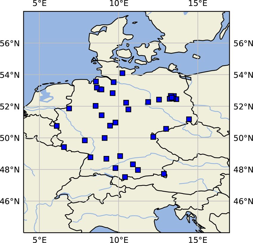
obtained with the graphics PlotStationMap and observation can be viewed in the PlotTimeSeries (not
PlotAvailability. PlotStationMap (Fig. 6) included as a figure in this article). However, since this plot
marks the geographical position of the stations used on a has to scale according to the length of the time series, it
plain map with a land–sea mask, country boundaries, and should be noted that this last-mentioned graph is kept very
major water bodies. The data availability chart created by simple and is generally not suitable for publication.
PlotAvailability (Fig. 7) indicates the time periods
for which preprocessed data for each measuring station 3.3 Statistical analysis of results
are available. The lowest bar shows whether a station with
measurements is available at all for a certain point in time. A central element of MLAir is the statistical evaluation of
The three subsets of training, validation, and testing data are the results according to state-of-the-art methods used in me-
highlighted in different colours. teorology. To obtain specific information on the forecasting
The monitoring graphics show the course of the loss func- model, we treat forecasts and observations as random vari-
tion as well as the error depending on the epoch for the train- ables. Therefore, the joint distribution p(m, o) of a model
ing and validation data (see Fig. 8). In addition, the error of m and an observation o contains information on p(m), p(o)
the best model state with respect to the validation data is (marginal distribution), and the relations p(o|m) and p(m|o)
shown in the plot title. If the learning rate is modified dur- (conditional distribution) between both of them (Murphy and
ing the course of the experiment, another plot is created to Winkler, 1987). Following Murphy et al. (1989), marginal
show its development. These monitoring graphics are kept distribution is shown as a histogram (light grey), while the
as simple as possible and are meant to provide insight into conditional distribution is shown as percentiles in differ-
the training process. The underlying data are always stored ent line styles. By using PlotConditionalQuantiles,
in the JavaScript Object Notation format (.json, ISO Central MLAir automatically creates plots for the entire test period
Secretary, 2017) in the subfolder model and can therefore (Fig. 10) that are, as is common in meteorology, separated
be used for case-specific analyses and plots. by seasons.
Through the graphs PlotMonthlySummary and In order to access the genuine added value of a new fore-
PlotTimeSeries it is possible to quickly as- casting model, it is essential to take other existing forecasting
sess the forecast quality of the ML model. The models into account instead of reporting only metrics related
PlotMonthlySummary (see Fig. 9) summarizes all to the observation. In MLAir we implemented three types of
basic reference forecasts: (i) a persistence forecast, (ii) an or-
Geosci. Model Dev., 14, 1553–1574, 2021 https://doi.org/10.5194/gmd-14-1553-2021L. H. Leufen et al.: MLAir (v1.0) 1561
Figure 6. Map of central Europe showing the locations of
some sample measurement stations as blue squares created by
PlotStationMap.
dinary multi-linear least square model, and (iii) four climato-
logical forecasts.
The persistence forecast is based on the last observed time
step, which is then used as a prediction for all lead times.
The ordinary multi-linear least square model serves as a lin-
ear competitor and is derived from the same data the model
was trained with. For the climatological references, we fol-
low Murphy (1988) who defined single and multiple valued
climatological references based on different timescales. We
refer the reader to Murphy (1988) for an in-depth discussion
of the climatological reference. Note that this kind of persis-
tence and also the climatological forecast might not be appli-
cable for all temporal resolutions and may therefore need ad-
justment in different experiment settings. We think here, for
example, of a clear diurnal pattern in temperature, for which
a persistence of successive observations would not provide a
good forecast. In this context, a reference forecast based on
the observation of the previous day at the same time might
be more suitable.
For the comparison, we use a skill score S, which is natu-
rally defined as the performance of a new forecast compared
to a competitive reference with respect to a statistical metric
(Murphy and Daan, 1985). Applying the mean squared error
Figure 5. Default structure of each MLAir experiment with the sub- as the statistical metric, such a skill score S reduces to unity
folders forecasts, latex_report, logging, model, and minus the ratio of the error of the forecast to the reference.
plots. is a placeholder for the actual name of the A positive skill score can be interpreted as the percentage of
experiment. improvement of the new model forecast in comparison to the
reference. On the other hand, a negative skill score denotes
that the forecast of interest is less accurate than the referenc-
https://doi.org/10.5194/gmd-14-1553-2021 Geosci. Model Dev., 14, 1553–1574, 20211562 L. H. Leufen et al.: MLAir (v1.0)
Figure 7. PlotAvailability diagram showing the available data for five measurement stations. The different colours denote which
period of the time series is used for the training (orange), validation (green), and test (blue) data set. “Data availability” denotes if any of the
above-mentioned stations has a data record for a given time.
Figure 8. Monitoring plots showing the evolution of train and vali- Figure 9. Graph of PlotMonthlySummary showing the obser-
dation loss as a function of the number of epochs. This plot type is vations (green) and the predictions for all forecast steps (dark to
kept very simplistic by choice. The underlying data are saved during light blue) separated for each month.
the experiment so that it would be easy to create a more advanced
plot using the same data.
ensures that the model is provided only with values from
a known range and does not extrapolate out-of-sample. Af-
ing forecast. Consequently, a value of zero denotes that both terwards, the skill scores of the bootstrapped predictions are
forecasts perform equally (Murphy, 1988). calculated using the original forecast as reference. Input vari-
The PlotCompetitiveSkillScore (Fig. 11) in- ables that show an overly negative skill score during boot-
cludes the comparison between the trained model, the persis- strapping have a stronger influence on the prediction than in-
tence, and the ordinary multi-linear least squared regression. put variables with a small negative skill score. In case the
The climatological skill scores are calculated separately for bootstrapped skill score even reaches the positive value do-
each forecast step (lead time) and summarized as a box-and- main, this could be an indication that the examined vari-
whiskers plot over all stations and forecasts (Fig. 12), and as able has no influence on the prediction at all. The result
a simplified version showing the skill score only (not shown) of this approach applied to all input variables is presented
using PlotClimatologicalSkillScore. in PlotBootstrapSkillScore (Fig. 13). A more de-
In addition to the statistical model evaluation, MLAir also tailed description of this approach is given in Kleinert et al.
allows the importance of individual input variables to be as- (2021).
sessed through bootstrapping of individual input variables.
For this, the time series of each individual input variable is
resampled n times (with replacement) and then fed to the
trained network. By resampling a single input variable, its
temporal information is disturbed, but the general frequency
distribution is preserved. The latter is important because it
Geosci. Model Dev., 14, 1553–1574, 2021 https://doi.org/10.5194/gmd-14-1553-2021L. H. Leufen et al.: MLAir (v1.0) 1563
fied and the authors’ choices for default settings when using
the default workflow of MLAir.
4.1 Host system and processing units
The MLAir workflow can be adjusted to the hosting sys-
tem. For that, the local paths for experiment and data are
adjustable (see Table 1 for all options). Both paths are sep-
arated by choice. This has the advantage that the same data
can be used multiple times for different experiment setups
if stored outside the experiment path. Contrary to the data
path placement, all created plots and forecasts are saved in
the experiment_path by default, but this can be adjusted
through the plot_path and forecast_path parameter.
Concerning the processing units, MLAir supports both
Figure 10. Conditional quantiles in terms of calibration-refinement central processing units (CPUs) and GPUs. Due to their
factorization for the first lead time and the full test period. The bandwidth optimization and efficiency on matrix opera-
marginal forecasting distribution is shown as a log histogram in tions, GPUs have become popular for ML applications (see
light grey (counting on right axis). The conditional distribution (cal- Krizhevsky et al., 2012). Currently, the sample models im-
ibration) is shown as percentiles in different line styles. Calcula- plemented in MLAir are based on TensorFlow v1.13.1, which
tions are done with a bin size of 1 ppb. Moreover, the percentiles has distinct branches: the tensorflow-1.13.1 package for CPU
are smoothed by a rolling mean of window size three. This kind of computation and the tensorflow-gpu-1.13.1 package for GPU
plot was originally proposed by Murphy et al. (1989) and can be
devices. Depending on the operating system, the user needs
created using PlotConditionalQuantiles.
to install the appropriate library if using TensorFlow releases
1.15 and older (TensorFlow, 2020). Apart from this installa-
tion issue, MLAir is able to detect and handle both Tensor-
Flow versions during run time. An MLAir version to support
TensorFlow v2 is planned for the future (see Sect. 5).
4.2 Preprocessing
In the course of preprocessing, the data are prepared to al-
low immediate use in training and evaluation without further
preparation. In addition to the general data acquisition and
formatting, which will be discussed in Sect. 4.3 and 4.4, pre-
processing also handles the split into training, validation, and
test data. All parameters discussed in this section are listed in
Table 2.
Data are split into subsets along the temporal axis
and station between a hold-out data set (called test
Figure 11. Skill scores of different reference models like data) and the data that are used for training (train-
persistence (persi) and ordinary multi-linear least square ing data) and model tuning (validation data). For
(ols). Skill scores are shown separately for all forecast steps each subset, a {train,val,test}_start and
(dark to light blue). This graph is generated by invoking {train,val,test}_end date not exceeding the overall
PlotCompetitiveSkillScore. time span (see Sect. 4.4) can be set. Additionally, for
each subset it is possible to define a minimal number of
samples per station {train,val,test}_min_length
4 Configuration of experiment, data handler, and to remove very short time series that potentially cause
model class in the MLAir workflow misleading results especially in the validation and test phase.
A spatial split of the data is achieved by assigning each
As well as the already described workflow adjustments, station to one of the three subsets of data. The parameter
MLAir offers a large number of configuration options. In- fraction_of_training determines the ratio between
stead of defining parameters at different locations inside the hold-out data and data for training and validation, where
code, all parameters are centrally set in the experiment setup. the latter two are always split with a ratio of 80 % to 20 %,
In this section, we describe all parameters that can be modi- which is a typical choice for these subsets.
https://doi.org/10.5194/gmd-14-1553-2021 Geosci. Model Dev., 14, 1553–1574, 20211564 L. H. Leufen et al.: MLAir (v1.0)
Figure 12. Climatological skill scores (cases I to IV) and related terms of the decomposition as proposed in Murphy (1988) created by
PlotClimatologicalSkillScore. Skill scores and terms are shown separately for all forecast steps (dark to light blue). In brief,
cases I to IV describe a comparison with climatological reference values evaluated on the test data. Case I is the comparison of the forecast
with a single mean value formed on the training and validation data and case II with the (multi-value) monthly mean. The climatological
references for cases III and IV are, analogous to cases I and II, the single and the multi-value mean, but on the test data. Cases I to IV are
calculated from the terms AI to CIV. For more detailed explanations of the cases, we refer to Murphy (1988).
Table 1. Summary of all parameters related to the host system that are required, recommended, or optional to adjust for a custom experiment
workflow.
Host system
Parameter Default Adjustment
experiment_date testrun recommended
experiment_name {experiment_date}_network –a
experiment_path hcwdb i/{experiment_name} optional
data_path hcwdb i/data optional
bootstrap_path hdata_pathi/bootstraps optional
forecast_path hexperiment_pathi/forecasts optional
plot_path hexperiment_pathi/plots optional
a Only adjustable via the experiment_date parameter.
b Refers to the Linux command to get the path name of the current working directory.
To achieve absolute statistical data subset independence, vision, the amount of utilizable data can drop massively. In
data should ideally be split along both temporal and spatial MLAir, it is therefore up to the user to split data either in the
dimensions. Since the spatial dependency of two distinct sta- temporal dimension or along both dimensions by using the
tions may vary due to weather regimes, season, and time of use_all_stations_on_all_data_sets parameter.
day (Wilks, 2011), a spatial and temporal division of the data
might be useful, as otherwise a trained model can presum-
ably lead to over-confident results. On the other hand, by
applying a spatial split in combination with a temporal di-
Geosci. Model Dev., 14, 1553–1574, 2021 https://doi.org/10.5194/gmd-14-1553-2021L. H. Leufen et al.: MLAir (v1.0) 1565
Figure 13. Skill score of bootstrapped model input predictions separated for each input variable (x axis) and forecast steps (dark to light
blue) with the original (non-bootstrapped) predictions as reference. PlotBootstrapSkillScore is only executed if bootstrap analysis
is enabled.
Table 2. Summary of all parameters related to the preprocessing that are required, recommended, or optional to adjust for a custom experiment
workflow.
Preprocessing
Parameter Default Adjustment
stations default stationsa recommended
data_handler DefaultDataHandler optional
fraction_of_training 0.8 optionalb
use_all_stations_on_all_data_sets True optional
a Default stations: DEBW107, DEBY081, DEBW013, DEBW076, DEBW087.
b Not used in the default setup because use_all_stations_on_all_data_sets is True.
4.3 Custom data handler origin, while the iteration and distribution into batches is
taken care of while MLAir is running.
The integration of a custom data handler into the The accessor methods for input and target data form a
MLAir workflow is done by inheritance from the clearly defined interface between MLAir’s run modules and
AbstractDataHandler class and implementation the custom data handler. During training the data are needed
of at least the constructor __init__(), and the accessors as a NumPy array; for preprocessing and evaluation the data
get_X(), and get_Y(). The custom data handler is are partly used as xarray. Therefore the accessor methods
added to the MLAir workflow as a parameter without ini- have the parameter as_numpy and should be able to return
tialization. At runtime, MLAir then queries all the required both formats. Furthermore it is possible to use a custom up-
parameters of this custom data handler from its arguments sampling technique for training. To activate this feature the
and keyword arguments, loads them from the data store and parameter upsampling can be enabled. If such a technique
finally calls the constructor. If data need to be downloaded or is not used and therefore not implemented, the parameter has
preprocessed, this should be executed inside the constructor. no further effect.
It is sufficient to load the data in the accessor methods if The abstract data handler provides two additional place-
the data can be used without conversion. Note that a data holder methods that can support data preparation, training,
handler is only responsible for preparing data from a single and validation. Depending on the case, it may be helpful to
https://doi.org/10.5194/gmd-14-1553-2021 Geosci. Model Dev., 14, 1553–1574, 20211566 L. H. Leufen et al.: MLAir (v1.0)
Table 3. Summary of all parameters related to the default data han- ID. By default, the DefaultDataHandler uses all Ger-
dler that are required, recommended, or optional to adjust for a cus- man air quality stations provided by the German Environ-
tom experiment workflow. ment Agency (Umweltbundesamt, UBA) that are indicated
as “background” stations according to the European Envi-
Default data handler ronmental Agency (EEA) AirBase classification (European
Parameter Default Adjustment Parliament and Council of the European Union, 2008). Using
data_path see Table 1 optional
the stations parameter, a user-defined data collection can
stations default stationsa recommended be created. To filter the stations, the parameters network
network – optional and station_type can be used as described in Schultz
station_type – optional et al. (2017a) and the documentation of JOIN (Schultz and
variables default variablesb recommended Schröder, 2017).
statistics_per_var default statisticsb recommended For the DefaultDataHandler, it is recommended to
target_var o3 recommended
specify at least
start 1997-01-01 recommended
end 2017-12-31 recommended – the number of preceding time steps to use for a single
sampling daily optional
window_history_size 13 recommended
input sample (window_history_size),
interpolation_method linear optional
limit_nan_fill 1 optional
– if and which interpolation should be used
min_lengthc 0 optional (interpolation_method),
window_lead_time 3 recommended
overwrite_local_data False optional – if and how many missing values are allowed to be filled
by interpolation (limit_nan_fill),
a Default stations: DEBW107, DEBY081, DEBW013, DEBW076, DEBW087.
b Default variables (statistics): o3 (dma8eu), relhum (average_values), temp (maximum), u
(average_values), v (average_values), no (dma8eu), no2 (dma8eu), cloudcover
– and how many time steps the forecast model should pre-
(average_values), pblheight (maximum). dict (window_lead_time).
c Indicates the required minimum number of samples per station.
Regarding the data content itself, each requested variable
must be added to the variables list and be part of the
define these methods within a custom data handler. With the statistics_per_var dictionary together with a proper
method transformation it is possible to either define or statistic abbreviation (see documentation of Schultz and
calculate the transformation properties of the data handler be- Schröder, 2017). If not provided, both parameters are cho-
fore initialization. The returned properties are then applied to sen from a standard set of variables and statistics. Similar
all subdata sets, namely training, validation, and testing. An- actions are required for the target variable. Firstly, target vari-
other supporting class method is get_coordinates. This ables are defined in target_var, and secondly, the target
method is currently used only for the map plot for geograph- variable must also be part of the statistics_per_var
ical overview (see Sect. 3.2). To feed the overview map, this parameter. Note that the JOIN REST API calculates these
method must return a dictionary with the geographical coor- statistics online from hourly values, thereby taking into ac-
dinates indicated by the keys lat and lon. count a minimum data coverage criterion. Finally, the over-
all time span the data shall cover can be defined via start
4.4 Default data handler and end, and the temporal resolution of the data is set by
a string like "daily" passed to the sampling parameter.
In this section we describe a concrete implementation of a At this point, we want to refer to Sect. 5, where we discuss
data handler, namely the DefaultDataHandler, using the temporal resolution currently available.
data from the JOIN interface.
Regarding the data handling and preprocessing, several pa- 4.5 Defining a model class
rameters can be set to control the choice of inputs, size of
data, etc. in the data handler (see Table 3). First, the under- The motivation behind using model classes was already ex-
lying raw data must be downloaded from the web. The cur- plained in Sect. 2.4. Here, we show more details on the im-
rent version of the DefaultDataHandler is configured plementation and customization.
for use with the REST API of the JOIN interface (Schultz To achieve the goal of an easy plug-and-play behaviour,
and Schröder, 2017). Alternatively, data could be already each ML model implemented in MLAir must inherit from the
available on the local machine in the directory data_path, AbstractModelClass, and the methods set_model
e.g. from a previous experiment run. Additionally, a user and set_compile_options are required to be over-
can force MLAir to load fresh data from the web by en- written for the custom model. Inside set_model, the
abling the overwrite_local_data parameter. Accord- entire model from inputs to outputs is created. Thereby
ing to the design structure of a data handler, data are han- it has to be ensured that the model is compatible with
dled separately for each observational station indicated by its Keras to be compiled. MLAir supports both the functional
Geosci. Model Dev., 14, 1553–1574, 2021 https://doi.org/10.5194/gmd-14-1553-2021L. H. Leufen et al.: MLAir (v1.0) 1567
and sequential Keras application programming interfaces. the model used itself must be provided to MLAir including
For details on how to create a model with Keras, we additional hyperparameters like the learning_rate, the
refer to the official Keras documentation (Chollet et al., algorithm to train the model (optimizer), and the loss
2015). All options for the model compilation should be function to measure model performance. For more details
set in the set_compile_options method. This method on how to implement an ML model properly we refer to
should at least include information on the training al- Sect. 4.5.
gorithm (optimizer), and the loss to measure perfor- Due to its application focus on meteorological time series
mance during training and optimize the model for (loss). and therefore on solving a regression problem, MLAir offers
Users can add other compile options like the learning rate a particular handling of training data. A popular technique
(learning_rate), metrics to report additional in- in ML, especially in the image recognition field, is to aug-
formative performance metrics, or options regarding the ment and randomly shuffle data to produce a larger number
weighting as loss_weights, sample_weight_mode, of input samples with a broader variety. This method requires
or weighted_metrics. Finally, methods that are not part independent and identically distributed data. For meteoro-
of Keras or TensorFlow like customized loss functions or logical applications, these techniques cannot be applied out
self-made model extensions are required to be added as so- of the box, because of the lack of statistical independence
called custom_objects to the model so that Keras can of most data and autocorrelation (see also Schultz et al.,
properly use these custom objects. For that, it is necessary to 2021). To avoid generating over-confident forecasts, training
call the set_custom_objects method with all custom and test data are split into blocks so that little or no over-
objects as key value pairs. See also the official Keras docu- lap remains between the data sets. Another common problem
mentation for further information on custom objects. in ML, not only in the meteorological context, is the natu-
An example implementation of a small model using a sin- ral under-representation of extreme values, i.e. an imbalance
gle convolution and three fully connected layers is shown in problem. To address this issue, MLAir allows more empha-
Fig. 14. By inheriting from the AbstractModelClass sis to be placed on such data points. The weighting of data
(l. 9), invoking its constructor (l. 15), defining the methods samples is conducted by an over-representation of values that
set_model (l. 25–35) and set_compile_options can be considered as extreme regarding the deviation from a
(l. 37–41), and calling these two methods (l. 21–22), the cus- mean state in the output space. This can be applied during
tom model is immediately usable for MLAir. Additionally, training by using the extreme_values parameter, which
the loss is added to the custom objects (l. 23). This last step defines a threshold value at which a value is considered ex-
would not be necessary in this case, because an error func- treme. Training samples with target values that exceed this
tion incorporated in Keras is used (l. 2/40). For the purpose limit are then used a second time in each epoch. It is also pos-
of demonstrating how to use a customized loss, it is added sible to enter more than one value for the parameter. In this
nevertheless. case, samples with values that exceed several limits are du-
A more elaborate example is described in Kleinert et al. plicated according to the number of limits exceeded. For pos-
(2021), who used extensions to the standard Keras library in itively skewed distributions, it could be helpful to apply this
their workflow. So-called inception blocks (Szegedy et al., over-representation only on the right tail of the distribution
2015) and a modification of the two-dimensional padding (extremes_on_right_tail_only). Furthermore, it is
layers were implemented as Keras layers and could be used possible to shuffle data within, and only within, the training
in the model afterwards. subset randomly by enabling permute_data.
4.6 Training 4.7 Validation
The parameter create_new_model instructs MLAir to The configuration of the ML model validation is related to
create a new model and use it in the training. This is nec- the postprocessing stage. As mentioned in Sect. 2.3, in the
essary, for example, for the very first training run in a new default configuration there are three major validation steps
experiment. However, it must be noted that already existing undertaken after each run besides the creation of graph-
training progress within the experiment will be overwritten ics: first, the trained model is opposed to the two reference
by activating create_new_model. Independent of using models, a simple linear regression and a persistence predic-
a new or already existing model, train_model can be tion. Second, these models are compared with climatological
used to set whether the model is to be trained or not. Fur- statistics. Lastly, the influence of each input variable is esti-
ther notes on the continuation of an already started training mated by a bootstrap procedure.
or the use of a pre-trained model can be found in Sect. 4.9. Due to the computational burden the calculation of the in-
Most parameters to set for the training stage are re- put variable sensitivity can be skipped and the graphics cre-
lated to hyperparameter tuning (see Table 4). Firstly, the ation part can be shortened. To perform the sensitivity study,
batch_size can be set. Furthermore, the number of the parameter evaluate_bootstraps must be enabled
epochs to train needs to be adjusted. Last but not least, and the number_of_bootstraps defines how many
https://doi.org/10.5194/gmd-14-1553-2021 Geosci. Model Dev., 14, 1553–1574, 2021You can also read


