Using a multi-hypothesis framework to improve the understanding of flow dynamics during flash floods - HESS
←
→
Page content transcription
If your browser does not render page correctly, please read the page content below
Hydrol. Earth Syst. Sci., 22, 5317–5340, 2018
https://doi.org/10.5194/hess-22-5317-2018
© Author(s) 2018. This work is distributed under
the Creative Commons Attribution 4.0 License.

Using a multi-hypothesis framework to improve the understanding
of flow dynamics during flash floods
Audrey Douinot1 , Hélène Roux1 , Pierre-André Garambois2 , and Denis Dartus1
1 Institut   de Mécanique des Fluides de Toulouse (IMFT), University of Toulouse, CNRS – Toulouse, France
2 Laboratoire    des Sciences de l’ingénieur, de l’informatique et de l’imagerie (ICUBE) – INSA Strasbourg, Strasbourg, France

Correspondence: Audrey Douinot (audreydouinot@gmail.com)

Received: 4 December 2017 – Discussion started: 8 December 2017
Revised: 14 September 2018 – Accepted: 18 September 2018 – Published: 16 October 2018

Abstract. A method of multiple working hypotheses was               localised and major forcings (greater than 100 mm; Gaume
applied to a range of catchments in the Mediterranean area          et al., 2009) at the heads of steep-sided, mesoscale catch-
to analyse different types of possible flow dynamics in             ments (with surface areas of 10–250 km2 ).
soils during flash flood events. The distributed, process-             The large specific discharges and intensities of precipita-
oriented model, MARINE, was used to test several repre-             tion lead to the flash floods being classified as extreme. Nev-
sentations of subsurface flows, including flows at depth in         ertheless, those events are not scarce nor unusual, since on
fractured bedrock and flows through preferential pathways           average, there were no fewer than five flash floods a year in
in macropores. Results showed the contrasting performances          the Mediterranean Arc between 1958 and 1994 (Jacq, 1994),
of the submitted models, revealing different hydrological be-       and they tend to be amplified against a background of climate
haviours among the catchment set. The benchmark study of-           change (Llasat et al., 2014; Colmet Daage et al., 2016). Flash
fered a characterisation of the catchments’ reactivity through      floods constitute a significant hazard and are therefore a con-
the description of the hydrograph formation. The quantifi-          siderable risk for populations (UNISDR, 2009; Llasat et al.,
cation of the different flow processes (surface and intra-soil      2014). They are particularly dangerous due to their charac-
flows) was consistent with the scarce in situ observations,         teristics, namely that (i) the suddenness of events makes it
but it remains uncertain as a result of an equifinality issue.      difficult to warn populations in time, and this can lead to
The spatial description of the simulated flows over the catch-      panic, thus increasing the risk when a population is unpre-
ments, made available by the model, enabled the identifica-         pared (Ruin et al., 2008), (ii) the traditional connected mon-
tion of counterbalancing effects between internal flow pro-         itoring systems are not adapted to the temporal and spatial
cesses, including the compensation for the water transit time       scales of the flash floods (Borga et al., 2008; Braud et al.,
in the hillslopes and in the drainage network. New insights         2014), and (iii) the magnitude of floods implies significant
are finally proposed in the form of setting up strategic moni-      amounts of kinetic energy, which can transform transitory
toring and calibration constraints.                                 rivers into torrents, resulting in the transport of debris rang-
                                                                    ing from fine sediments to tree trunks as well as the scouring
                                                                    of river beds and the erosion of banks (Borga et al., 2014).
                                                                       A major area of interest for flash floods is, therefore, better
1     Introduction                                                  risk assessment, which enables them to be forecasted and the
                                                                    relevant populations to be pre-warned. Greater knowledge
1.1    Flash flood events: an issue for forecasters                 and understanding is required to better identify the determin-
                                                                    ing factors that result in flash floods. In particular, in order
Flash floods are “sudden floods with high peak discharges,          to implement a regional forecasting system, the properties of
produced by severe thunderstorms that are generally of lim-         the catchments and the climatic forcing and linkages between
ited areal extent” (IAHS-UNESCO-WMO, 1974; Garam-                   them that lead to flash flood events need to be characterised.
bois, 2012; Braud et al., 2014). They are often linked to

Published by Copernicus Publications on behalf of the European Geosciences Union.
5318       A. Douinot et al.: Using a multi-hypothesis framework to improve the understanding of flash flood dynamics

1.2    Flash flood events: understanding flow processes            the floods mainly consisted of new water, with a proportion
                                                                   varying between 50 % and 80 %, it appears that over the en-
Due to the challenges involved in forecasting flash floods,        tire period of the events, old water accounts for between 70 %
there has been considerable research done on the subject           and 80 % of the total volume of water discharged, which sup-
over the last 10 years. Examples include the HYDRATE (Hy-          ports the dominance of the water pathways in the soil.
drometeorological data resources and technologies for effec-          Finally the geological properties themselves appear to
tive flash flood forecasting, 2006–2010; Gaume and Borga,          be markers of the storage capacities available over the
2013), which enabled the setting up of a comprehensive Eu-         timescales involved in flash floods (that are of the order
ropean database of flash flood flash events as well as the de-     of a day). From simple flow balances of flash flood events
velopment of a reference methodology for the observation of        (Douinot, 2016), studies of the diverse hydrological re-
post-flood events, the EXTRAFLO (EXTreme RAinfall and              sponses of several catchments over the same precipitation
FLOod estimation, 2009–2013; Lang et al., 2014) to estimate        episode (Payrastre et al., 2012) or the application of re-
extreme precipitation and floods for French catchments, the        gional hydrological models dedicated to flash flood sim-
HYMEX project (HYdrological cycle in the Mediterranean             ulation (Garambois et al., 2015b), the literature tends to
EXperiment, 2010–2020; Drobinski et al., 2014) focusing            demonstrate the low storage capacity of non-karst sedimen-
on the meteorological cycle at the Mediterranean scale and         tary catchments and marl-type catchments, and, conversely,
particularly on the conditions that allow extreme events to        the potential for storing large volumes of water in the altered
develop, the FLASH project (Flooded Locations and Simu-            rocks of granitic or schist formations.
lated Hydrographs, 2012–2017; Gourley et al., 2017) assess-
ing the ability and the improvement of a flash flood forecast-     1.3   Applying a multi-hypothesis framework for
ing framework in USA on the basis of real-time hydrologi-                improving the hydrological understanding of the
cal modelling with high-resolution forcing, or the FLOOD-                flash flood events
SCALE project (Multi-scale hydrometeorological observa-
tion and modelling for flash floods understanding and sim-         The knowledge gained about the development of the flow
ulation, 2012–2016; Braud et al., 2014), based on a multi-         processes (for example, the tracing of events carried out dur-
scale experimental approach to improve the observation of          ing the FLOODSCALE project; Braud et al., 2014) relates to
the hydrological processes that lead to flash floods.              studies on a number of specific sites where flash floods could
   In the northwestern Mediterranean context – especially          be observed while they were taking place. However, being
concerned with specific autumnal convective meteorologi-           able to generalise the knowledge gained is limited by the spe-
cal events – the European cited research particularly demon-       cific nature of each study (McDonnell et al., 2007) and by the
strates the importance of cumulative rainfall (Arnaud et al.,      gap between the spatial scale of forecasts (mesoscale) com-
1999; Sangati et al., 2009; Camarasa-Belmonte, 2016), the          pared with that of the in situ observations (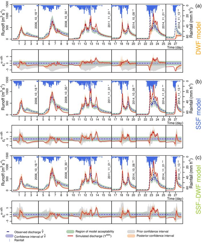
A. Douinot et al.: Using a multi-hypothesis framework to improve the understanding of flash flood dynamics                  5319

                                                                   2011; Garambois et al., 2015a), which was developed specif-
                                                                   ically to model flash floods in the catchments of the French
                                                                   Mediterranean Arc. Several new representations for the soil
                                                                   column and underground flows were proposed (Douinot,
                                                                   2016) and included in the MARINE model in the form of
                                                                   modules that can be used to test different hydrological func-
                                                                   tions (Sect. 3). Those different hydrological dynamics were
                                                                   applied to a set of catchments, presented in Sect. 2, with
                                                                   physiographic properties representative of the whole of the
                                                                   French Mediterranean Arc. The performance of each model
                                                                   was then examined and subjected to a comparative study
                                                                   (Sects. 4 and 5). The contributions of the results for improv-
                                                                   ing the hydrological functioning understanding are lastly dis-
                                                                   cussed in Sect. 6 before concluding.

Figure 1. Locations of the catchments studied, with a topo-
graphic visualisation at a resolution of 25 m (Source – IGN; MNT   2     Catchments and data used in the study
BDALTI).
                                                                   2.1    Study catchment set
work, such as FUSE (Framework for Understanding Struc-             We studied the behaviour of four catchments and eight nested
tural Errors, Clark et al., 2008) or SUPERFLEX (Flexible           catchments in the French Mediterranean Arc (Fig. 1). The
framework for hydrological modeling, Fenicia et al., 2011).        catchments (in the order they are numbered in Fig. 1) were
However, Clark et al. (2015a, b) have also proposed a uni-         those of the Ardèche, Gard, Hérault and Salz rivers. These
fied structure to test multiple working hypotheses within a        were selected for the following reasons; (i) they are represen-
distributed modeling framework. To our knowledge, the case         tative of the physiographic variability found in areas where
studies using the aforementioned frameworks are related to         flash floods occur, (ii) numerous studies of flash floods have
continuous hydrological studies in order to assess hydrolog-       already been carried out on the Gard and Ardèche (Ruin
ical hypotheses through the overall hydrological signature of      et al., 2008; Anquetin et al., 2010; Delrieu et al., 2005;
the catchments. In this work, we extend the method of multi-       Maréchal et al., 2009; Braud et al., 2014) that could guide the
ple working hypotheses to the assessment of an event-based         interpretation of the modelling results (Fenicia et al., 2014),
hydrological model framework.                                      and (iii) a considerable number of observations of flash flood
   The objective is to test a number of proposed hydrologi-        events are available for these catchments.
cal mechanisms that occur during flash flood events in a set          The main physiographical and hydrological properties of
of contrasting catchments in the French Mediterranean area.        the catchments are presented in Table 1. Figure 2 shows
While the proportion of flows passing through the soil ap-         the contrasting geological properties of the studied area; the
pears to be significant, questions arise about how they form:      catchments are marked by a clear upstream–downstream dif-
                                                                   ference. The Ardèche catchment upstream of Ucel essentially
  – Are they subsurface flows that take place in a restricted
                                                                   sits on a granite bedrock with some sandstone on its edges,
    area of the root layer as a result of preferential path ac-
                                                                   while downstream the geology changes to predominantly
    tivation? Or are they lateral flows taking place at greater
                                                                   schist and limestone formations. Similarly, the upstream part
    depth, comparable to those seen in some aquifers?
                                                                   of the Gard catchment consists of schistose bedrock, while
  – Does the geological bedrock or an altered substratum           downstream the bedrock is impermeable marl-type and gran-
    play a role limited to that of mere storage reservoir, or      ite formations. The Hérault catchment is split into mostly
    is it actively involved in flood flows formation?              schist and granitic head watersheds (the Valleraugue and
                                                                   la Terrisse sub-catchments) and is a predominantly lime-
  – Which are the flow processes proportions, according to         stone plateau (Saint-Laurent-le-Minier sub-catchment). Fi-
    the events and the catchments?                                 nally, the Salz is characterised by sedimentary bedrock com-
                                                                   prised of sandstone and limestone (Fig. 2).
   The aim of this article is to attempt to answer these ques-        The Ardèche and the Gard catchments have been subject to
tions using a multi-model approach that tests different types      intensive monitoring and studies (see later references, https:
of hydrological dynamics. The study was based on MA-               //deims.org/site/czo_eu_fr_024, last access: 10 May 2018),
RINE (Modélisation de l’Anticipation du Ruissellement et           leading to prior knowledge on hydrological understanding.
des Inondations pour des évéNements Extrêmes), a phys-             Both the local in situ experiments (Ribolzi et al., 1997; Braud
ically based, distributed hydrological model (Roux et al.,         and Vandervaere, 2015; Braud et al., 2016a, b) and the mod-

www.hydrol-earth-syst-sci.net/22/5317/2018/                                      Hydrol. Earth Syst. Sci., 22, 5317–5340, 2018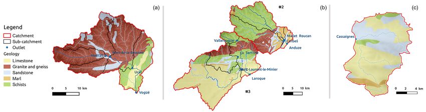
A. Douinot et al.: Using a multi-hypothesis framework to improve the understanding of flash flood dynamics

                                                                                                                                                                                                                                                                                                         www.hydrol-earth-syst-sci.net/22/5317/2018/
                                                                                                             Table 1. Physiographic properties and hydrological statistics of the 12 catchments. Here, ID is the coding name of the catchments used at Fig. 1 and Table 2, and the following are
                                                                                                             represented: area (km2 ), mean slope (–), soil properties of mean soil depth (m) and main soil texture (Tx), sandy loam texture = (Ls), loam texture = (L), silty loam texture = (Lsi).
                                                                                                             In terms of geology, the following are represented: percentage of bedrock geology (%), including subcategories of sandstone (Sa), limestone (Li), granite and gneiss (GG), marl (Ma)
                                                                                                             and schists (Sc). (i) Bold values represent the dominant geology. Mean annual precipitation is P (mm). In terms of hydrometry, period is the discharge time-series availability, the mean
                                                                                                             inter-annual discharge is Q (m3 km−2 s−1 ), the 2 year return period of maximum daily discharge is QD2 (m3 km−2 s−1 ), and the 10 year return period of maximum hourly discharge
                                                                                                             is QH10 (m3 km−2 s−1 ). Hydrometric statistics are calculated from HydroFrance databank (http://www.hydro.eaufrance.fr/, last access: 10 May 2018), and the pluviometric ones using
                                                                                                             rainfall data are from the rain gauge network of the French flood forecasting services.
                                                                                                              ID        River         Outlet                                        Soil properties                   Geology(i)                                  Hydrometry
                                                                                                                                                                   Area    Slope    Depth     Tx        Sa      Li       GG        Ma      Sc      P        Q QD2 QH10             Period
                                                                                                                                                                  (km2 )     (−)      (m)     (−)      (%)     (%)       (%)       (%)    (%)    (mm)       (m3 km−2 s−1 )         Period
                                                                                                              no. 1a    L’Ardèche     Vogüé                         622     0.17      0.47    Ls       10.5     5.7     71.9       0.0    11.9   1587   0.041    0.62      2.25    00–15
                                                                                                              no. 1b                  Ucel                          477     0.20      0.45    Ls       13.7     0.0     84.5       0.0     1.8   1577   0.046    0.79      2.30    05–15
                                                                                                              no. 1c                  Pont-de-la-Beaume             292     0.22      0.39    Ls       14.0     0.0     86.0       0.0     0.0   1690   0.056    0.75      2.53    00–15
                                                                                                              no. 1d                  Meyras                         99     0.24      0.32    Ls        5.4     0.0     94.6       0.0     0.0   1720   0.036    0.72      2.92    00–15
                                                                                                              no. 2a    Le Gardon     Anduze                        543     0.16      0.25    L         7.2     1.5     18.0   12.1       61.2   1370   0.026    0.48      1.82    94–15
                                                                                                              no. 2b                  Corbès                        220     0.16      0.27    L         9.3     0.0     34.2    9.0       47.5   1460   0.022    0.57      2.28    94–15

                                                                                                                                                                                                                                                                                                         Hydrol. Earth Syst. Sci., 22, 5317–5340, 2018
                                                                                                              no. 2c                  Mialet Roucan                 240     0.17      0.22    L         2.0     0.6      2.9    9.4       85.1   1407   0.023    0.62      2.54    02–15
                                                                                                              no. 3a    L’Hérault     Laroque                       912     0.14      0.26    Lsi       6.7   54.5      11.7       3.2    24.0   1160   0.019    0.39      1.21    00–15
                                                                                                              no. 3b    La Vis        Saint-Laurent-le-Minier       499     0.10      0.26    Lsi       4.0   83.0       1.0       3.2     8.8    930   0.018    0.42      1.10    00–15
                                                                                                              no. 3c    L’Arre        La Terrisse                   155     0.19      0.25    L        19.5   12.3      27.2       6.2    34.8   1130   0.027    0.61       2.0    00–15
                                                                                                              no. 3d    L’Hérault     Valleraugue                    46     0.27      0.25    L         0.0    0.0       0.0       0.0   100.0   1920   0.049    1.13       4.0    08–15
                                                                                                              no. 4     La Salz       Cassaigne                     144     0.13      0.37    Lsi      33.5   56.5       0.0       5.1     4.9    700   0.008    0.20      1.31    01–15
5320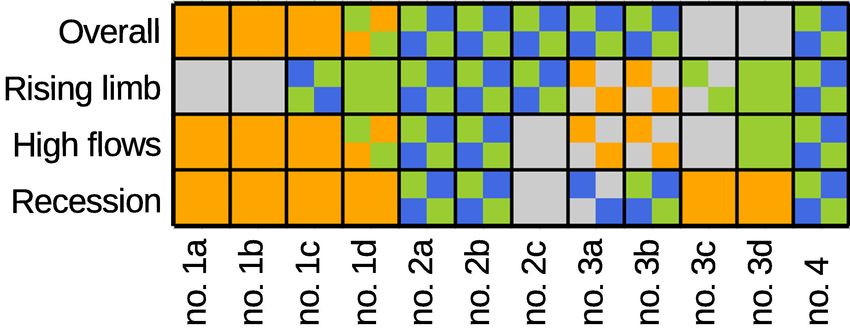
A. Douinot et al.: Using a multi-hypothesis framework to improve the understanding of flash flood dynamics                         5321

Figure 2. The geology of the Ardèche catchment (a), the Gard and Hérault catchments (b), and the Salz catchment (c) (sources: BD Million-
Géol, BRGM).

elling studies focused on this area (Garambois et al., 2013;           ing centres in France) were selected as events to be included
Vannier et al., 2013) tend to support a hydrological classifica-       in the study. Thus, only one criterion for hydrological re-
tion according to those contrasting geological properties, in          sponse was considered. This led to a selection of precipita-
agreement with the usual hydrogeological signature found in            tion events of varying origins (for instance, rainfall induced
the literature (Sayama et al., 2011; Pfister et al., 2017a). Marl,     by mountains, stagnant convective cells and rainfall occur-
sandstone and limestone without karst are characterised by             ring in different seasons, mainly in autumn and early spring).
limited storage capacities, resulting in higher runoff coef-           Such a selection risked complicating the study because flow
ficients and high sensitivity to the initial soil moisture (Ri-        processes can vary from one season to another. Nevertheless,
bolzi et al., 1997; Braud et al., 2016a). In contrast, in granite      it allowed us to test the ability of the model to deal with dif-
and schist transects located on the hillslope of the Ardèche           ferent (non-linear) flow physics regimes. Note also that mod-
catchment, infiltration tests and analyses of electrical resis-        erate or intense rainfall events without respective hydrologi-
tivity signals show the high permeability of the geological            cal responses might be taken out of the analysis. Nevertheless
substratum in depth (measured up to 2.5 m in depth); high              the first alert threshold used here is small enough to have a
storage capacities reach up to 600 mm in 7 out of 10 as-               selection of flood events with contrasting runoff coefficients
sessments with artificial forcing and the three remaining tests        (see Table 2).
suggest local unaltered bedrock (Braud et al., 2016a, b). The             Precipitation measurements were taken from Météo
natural resistivity profile suggests a regular soil bedrock in-        France’s ARAMIS (Application Radar à la Météorolo-
terface when the latter consists of schist, while the granite          gie Infra-Synoptique) radar network (Tabary, 2007), which
one presents a more chaotic structure. Finally, the continuous         provides precipitation measurements at a resolution of
comparative study of two experimental sites over surface ar-           1 km × 1 km every 5 min. The French flood forecasting ser-
eas of the order of 1 km2 – one located on the schist upstream         vice (SCHAPI – Service central d’hydrométéorologie et
part of the Gard catchment and the other one on the down-              d’appui à la prévision des inondations) then used the CALA-
stream granite part – suggests that there is rapid subsurface          MAR patented software (Badoche-Jacquet et al., 1992) to
flow processing on the schist area, while flow formation ap-           produce rainfall depth data by combining these radar mea-
pears to be controlled by the extension of the saturated zone          surements with rain gauge data. This processed dataset is
related to the river on the granitic site (Ayral et al., 2005;         used here as inputs for the model. Each rainfall product is
Maréchal et al., 2009, 2013).                                          firstly assessed through an individual sensitivity analysis of
                                                                       the standard MARINE model (DWF model; see Sect. 3.1).
2.2   Forcing inputs and hydrometric data                              When presenting an atypical sensitivity to the soil depth pa-
                                                                       rameter, the rainfall event is discarded in the study, as it sug-
The hydrometric data were derived from the network of oper-            gests questionable measurements. Depending on the avail-
ational measurements (HydroFrance databank, http://www.                ability of the results of rainfall and hydrometric measure-
hydro.eaufrance.fr/, last access: 10 May 2018). Eight to               ments, 7 to 14 intense events were selected for each catch-
twenty years of hourly discharge observations were avail-              ment (Table 2). Each set is finally split into calibration and
able, according to the dates when the hydrometric stations             validation subsets as follows; the extreme events were kept
were installed (Table 1).                                              for validation, and a minimum of three calibration events are
   Flood events with peak discharges that had exceeded the             chosen in order to cover the wide range of initial soil mois-
2 year return period for daily discharge (QD2 in Table 1,              ture conditions.
which corresponds to the alert threshold for flood forecast-

www.hydrol-earth-syst-sci.net/22/5317/2018/                                          Hydrol. Earth Syst. Sci., 22, 5317–5340, 2018
5322 A. Douinot et al.: Using a multi-hypothesis framework to improve the understanding of flash flood dynamics
E
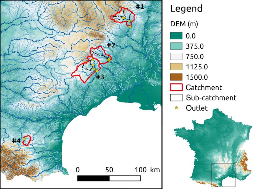
Figure 3. The MARINE model structure, parameters and variables. The Green–Ampt infiltration equation contains the following parameters:
infiltration rate i (m s−1 ), cumulative infiltration I (mm), saturated hydraulic conductivity K (m s−1 ), soil suction at the wetting front 9 (m),
and saturated and initial water contents, θs and θi (m3 m−3 ), respectively. Subsurface flow contains the following parameters: soil thickness
(m), lateral saturated hydraulic conductivity K (m s−1 ), local water depth h (m), transmissivity decay with depth mh (m) and bed slope S
(m m−1 ). The kinematic wave contains the following parameters: surface water depth h (m), time t (s), space variable x (m), rainfall rate r
(m s−1 ), infiltration rate i (m s−1 ), bed slope S (m m−1 ) and Manning roughness coefficient n (m−1/3 s). Module 2 described in this figure
corresponds to the standard definition applied in the MARINE model.
As the MARINE model is event-based, it must be ini- on the generalised Darcy’s law used in the TOPMODEL
tialised to take into account the previous moisture state of (TOPography-based) hydrological model (Beven and Kirby,
the catchment, which is linked to the history of the hydro- 1979), but it was developed in greater detail as part of this
logical cycle. This was done using spatial model outputs study (see Sect. 3.2). Lastly, the third module represents
from Météo-France’s SIM (Safran-Isba-Modcou, Habets et overland and channel flows. Rainfall excess is transferred to
al., 2008) operational chain, including a meteorological anal- the catchment outlet using the Saint-Venant equations sim-
ysis system (SAFRAN; Vidal et al., 2010), a soil–vegetation– plified with kinematic wave assumptions. The model distin-
atmosphere model (ISBA; Mahfouf et al., 1995) and a hydro- guishes grid cells with a drainage network, where channel
geological model (MODCOU; Ledoux et al., 1989). Based flow is calculated on a triangular channel section (Maubour-
on the work of Marchandise and Viel (2009), the spatial daily guet et al., 2007) from grid cells on hillslopes and where the
root-zone humidity outputs (resolution of 8 km × 8 km) sim- overland flow is calculated for the entire surface area of the
ulated by the SIM conceptual model were used for the sys- cell.
tematic initialisation of MARINE. The MARINE model works with distributed input data
such as (i) a digital elevation model (DEM) of the catchment
to shape the flow pathway and distinguish hillslope cells from
3 The multi-hypothesis hydrological modelling drainage network cells according to a drained area threshold,
framework (ii) soil survey data to initialise the hydraulic and storage
properties of the soil, which are used as parameters in the
3.1 The MARINE model infiltration and lateral flow models, and (iii) vegetation and
land-use data to configure the surface roughness parameters
The MARINE model is a distributed mechanistic hydrologi- used in the overland flow model.
cal model especially developed for flash flood simulations. It The MARINE model requires parameters to be calibrated
models the main physical processes in flash floods: infiltra- in order to be able to reproduce hydrological behaviours ac-
tion, overland flow and lateral flows in soil and channel rout- curately. Based on sensitivity analyses of the model (Garam-
ing. Conversely, it does not incorporate low-rate flow pro- bois et al., 2013), five parameters are calibrated: soil depth,
cesses such as evapotranspiration or base flow. represented as Cz , the saturation hydraulic conductivity used
MARINE is structured into three main modules that are in lateral flow modelling, Ckss , the hydraulic conductivity at
run for each catchment grid cell (see Fig. 3). The first mod- saturation that is used in infiltration modelling, Ck , and fric-
ule allows for the separation of surface runoff and infiltra- tion coefficients for low and high-water channels, nr and np ,
tion using the Green–Ampt model. The second module rep- respectively, with nr and np being uniform throughout the
resents the subsurface downhill flow. It was initially based
Hydrol. Earth Syst. Sci., 22, 5317–5340, 2018 www.hydrol-earth-syst-sci.net/22/5317/2018/A. Douinot et al.: Using a multi-hypothesis framework to improve the understanding of flash flood dynamics 5323
Table 2. Properties of the flash flood events as an average on the event set (± standard deviation). ID is the coding name of the concerned
catchments (See Fig. 1: no. 1 for the Ardèche, no. 2 for the Gard, no. 3 for the Hérault and no. 4 for the Salz); Nevt is the number of observed
flash flood events; P (mm) is the mean precipitation; Imax (mm h−1 ) is the maximal intensity rainfall per event; Qpeak is the specific flood
peak (m3 km−2 s−1 ); Hum is the initial soil moil moisture according to SIM output (Habets et al., 2008); CR is the runoff coefficient (%).
ID Outlet Nevt P (mm) Imax Qpeak Hum (%) CR (–)
(mm h−1 ) (m3 km−2 s−1 )
no. 1a Vogüé 10 192 (±93) 17.3 (±6.2) 1.33 (±0.57) 58 (±6) 0.50 (±0.16)
no. 1b Ucel 10 208 (±105) 19.1 (±7.1) 1.41 (±0.70) 56 (±5) 0.47 (±0.17)
no. 1c Pont-de-la-Beaume 10 222 (±122) 20.5 (±6.2) 1.79 (±0.82) 56 (±5) 0.51 (±0.22)
no. 1c Meyras 10 235 (±141) 25.6 (±10.6) 2.15 (±1.15) 56 (±4) 0.51 (±0.20)
no. 2a Anduze 13 182 (±69) 26.9 (±12.6) 2.10 (±1.67) 53 (±7) 0.31 (±0.13)
no. 2b Corbès 14 196 (±73) 31.4 (±11.6) 1.90 (±0.93) 55 (±7) 0.32 (±0.15)
no. 2c Mialet Roucan 14 177 (±72) 30.9 (±13.2) 1.85 (±0.85) 51 (±7) 0.33 (±0.15)
no. 3a Laroque 7 188 (±95) 16.0 (±8.1) 0.82 (±0.43) 59 (±8) 0.45 (±0.16)
no. 3b Saint-Laurent-le-Minier 7 153 (±95) 18.4 (±8.9) 1.14 (±0.31) 56 (±9) 0.47 (±0.16)
no. 3c La Terrisse 7 193 (±103) 22.1 (±12.1) 1.63 (±0.87) 52 (±8) 0.60 (±0.23)
no. 3d Valleraugue 7 156 (±110) 16.4 (±8.7) 2.14 (±1.33) 48 (±6) 0.62 (±0.22)
no. 4 Cassaigne 8 136 (±47) 17.8 (±6.2) 1.48 (±0.64) 57 (±7) 0.55 (±0.24)
drainage network. Ckss , Ck and Cz are the multiplier coeffi- (the TOPMODEL approach).
cients for spatialised, saturated hydraulic conductivities and
hdw − Dtot
soil depths. In this study, modifications of Module 2 (i.e. sub- qdw = Kdw · Dtot exp · S, (1)
surface downhill flow) were tested for assessing several pos- mh
sible ways to represent the intra-soil hydrological function- with hdw (m) as the water depth of the unique water ta-
ing. Consequently, instead of Cz and Ckss , new parameters ble, mh (m) as the decay factor of the hydraulic conduc-
of calibration were introduced, as described in the following tivity at saturation with soil depth, S[-] as the bed slope,
section. Kdw = Ckdw · KBDsol (m s−1 ) as the simulated hydraulic
conductivity at saturation and Dtot = DBDsol + DWB as
3.2 Modelling lateral flows in the soil: the development the soil column depth. Calibrated parameters are in
of a multi-hypothesis framework bold.
– The subsurface flow model (SSF) assumed that the for-
We proposed several modifications to Module 2 – the subsur- mation of subsurface lateral flows was due to the activa-
face downhill flow submodel – covering the three hypotheses tion of preferential paths, like the in situ observations of
of hydrological functioning: Katsura et al. (2014) and Katsuyama et al. (2005). The
altered soil–rock interface acts as a hydrological bar-
rier. The rapid saturation of shallow soils results in the
– The deep water flow model (DWF) assumed deep infil- development of rapid flows due to the steep slopes of
tration and the formation of an aquifer flow in highly the catchments and the existence of rapid water flows
altered rocks. In hydrological terms the pedology– circulating through the macropores as the soil becomes
geology boundary was transparent. The soil column saturated. The soil column was thus represented by a
could be modelled as a single entity of depth Dtot (m), two-layer model (see Fig. 5), with the depth of an up-
which is at least equal to the soil depth DBDsol (m) per layer equal to the soil depth DBDsol (m) and a lower
(see Fig. 4). Given the lack of knowledge and avail- layer of uniform depth DWB (m). The lateral flows in the
able observations, a uniform calibration was applied upper layer were described by the generalised Darcy’s
to the depth of altered rocks, represented as DWB (m), law. However, variations in hydraulic conductivity were
which is rapidly accessible to the scale of a rain event. expressed as a function of the mean water content of the
Groundwater flow was described using the generalised layer (θsoil ) and not of the height of water (hsoil ) that
Darcy’s law (qdw , Eq. 1). The exponential growth of the would form a perched water table (Eq. 2). Expressing
hydraulic conductivity at saturation as the water table the variability in hydraulic conductivity as a function
(hdw ) rises assumed an altered rock structure where hy- of the saturation rate indeed appears to be a more ap-
draulic conductivity at saturation decreases with depth propriate choice for representing the activation of pref-
www.hydrol-earth-syst-sci.net/22/5317/2018/ Hydrol. Earth Syst. Sci., 22, 5317–5340, 20185324 A. Douinot et al.: Using a multi-hypothesis framework to improve the understanding of flash flood dynamics
erential paths in the soil by the increase in the degree
to which the soil is filled. The decay factor of the hy-
draulic conductivity as a function of the saturation rate,
mθ , was set according to the linearised empirical rela-
tions developed by Van Genuchten (1980) between the
hydraulic conductivity and soil water content for the dif-
ferent classes of soil textures. Flows in the lower soil
layer (qdw ; Eq. 3) in the form of a deep aquifer were
limited by setting the hydraulic conductivity of the sub-
stratum as being equivalent to that of the soil divided
Figure 4. DWF model of flow generation by infiltration at depth
by 50 (this choice being guided by the orders of magni-
and support of a deep aquifer qdw (hdw ) (Eq. 1).
tude generally observed in the literature; Le Bourgeois
et al., 2016; Katsura et al., 2014). The altered rocks
were thus assumed to mainly play a storage role. In-
filtration occurring between the two layers was initially
restricted by the Richards equations, which were incor-
porated using the set hydraulic properties of the sub-
stratum (Eq. 4). When the upper layer is saturated, this
allows the filling through a piston effect. The depth of
the soil layer, DBDsol , was set according to the soil data,
while the depth of the substratum, DWB , was calibrated
in the same way as in the DWF model.
Figure 5. SSF and SSF-DWF models of flow generation by the satu-
θsoil − 1 ration of the upper part of soil column and activation of preferential
qss = Kss · DBDsol exp · S, (2)
mθ paths (qss ), with support flow at depth (qdw ) and water exchanges
hWB − DWB
from the upper layer to the lower one according to both soil water
qdw = Kdw · DWB exp · S, (3) content, represented by qinf (θsoil , θWB ). See Eqs. (2), (3) and (4)
mh
for the definition of the flows.
δH (θsoil , θWB )
qinf = −Kdw , (4)
δz
The soil water content prior to simulation was similarly
where hsoil and hWB (m) represent the soil water depth initialised for each model in order to ensure that, for a fixed
in the upper and lower layer, respectively, θsoil and depth of altered rock, the same volume of water was allocated
θWB (−) represent the soil water content of the upper for all models. The SIM humidity indices (Sect. 2.2) were
and lower layer, respectively, mθ (−) represents the de- used to set an overall water content for all groundwater flow
cay factor of the hydraulic conductivity with soil water models for a given flood.
content θsoil , Kss = Ckss · KBDsol and Kdw = 0.02 · Kss
(m s−1 ) represents the simulated hydraulic conductivity
at saturation of the upper and lower layer in the SSF 4 Methodology for calibrating and evaluating the
model, respectively. models
– The subsurface and deep water flow model (SSF-DWF) 4.1 Calibration method
assumed that the presence of subsurface flow was due
not only to local saturation of the top of the soil col- The three hydrological models studied, DWF, SSF and SSF-
umn, but also to the development of a flow at depth, as DWF, were calibrated for each catchment by weighting 5000
a result of significant volumes of water introduced by randomly drawn samples from the parameter space for each
infiltration and a very altered substratum whose appar- model (the Monte Carlo method). The weighting was done
ent hydraulic conductivity was already relatively high. using the DEC (Discharge Envelope Catching) score (Eq. 6;
This hypothesis of the process led to a modelling ap- discussed by Douinot et al., 2017)in order to integrate the
proach analogous to the SSF model (Fig. 5), where the
a priori uncertainties of modelling σmod, i , i = 1. . .n , as
hydraulic conductivity at substrate saturation, Kdw , was
represented by Eq. (7), andthose related to the flow mea-
no longer simply imposed, but instead was calibrated
using an additional coefficient, Ckdw . In the SSF-DWF surements σŷi , i = 1. . .n , as represented by Eq. (8). The
model, choice of DEC is justified by the desire to adapt the evalua-
tion criterion to the modelling objectives (for example, by fo-
Kdw = C kdw · KBDsol . (5) cusing calibration on the reproduction of the rise and peaks
Hydrol. Earth Syst. Sci., 22, 5317–5340, 2018 www.hydrol-earth-syst-sci.net/22/5317/2018/A. Douinot et al.: Using a multi-hypothesis framework to improve the understanding of flash flood dynamics 5325
of floods in order to be able to forecast flash floods) while – The period of rising flood waters is between the moment
always being aware of the uncertainties in the reference flow when the observed flow rate exceeds the mean inter-
measurements. annual discharge of the catchment and the date of the
Given
the lack of information, these uncertainties first flood peak.
σŷi , i = 1. . .n were set at 20 % of the measured dis-
– The stage of high discharges includes the points for
charge, which is in line with the literature on discharge mea- which the observed flow was greater than 0.25 times the
surements from operational stations (Le Coz et al., 2014), maximum flow during the event.
and increased linearly with the 10-year hourly discharge,
beyond which, as a general rule, the observed flow is no – The stage of flood recession begins after a period of
longer measured but is derived by extrapolation from a dis- tc , which is the catchment concentration time accord-
charge curve, making itless accurate (Eq. 8). The envelope ing to Bransby’s formula (Pilgrim and Cordery, 1992),
represented by tc = 21.3 · L/(A0.1 · S 0.2 ) after the peak
ŷi ± 2σŷi , i = 1. . .n consequently defines the 95 % con-
of the flood, and ends when discharge is rising again (or,
fidence interval of the observed flows.
where appropriate, at the end of the event, which is the
The modelling uncertainties σmod, i , i = 1. . .n were
time of peak flooding + 48 h).
set at a minimum value (as a function of the basic catchment
module), thus ensuring that the evaluation of the hydrographs The DEC score has provided a standard assessment of the
would not be unduly affected by the reproduction of rela- modelling errors, enabling a reasonable weighting of the sim-
tively low flows, which were strongly dependent on initiali- ulations. However, for a sake of easy understanding, the per-
sation using previous moisture data that were not the subject centage of acceptable points of the simulated median time
of this study. In addition, it was assumed that a modelling un- series, Qmed_INT [%] (Douinot et al., 2017), was chosen to
certainty of 10 % around the confidence interval of observed evaluate the ability of the models to reproduce overall flows,
flows wasacceptable (Eq. 7). Finally, the overall overarching rising flood waters and high discharges. A point is defined
as acceptable when the median simulated value stands within
envelope ŷi ±2σŷi ±2σmod, i , i = 1. . .n defines hereafter
the modelling acceptability zone ŷi ±2σŷi ±2σmod, i , i =
the acceptability zone, that is to say the interval in which any
simulated flow would be considered as acceptable, according 1. . .n .
to the modelling and measurement uncertainty definitions. Conversely, Qmed_INT was not relevant for the evalua-
tion of the capacity to reproduce recessions, because the cal-
n n culation of this score during the recession interval strongly
1X 1X di
DEC = iDEC = , (6) depends on performance at high discharges. Instead, we used
n i=1 n i=1 σmod, i the Aslope score defined in Eq. (9). It calculates the average
σmod, i = 0.5 · Q + 0.025 · ŷi , (7) standard error in simulating the decreasing rate of the dis-
ŷi charge during the flood recession interval. Through the con-
σŷi = 0.05 · ŷi · 1 + , (8) sideration of the Aslope score here, it was assumed that the
QH10 recession rate is a relevant feature of the catchment’s hydro-
logic properties (Troch et al., 2013; Kirchner, 2009).
with iDEC as the DEC modelling error at time i, ŷi and σŷi as
the observed discharge and the uncertainty of measurement
at time i, di as the discharge distance between the model pre-
Pl dyi dyˆi
i=k | dt − dt |
diction at time i (yi ) and the confidence interval of observed Aslope = Pl dyˆi , (9)
flow at time i (ŷi ±2σŷi ), σmod, i as the simulated uncertainty i=k dt
at time i, and Q and QH10 as the mean inter-annual discharge
where ddtyˆi and dy i
dt are the observed and the simulated reces-
and the 10 year maximum hourly discharge of the related
sion rates, respectively, at a timestep i that belongs to the
catchment, respectively.
flood recession interval i = k. . .l .
The evaluation was completed through the descrip-
4.2 Metrics and key points in model evaluation and
tion of the modelling errors (Sect. 5.2) in order to
comparison
identify those that were inherent in the choice of
Results of the models were first assessed and benchmarked model structure, regardless of the calibration methodol-
using performance scores (Sect. 5.1). The evaluation focused ogy adopted (Douinot et al., 2017). Attention was paid
on the performance of the models in reproducing the hydro- to the a priori and a posteriori confidence interval of the
prior−5th prior−95th
graphs in overall terms but also more specifically on their model simulations defined by yi , yi , i=
ability to reproduce the characteristic stages of floods: ris-
yiDEC−5th , yiDEC−95th , i = 1. . .n , respec-
1. . .n and
ing flood waters, high discharges and flood recession. These
prior−5th prior−95th
stages were defined as follows: tively, where yi and yi are the 5th and the 95th
www.hydrol-earth-syst-sci.net/22/5317/2018/ Hydrol. Earth Syst. Sci., 22, 5317–5340, 20185326 A. Douinot et al.: Using a multi-hypothesis framework to improve the understanding of flash flood dynamics
percentile of the 5000 model simulation values at time i, and Assessment of all the hydrographs
Events of calibration
where yiDEC−5th and yiDEC−95th are the 5th and the 95th per-
100
centile of the same but weighted series according to the DEC
calibration criterion.
Qmed_INT (%)
Those confidence intervals were standardised according to
50
the DEC modelling error definition (Eq. 6), defining the a
priori and a posteriori confidence intervals of the modelling
errors; DWF Mean value
SSF Q5th − Q95th
SSF−DWF (a)
if | yiα−xth |≤ 2 · σyˆi
0
0
y α−xth ± 2 · σ
no. 4
no. 1a
no. 1b
no. 1c
no. 1d
no. 2a
no. 2b
no. 2c
no. 3a
no. 3b
no. 3c
no. 3d
Mean
i yˆi
iα−xth = otherwise (10)
2 · σmod i
100
(− if yiα−xth >0 ; + if yiα−xth ≤ 0 )
Events of validation
where iα−xth is the x th percentile of the α modelling errors
Qmed_INT (%)
distribution at time i.
50
The latter definition allows for an informative transla-
tion of the prior and posterior confidence intervals (Douinot
et al., 2017); a value of iα−xth equal to 0 indicates that the
yiα−xth bound lies within the discharge confidence interval. If (b)
0
0A. Douinot et al.: Using a multi-hypothesis framework to improve the understanding of flash flood dynamics 5327
all the models tend to underestimate initial flows prior to the
0.01 0.05
(a)
Module Q
event and during the onset of a flood. The DWF model, in
particular, exhibits this modelling weakness; for example,
see the onset of floods in the hydrographs for the 18 Octo-
ber 2006 and 1 November 2014 events in Ucel (no. 1b) as
(b)
depicted in Fig. 10, which explains the poorer performance.
Ckdw (−)
It can be noticed that the SSF-DWF model clearly better sim-
0.01 0.05
ulated the rising flood waters of the Ardèche head watershed
(no. 1d), explaining the overall good performance as well of
this model on this catchment (Fig. 6).
On the Hérault, the detailed evaluation enabled us to dis-
no. 1a
no. 1b
no. 1c
no. 1d
no. 2a
no. 2b
no. 2c
no. 3a
no. 3b
no. 3c
no. 3d
no. 4
tinguish the performance of the different models. On the one
. hand, for the two larger catchments (no. 1a and no. 1b), the
Figure 7. (a): Mean inter-annual discharge (m3 km−2 s−1 ) for the DWF model performed slightly better for rising flood wa-
catchments. (b): a posteriori distribution of the calibration of the ters simulations, while the SSF model gave more clearly bet-
subsoil horizon hydraulic conductivity in the SSF-DWF model (the ter simulations of the flood recessions. On the other hand,
Ckdw parameter; Eq. 3) the SSF-DWF model generated the best simulations of the
rising flood waters and of the high flows on the upstream
catchments of La Terrisse (no. 3c) and Valleraugue (no. 3d),
with exclusively higher values from the prior confidence in- while the DWF model simulated a better flood recession.
terval having been selected (Fig. 7). In general, the calibra- These contrasting results explained why there is not a spe-
tion of the Ckdw parameter of the SSF-DWF model correlates cific model that stands out on this catchment. In addition, it
with the more or less sustained, annual hydrological activity suggests a marked influence of the physiographic properties
of the catchments; the confidence interval of the Ckdw coef- on the development of flow processes, because they are cor-
ficient is restricted to low values for the catchments with low related with the differences in the geological and topograph-
mean inter-annual discharges (no. 2a, no. 2b, no. 2c, no. 3a, ical properties of the Hérault (no. 3; see Fig. 2 and Table 1).
no. 3b and no. 4) and inversely for the catchments with high The hydrological behaviours simulated for the Valleraugue
mean inter-annual discharges (no. 1, no. 3c and no. 3d). and La Terrisse sub-catchments, which are predominantly
granitic and schistose and where slopes are very steep, can
5.1.2 Detailed performances: assessment of the models be distinguished from those of Laroque and Saint-Laurent-
to simulate the different stages of an hydrograph le-Minier, which are mainly sedimentary and in the form of
large plateaus.
Figure 8 shows the detailed assessments according to the
specific stages of the hydrographs. It highlights whether the 5.1.3 Summary of the assessment
overall performances (Fig. 6) reflect uniform results along
the hydrographs or if they actually hide the contrasting like- Figure 9 sums up the highlighted models according to the
lihood of the simulations over the course of different hydro- assessed hydrograph’s stage. It shows when one’s model has
graphs’ stages. a clearly higher performance according to the following defi-
Uniform results are observed on the Gard catchment at nition; a model is assessed as clearly superior when the lower
Corbès and Anduze (no. 2a and no. 2b) and on the Salz bound of the confidence interval of its score is higher than the
catchment (no. 4); the SSF and SSF-DWF models demon- median values of the scores obtained with the other models.
strated clearly superior performances for all stage-specific It reveals that the catchments set might be divided into four
assessments of those catchments. For the Gard catchment at groups:
Mialet (no. 2c), the detailed assessment (Fig. 8) shows that
the overall superiority of the SSF and SSF-DWF models is
– A first group of catchments is where the SSF and SSF-
mainly due to a better simulation of the rising limb. Never-
DWF models uniformly perform either similar or bet-
theless, for any score, the SSF and SSF-DWF models simi-
ter than the DWF models. This is the case for the Gard
larly both present the best modelling results compared to the
(no. 2) and the Salz (no. 4) catchments.
DWF model.
On the Ardèche catchments (no. 1a, no. 1b, no. 1c and
no. 1d), the overall performances reflect the simulation of – A second group of catchments is where the DWF model
the high discharges and of the flood recessions. There, the gives the best results according to all the scores, except
DWF model gives the best results for simulating those hydro- for the rising flood waters assessment. This is the case
graphs’ stages. Conversely, it deals slightly less well with the for the downstream Ardèche catchments (no. 1a, no. 1b
simulation of the rising flood waters. As shown in Sect. 5.2, and no. 1c).
www.hydrol-earth-syst-sci.net/22/5317/2018/ Hydrol. Earth Syst. Sci., 22, 5317–5340, 20185328 A. Douinot et al.: Using a multi-hypothesis framework to improve the understanding of flash flood dynamics
(a) Assessment of the rising limbs (b) Assessment of the high flows (c) Assessment of the recessions
#1a #1b #1c #1d #2a #2b #2c #3a #3b #3c #3d #4
100
100
0.2
Events of calibration
0.4
Qmed_INT (%)
Qmed_INT (%)
Aslope (−)
0.6
50
50
0.8
1.0
DWF SSF−DWF Q5th − Q95th
SSF Mean value
0
0
no. 1a
no. 1b
no. 1c
no. 1d
no. 2a
no. 2b
no. 2c
no. 3a
no. 3b
no. 3c
no. 3d
no. 4
no. 1a
no. 1b
no. 1c
no. 1d
no. 2a
no. 2b
no. 2c
no. 3a
no. 3b
no. 3c
no. 3d
no. 4
no. 1a
no. 1b
no. 1c
no. 1d
no. 2a
no. 2b
no. 2c
no. 3a
no. 3b
no. 3c
no. 3d
no. 4
Mean
Mean
Mean
100
100
0.2
Events of validation
0.4
Qmed_INT (%)
Qmed_INT (%)
Aslope (−)
0.6
50
50
0.8
1.0
0
0
no. 1a
no. 1b
no. 1c
no. 1d
no. 2a
no. 2b
no. 2c
no. 3a
no. 3b
no. 3c
no. 3d
no. 4
no. 1a
no. 1b
no. 1c
no. 1d
no. 2a
no. 2b
no. 2c
no. 3a
no. 3b
no. 3c
no. 3d
no. 4
no. 1a
no. 1b
no. 1c
no. 1d
no. 2a
no. 2b
no. 2c
no. 3a
no. 3b
no. 3c
no. 3d
no. 4
Mean
Mean
Mean
Figure 8. Assessment of the models by catchment in the different stages of the hydrographs. (a): Qmed_INT scores calculated over the
rising flood waters stage. (b): Qmed_INT scores calculated over the high discharges stage. (c): Aslope scores. High Qmed_INT scores and
conversely low Aslope values indicate good performances of the model.
model. The head watersheds of the Hérault (no. 3c and
no. 3d) and of the Ardèche (no. 1d) catchments are in
this group.
5.2 Modelling errors inherent in the models’ structures
For the sake of conciseness, only the simulation over one
catchment is presented. Figure 10 shows the simulation re-
Figure 9. Summary of the models’ benchmark. A colour is at- sults of the three models over the Ardèche catchment at Ucel
tributed for each score and each catchment when one model gives a (no. 1b). It shows the simulated hydrographs and their con-
clearly superior performance, or two colours are attributed for each fidence intervals compared with the observed flows as well
score and each catchment when two models give clearly superior
as the inherent errors in the simulations. This highlights the
performances: the score of a model is defined as clearly superior
modelling errors due to the choice of model structure (DWF,
when the lower bound of its confidence interval is higher than the
median values obtained with the other models. The superiority of a SSF or SSF-DWF models). When the a priori confidence in-
model might be half attributed if the criteria is only respected for terval (grey colour) at a time i does not cross the acceptability
the calibration processes. Colour attribution: orange for the DWF region (green colour), it means that no parameter set gives
model, blue for the SSF model, green for the SSF-DWF model and an acceptable simulation, and modelling errors due to the
grey when the superiority of one’s model is undetermined. structure (or assumptions) of the model are consequentially
detected. When the posterior confidence interval (salmon
colour) is outside the acceptability zone, the modelling error
– A third group is where the models’ results are not really remains. Finally whether the prior (posterior) interval is large
discernible. For those catchments, the DWF model ap- or small, the model’s structure allows for reaching a larger or
pears to simulate the rising flood and the high discharge less large range of simulated values (the model prediction is
slightly better, while the recession is better represented more or less uncertain, respectively).
by the SSF model. This is the case for the downstream Representing the soil column with either one compartment
Hérault catchments (no. 3a and no. 3b). (the DWF model) or two compartments (SSF or SSF-DWF
models) leads to a distinct a priori confidence interval of
– A last group is where the SSF-DWF model generates modelling errors (grey). The DWF model constrains the sim-
the rising flood and the high discharge slightly better, ulated flows at the beginning of the event, before the onset of
while the recession is better represented by the DWF precipitation, because the width of the confidence interval of
Hydrol. Earth Syst. Sci., 22, 5317–5340, 2018 www.hydrol-earth-syst-sci.net/22/5317/2018/A. Douinot et al.: Using a multi-hypothesis framework to improve the understanding of flash flood dynamics 5329 Figure 10. Calibration of the three models for the Ardèche catchment at Ucel (no. 1b). The results of the simulation of five flood hydrographs and the inherent modelling errors (Eq. 10) for each model (a: DWF, b: SSF and c: SSF-DWF). The median simulation and the posterior confidence interval are shown in red and salmon, respectively. The confidence intervals of the measured flows and the acceptability zone are shown in green and blue, respectively. The a priori confidence intervals for each model (i.e. with no calibration) are shown in grey. Denoted are events of calibration (∗ ) and events of validation (∗∗ ). www.hydrol-earth-syst-sci.net/22/5317/2018/ Hydrol. Earth Syst. Sci., 22, 5317–5340, 2018
5330       A. Douinot et al.: Using a multi-hypothesis framework to improve the understanding of flash flood dynamics

the modelling errors is low at that point. More specifically, it    5.3     Analysis of relevance of the internal hydrological
tends to underestimate the initialisation discharges, because               processes simulated
the variation interval of the errors over this period is predom-
inantly negative. This may explain this model’s relative diffi-     5.3.1    Characterisation of the hydrological processes
culty in reproducing the onset of floods, since the calibration              simulated
of the parameters did not allow the acceptability zone in this
part of the hydrograph to be reached. A resulting interpreta-       The proportional volumes of the water making up the hydro-
tion applicable to the catchment sets is that good results in       graphs, which arise from the three main simulated paths (on
modelling the rising flood waters with the DWF model mean           the surface, through the top or through the deep layer of the
that the observed rising flow is relatively slow and could be       soil), were calculated. Figure 11 shows the simulated runoff
reached in spite of the restrictive modelling structure (for ex-    contribution, i.e. the water that has not passed through the
ample, no. 3a and no. 3b).                                          soil at any point. The contributions of these surface flows on
   Likewise, it can be noted that the one-compartment struc-        the whole of the hydrograph (Fig. 11, left) and those that sup-
ture (i.e. the DWF model) allows for flexibility in the mod-        port high discharges (Fig. 11, right) are distinguished. Note
elling of high discharges and flood recessions, because the         that the other contributions are not detailed, being correlated
confidence interval of the modelling errors is quite large over     to the runoff assessment and therefore leading to a similar
these periods in the hydrograph. However, it also led to the        analysis.
underestimation of high discharges and flood recessions. In            The runoff contribution simulated by the DWF model even
fact, the prior modelling error interval (in grey) has a negative   further discredits that model for representing the hydrologi-
bias with respect to the acceptability zone. The calibration fi-    cal behaviour of the Gard (no. 2) and Salz (no. 4) catchments.
nally allows the simulations to be selected at the intersection     Really high proportion of runoff contribution over the entire
of the acceptability zones and the a priori confidence in mod-      hydrograph were simulated, ranging from 40 % to 98 %. In
elling errors. This generally corresponds to the calibration of     contrast, the few experimental measurements made on the
a low-depth altered rock, DWB , in order to make the model          Gard (Bouvier et al., 2017; Braud et al., 2016a) provide evi-
more sensitive to soil saturation and more responsive via the       dence of the proportions of new water, which might be seen
generation of early runoff. From that resulting low DWB , the       as an upper bound for runoff contribution volume, ranging
simulated water storage capacity is limited, which might ex-        from 20 % to 40 % of the volumes in the hydrograph. The
plain the inadequacy of the DWF model for a catchment with          SSF and SSF-DWF model conversely gave a more reason-
small runoff coefficients (no. 2, Table 2).                         able runoff contribution, although it remained high, ranging
   Conversely, the two-compartment structure (the SSF and           from 19 % to 62 %.
SSF-DWF models) offers flexibility in modelling the begin-             The assessment of the flow contributions through the most
ning of events, flood warnings and high discharges, but the         suitable model’s simulations for each catchment revealed in
ability to model flood recessions is more constrained. SSF          Sect. 5.1 is consistent with the catchment set’s diversity. Con-
and SSF-DWF models simulate fast flood recessions in com-           sidering the DWF model for the Ardèche catchment and
parison to the DWF model, suggesting that good results in           the SSF and SSF-DWF models for the Gard catchment, the
modelling the flood recession with the SSF model that might         runoff contributions to the high flows of the hydrographs
be interpreted as a fast return to normal or low discharge are      were slightly lower in the three downstream Ardèche catch-
observed on the related catchments (as example, no. 2, no. 4).      ments (no. 1a, no. 1b and no. 1c, with runoff contributions in-
   In the SSF and SSF-DWF models, the addition of a flux            cluded between 17 % and 57 %) compared to the runoff con-
calibration parameter in the subsoil horizons not surprisingly      tributions in the Gard catchment (no. 2a, no. 2b and no. 2c)
leads to wider variations in the a priori modelling errors. A       and in the upstream part of the Ardèche (no. 1d, with runoff
surprising finding, however, is that the calibration of the lat-    contributions between 20 % and 78 %). It is consistent with
eral conductivity of the deep layer, Ckdw , seems to affect only    both the properties of the catchments and the rainfall forcing,
the simulation at the beginning of the hydrographs (see the         with the first catchment subset (no. 1a, no. 1b and no. 1c)
events of 1 November 2011 and 13 November 2014, Fig. 10)            having deeper soil cover, a more permeable soil texture (see
and has a very little effect on flood recessions. The high          Table 1), and being forced by rainfall with lower maximal in-
similarities of the prior modelling intervals of the SSF and        tensities (see Table 2), which is in contrast to the second one
SSF-DWF models explain the similar performances of those            (no. 2a, no. 2b and no. 2c).
models. In the same way, when there is improvement in the              On the downstream catchments of the Hérault (no. 3a,
performance through the SSF-DWF, it concerns the early ris-         no. 3b), the variation intervals of the surface flows estimated
ing of the flood; as the detailed performances have already         by the three models overlap. It may explain why the three
shown, the SSF-DWF enables the fast and early start of the          models can achieve good reproductions of the hydrological
flood events.                                                       signal; the calibration step makes it possible from that inte-
                                                                    grated point of view to obtain an analogous distribution of
                                                                    the flow processes.

Hydrol. Earth Syst. Sci., 22, 5317–5340, 2018                                      www.hydrol-earth-syst-sci.net/22/5317/2018/
You can also read