Dissolved inorganic nitrogen and particulate organic nitrogen budget in the Yucatán shelf: driving mechanisms through a physical-biogeochemical ...
←
→
Page content transcription
If your browser does not render page correctly, please read the page content below
Biogeosciences, 17, 1087–1111, 2020
https://doi.org/10.5194/bg-17-1087-2020
© Author(s) 2020. This work is distributed under
the Creative Commons Attribution 4.0 License.

Dissolved inorganic nitrogen and particulate organic nitrogen
budget in the Yucatán shelf: driving mechanisms
through a physical–biogeochemical coupled model
Sheila N. Estrada-Allis1 , Julio Sheinbaum Pardo1 , Joao M. Azevedo Correia de Souza2 ,
Cecilia Elizabeth Enríquez Ortiz4 , Ismael Mariño Tapia3 , and Jorge A. Herrera-Silveira3
1 PhysicalOceanography Department, CICESE, Ensenada, Baja California, Mexico
2 MetOcean Solutions/MetService, Raglan, New Zealand
3 Departamento Recursos del Mar, CINVESTAV, Mérida, Yucatán, Mexico
4 ENES-Mérida, Facultad de Ciencias, Campus Yucatán, UNAM, Yucatán, Mexico

Correspondence: Sheila N. Estrada-Allis (sheila@cicese.mx)

Received: 28 March 2019 – Discussion started: 26 April 2019
Revised: 8 December 2019 – Accepted: 20 January 2020 – Published: 28 February 2020

Abstract. Continental shelves are the most productive areas       help to maintain the upwelling of Cape Catoche, uplifting
in the seas with the strongest implications for global nitro-     nutrient-rich water into the euphotic layer. The export of TN
gen cycling. The Yucatán shelf (YS) is the largest shelf in the   at both western and northwestern margins is modulated by
Gulf of Mexico (GoM); however, its nitrogen budget has not        CTWs with a mean period of about 10 d in agreement with
been quantified. This is largely due to the lack of significant   recent observational and modelling studies.
spatio-temporal in situ measurements and the complexity
of the shelf dynamics, including coastal upwelling, coastal-
trapped waves (CTWs), and influence of the Yucatán Cur-
rent (YC) via bottom Ekman transport and dynamic uplift. In
this paper, we investigate and quantify the nitrogen budget of    1   Introduction
dissolved inorganic nitrogen (DIN) and particulate organic
nitrogen (PON) in the YS using a 9-year output from a cou-        Continental shelves are the most productive areas in the
pled physical–biogeochemical model of the GoM. The sum            ocean, widely recognized to play a critical role in the global
of DIN and PON is here referred to as total nitrogen (TN).        cycling of nitrogen and carbon (e.g. Fennel, 2010; Liu et al.,
Results indicate that the main entrance of DIN is through its     2010) with direct implications for human activities, such as
southern (continental) and eastern margins. The TN is then        fisheries, tourism, and marine resources (Zhang et al., 2019).
advected to the deep oligotrophic Bay of Campeche and cen-           The importance of nitrogen budgets in shelves has moti-
tral GoM. It is also shown that the inner shelf (bounded by       vated numerous observational and modelling studies of dif-
the 50 m isobath) is “efficient” in terms of TN, since all DIN    ferent shelves in the world (e.g. Fennel et al., 2006; Xue
imported into this shelf is consumed by the phytoplankton.        et al., 2013; Ding et al., 2019; Zhang et al., 2019). Their
Submarine groundwater discharges (SGDs) contribute 20 %           significance lies in that dissolved inorganic nitrogen (DIN)
of the TN, while denitrification removes up to 53 % of TN         supply fuels primary productivity which in turn impacts the
that enters into the inner shelf. The high-frequency variabil-    socio-economical and recreational activities in those regions.
ity of the TN fluxes in the southern margin is modulated by       Furthermore, the exchange of DIN and particulate organic
fluxes from the YC due to enhanced bottom Ekman transport         nitrogen (PON) between the shelf and the deep ocean influ-
when the YC leans against the shelf break (250 m isobath) on      ences the carbon cycle (Huthnance, 1995), and it is strongly
the eastern margin. This current–topography interaction can       correlated with other shelf processes such as acidification,
                                                                  eutrophication, red tides, hypoxia–anoxia zones, pCO2 , and

Published by Copernicus Publications on behalf of the European Geosciences Union.
1088                                                      S. N. Estrada-Allis et al.: DIN and PON budget in the Yucatán shelf

sediment denitrification (Fennel et al., 2006; Seitzinger et al.,      The wind pattern over the YS is characterized by the
2006; Enriquez et al., 2010).                                       trade winds (easterly winds) throughout the year, with recur-
   In the GoM (Fig. 1a), with a horizontal extension of al-         rent northerly wind events during autumn and winter caused
most 250 km, the Yucatán shelf (YS) (Fig. 1b and c) is one          by cold atmospheric fronts with relatively short durations
of the largest shelves in the world. It has 340 km of littoral      (Gutierrez-de Velasco and Winant, 1996; Enriquez et al.,
extension, representing 3.1 % of Mexico’s littoral zone. The        2013). The easterly winds drive a westward circulation over
Yucatán state in Mexico occupies the 12th place in volume           the inner shelf (Enriquez et al., 2010; Ruiz-Castillo et al.,
catches and the sixth place in production value of fisheries        2016). They are also responsible for the upwelling along
in the country. The fishery production is increasing every          the zonal Yucatán coast due to divergent Ekman transport
year with a growth of 72 % from 2008 to 2017 (Anuario de            (Fig. 2). This upwelling is present year-round along the north
Pesca 2017, 2017).                                                  and northeast coast of the YS, with intensifications from late
   Total nitrogen (here, TN is equal to DIN plus PON) fluxes        spring to autumn (Zavala-Hidalgo et al., 2006).
are intrinsically related with the productivity and nitrogen           Besides the wind-induced upwelling near the coast, there
cycling of the shelves. However, sources and sinks of TN            is also upwelling produced by the interaction of the YC with
are highly uncertain and difficult to quantify. This is partly      the eastern YS which is considered the principal mecha-
due to the large spatial and temporal variability associated        nism that brings deep nutrient-rich waters over the YS. Ob-
with the cross-shelf and along-shelf regional nutrient budgets      servational studies suggest high intrusions of upwelled wa-
and the difficulty to measure them. Biogeochemical coupled          ters during spring and summer which are suppressed during
modelling systems are a useful tool to quantify the shelf–          autumn–winter (Merino, 1997; Enriquez et al., 2013). This
open ocean TN exchange, taking into account the different           seasonal variability is not easy to explain since the YC near
spatial and temporal scales involved in the biogeochemical          the YS does not show such a clear seasonal signal and is
cycle (Walsh et al., 1989; Fennel et al., 2006; Hermann et al.,     dominated by higher-frequency mesoscale variations (Shein-
2009; Xue et al., 2013; Damien et al., 2018; Zhang et al.,          baum et al., 2016), so several mechanisms have been pro-
2019).                                                              posed to understand it. For example, Reyes-Mendoza et al.
   The physical mechanisms that drive and modulate the              (2016) show how northerly winds can suppress the upwelling
cross-shelf transport of nutrients and biogenic material            at Cape Catoche. Since these cold front northerly winds are
are also poorly known. Shelves are rich dynamical ar-               active during autumn–winter, they could explain in part the
eas in which several processes can coexist at different             seasonality of the cold water intrusions. But other mecha-
spatio-temporal scales. Ekman divergence, coastal-trapped           nisms appear to be important too: CTWs (Jouanno et al.,
waves (CTWs), current interactions with the shelf break,            2016), topographic features and bottom Ekman transport
mesoscale structures, vertical mixing, and topographic inter-       (Cochrane, 1968; Jouanno et al., 2018), extension and in-
actions, among others, are processes that may uplift nutrient-      tensity of the Loop Current (Sheinbaum et al., 2016), and
rich waters from the deep ocean into the photic zone of conti-      encroachment and separation of the YC and LC from the
nental shelves (e.g. Cochrane, 1966; Merino, 1997; Roughan          shelf (Jouanno et al., 2018; Varela et al., 2018). External (off-
and Middleton, 2002, 2004; Hermann et al., 2009; Shaeffer           shelf) sea level conditions may also generate pressure gra-
et al., 2014; Jouanno et al., 2018).                                dients that oppose the upwelling and explain its seasonality
   In this regard, the YS is a complex system due to the co-        (Zavala-Hidalgo et al., 2006).
existence of different physical processes relevant in its dy-          Regarding freshwater inflow, a significant source to the
namics. One of the first studies in the area is that of Merino      YS is related to submarine groundwater discharge (SGD)
(1997), who reported the uplift of nutrient-rich Caribbean          due to the karstic geological formation of the Yucatán Penin-
waters from 220 to 250 m deep, reaching the YS at the “notch        sula (Pope et al., 1991; Gallardo and Marui, 2006), coastal
area” (small yellow box in Fig. 1), likely due to the inter-        lagoons (Herrera-Silveira et al., 2004), and springs (Valle-
action of the Yucatán Current (YC) with the YS. The zonal           Levinson et al., 2011). Due to the complexity of mechanisms
Caribbean Current of the Cayman Sea turns northwards when           and scarcity of observations, the total discharge of SGD into
reaching the Yucatán Peninsula, forming the strong western          the YS is not well known.
boundary YC that flows through the Yucatán Channel, lo-                Coupled hydrodynamic–biogeochemical models can be
cated between the eastern slope of the YS and northwestern          used to establish the TN routes in the marine environment
Cuba (see yellow line in Fig. 1a). Once inside the GoM, the         (Fennel et al., 2006). Xue et al. (2013) proposed the first
YC becomes the Loop Current (LC) (Candela et al., 2002),            model for TN dynamics in the GoM shelves but excluding
which interacts with the slope of the YS on its eastern side        the YS. To the best of the authors’ knowledge, there are no
(Cochrane, 1966; Merino, 1997; Ochoa et al., 2001; Shein-           studies describing the nutrient flux pathways in the YS, so
baum et al., 2002), favouring the outcrop of deep nutrient-         the present work represents the first attempt at a quantitative
rich waters to shallower layers over the shelf. However, the        analysis to understand the biogeochemical cycles and their
mechanisms responsible for this upwelling and its variability       modulation by physical process in one of the most important
remain unclear.                                                     socio-economical areas of the southern GoM.

Biogeosciences, 17, 1087–1111, 2020                                                      www.biogeosciences.net/17/1087/2020/
S. N. Estrada-Allis et al.: DIN and PON budget in the Yucatán shelf                                                                    1089

Figure 1. Bathymetry (hm , m) of the whole model domain. Isobaths: 50, 250, 1000, 2000, 3000, and 4000 m are also shown in grey contours.
The small box at the upper right corner of (a) shows the north, east, south, and west boundaries used to compute the inner- and outer-shelf
TN cross-shelf fluxes. The yellow dashed box delimits the study area of the Yucatán shelf, where (b) is the surface temporally averaged
velocity field (U , m s−1 ) with magnitude in colour and vectors representing the direction, and (c) is the surface mean kinetic energy (MKE,
cm2 s−2 ) computed for the year 2010. The smallest yellow box in (a) shows the “notch” area (see text) and the three yellow lines are the
mooring locations for transects YUC, PN, and PE. Labels help identify the Deep Gulf of Mexico, Campeche Bay, and Caribbean Sea regions
in (a). The inner and outer Yucatán shelf are shown in (c).

Figure 2. Seasonal climatology of surface chlorophyll (mg Chl m−3 ) given by the biogeochemical coupled model for (a) winter (January,
February, March), (b) spring (April, May, June), (c) summer (July, August, September), and (d) autumn (October, November, December),
for the 2002–2010 period. Dashed boxes in (a) denote the three areas in which the validation with observations (black dots) was carried out,
i.e. inner shelf, outer shelf, and the upwelling region close to Cape Catoche.

www.biogeosciences.net/17/1087/2020/                                                              Biogeosciences, 17, 1087–1111, 2020
1090                                                    S. N. Estrada-Allis et al.: DIN and PON budget in the Yucatán shelf

   We use a coupled physical–biogeochemical model of the          turbulence closure scheme for vertical mixing from Mellor
whole GoM to study the nitrogen budget in the YS. The             and Yamada (1982).
biogeochemical cycles of the YS are poorly known in the
GoM and controversies remain regarding its physical dynam-        2.2   Biogeochemical model
ics besides the long-term undersampling of biogeochemical
variables (Zavala-Hidalgo et al., 2014; Damien et al., 2018),     The biogeochemical model is described in Fennel et al.
as well as the presence of SGD with unknown fluxes. The           (2006) and is based on the Fasham et al. (1990) model which
main objectives of this study include (i) quantification of the   takes nitrogen-based nutrients as a limiting factor. The model
TN budget within the inner and outer YS, (ii) investigation       is solved for seven state variables, namely nitrate (NO3 ),
of the sources and sinks of nitrogen in the continental shelf,    ammonium (NH4 ), phytoplankton (Phy), zooplankton (Zoo),
and (iii) analysis of the physical mechanisms that modulate       chlorophyll (Chl), and two pools of detritus: large detri-
the cross-shelf TN transport.                                     tus (LDet) and small detritus (SDet). Details of the model
                                                                  algorithm and coupling to ROMS can be found in Fennel
                                                                  et al. (2006). An important aspect of this model is a better
                                                                  simulation of denitrification processes at the sediment–ocean
2     Model set-up and observational data                         interface in the bottom of the continental shelves.
                                                                     Initial and boundary conditions for the biogeochemical
2.1    Physical model                                             variables were obtained from an annual climatology of NO3 ,
                                                                  NH4 , and Chl. The climatology was calculated using all
The physical model is a GoM configuration of the Regional         available profiles with the highest quality control from the
Ocean Modeling System (ROMS), which is a hydrostatic              World Ocean Database (Boyer et al., 2013) and profiles ob-
primitive equations model that uses orthogonal curvilinear        tained from the XIXIMI cruises carried out by CICESE. The
coordinates in the horizontal and terrain following (σ ) co-      DIVA optimal interpolation (Troupin et al., 2012) scheme
ordinates in the vertical (Haidvogel and Beckmann, 1999).         was used to interpolate the individual profiles in the climatol-
A full description of the model numerics can be found in          ogy to the model grid. DIVA takes into account the coastline
Shchepetkin and McWilliams (2005) and Shchepetkin and             geometry, sub-basins, and advection to reduce errors due to
McWilliams (2009). Horizontal grid resolution is ∼ 5 km,          artefacts in the interpolation.
with 36 modified σ layers in the vertical. We used a new             The XIXIMI cruises provided profiles of nutrients and
vertical stretching option (Azevedo Correia de Souza et al.,      chlorophyll in the southern GoM, which helps to reduce
2015) that allows higher resolution near the surface. The         the bias between the northern and southern parts of the
numerical domain, which covers the whole GoM, is shown            GoM. The cruises encompass the region between 12 and
in the bathymetry map in Fig. 1a. The model was run for           26◦ N and −85 and −97◦ W and were carried out within the
20 years (1993 to 2012), from which we use 9 years (2002          scope of the “Consorcio de Investigación del Golfo de Méx-
to 2010) in the present analysis in order to be time-consistent   ico” (CIGoM) project (“Gulf of Mexico Research Consor-
with observational satellite data.                                tium” project in English).
   The bathymetry is provided by a combination of the “Gen-          Close inspection of the shelf dynamics through maps of
eral Bathymetric Chart of the Oceans” (GEBCO) database            the temporally averaged velocity field U = u, v) (Fig. 1b),
(http://www.gebco.net/, last access: April 2015) with data        where the overline denotes the temporal mean, and mean ki-
collected during several cruises in the GoM. The initial and      netic energy MKE = 0.5(u2 + v 2 ) (Fig. 1c) allows us to de-
open boundary conditions for temperature, salinity, and ve-       limit the shelf into two areas. The first is the inner shelf, de-
locity come from the GLORYS2V3 reanalysis which con-              limited by the 50 m isobath where the strongest YS velocities
tains daily averaged fields (Ferry et al., 2012). The model       develop (Fig. 1b) and where most of the MKE is enclosed
is also forced with hourly tides obtained from the Ore-           (Fig. 1c). The second area is the outer shelf between the 50 m
gon State University TOPEX/Poseidon Global Inverse So-            and the 250 m isobaths, with the latter isobath representing
lution (TPXO) (Egbert and Erofeeva, 2002). Hourly atmo-           the shelf break.
spheric forcing comes from the “Climate Forecast System              The TN examined in this study is taken as the
Reanalysis” (CFSR) (Dee et al., 2014). These include cloud        sum of DIN and PON, with DIN = NO3 + NH4 , and
cover, 10 m winds, sea level atmospheric pressure, inci-          PON = Phy + Zoo + SDet + LDet (Xue et al., 2013). The
dent short- and long-wave radiation, latent and sensible heat     cross-shelf nitrogen fluxes are calculated as
fluxes, and air temperature and humidity at 2 m. These vari-                        Zη
ables are provided at ≈ 38 km horizontal resolution and are       Q50 m,250 m =            ucross (N (dz,                      (1)
used to estimate surface heat fluxes in the model using bulk
                                                                                −50,−250
formulae (Fairall et al., 2003). The model uses a recursive
three-dimensional MPDATA advection scheme for tracers, a          where ucross is the velocity component normal to the 50 or
third-order upwind advection scheme for momentum, and a           250 m isobaths, η is the model sea level, and N can be any

Biogeosciences, 17, 1087–1111, 2020                                                      www.biogeosciences.net/17/1087/2020/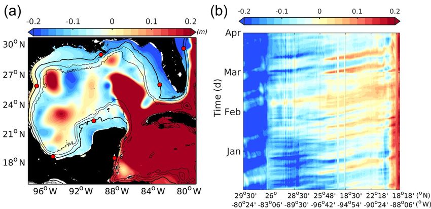
S. N. Estrada-Allis et al.: DIN and PON budget in the Yucatán shelf                                                          1091

component of the TN. The TN cross-shelf fluxes are com-           Gulf of Mexico Coastal Ocean Observing System (GCOOS)
puted for the north, east, south, and west boundaries for both    (https://products.gcoos.org/, last access: January 2017).
the inner and outer shelf, as indicated in the inset in the up-      Although the YS has no rivers, freshwater inputs play
per right corner of Fig. 1a. Accordingly, the total budget is     a key role impacting the local ecosystem (Herrera-Silveira
obtained as the integral over the area of the shelf and over      et al., 2002). These inputs come from SGD linked to the
the depth of the water column for both the inner and outer        “cenotes” ring (sink holes) system inland. The freshwa-
shelves. The budget also includes the loss to denitrification     ter flux, temperature, salinity, and nutrient concentrations
and to burial in the sediments, which are taken into account      for these sources are not well known. Monthly climato-
for the quantification of the TN budget as sinks of nitrogen.     logical values were calculated for the Mexican rivers and
   The initial concentration and boundary conditions at the       SGD systems, using temporally scattered information found
edges of the GoM model domain (Fig. 1a) of the biogeo-            in the literature (e.g. Rojas-Galaviz et al., 1992; Milliman
chemical variables NH4 , Phy, Zoo, Chl, and pools of detri-       and Syvitski, 1992; Poot-Delgado et al., 2015; Conan et al.,
tus are set to a small and positive value of 0.1 mmol N m−3       2016) and a data collection effort within Mexican institutions
following Fennel et al. (2006, 2011) and Xue et al. (2013).       led by Jorge Zavala-Hidalgo (personal communication, Jan-
As mentioned in these references, the model quickly adjusts       uary 2015) and from the GOMEX IV cruise of CINVESTAV
internally to proper variable values within days to weeks.        (Centro de Investigación y Estudios Avanzados in Merida
Moreover, these boundaries are far away from the YS and           Yucatan) within the CIGoM project. During this cruise, a
therefore the fluxes across the inner and outer YS determined     total of 71 profiles of NO3 , potential temperature, salinity,
internally in the model are not impacted by possible incon-       and chlorophyll were collected at standard depths from 2
sistencies at the GoM open boundaries. Given the lack of          to 20 November 2015. The localization of the profiles is
data for Mexican rivers and groundwater fluxes, the same          shown in Fig. 2. Therefore, fluxes from US rivers forcing the
approach is followed for freshwater inputs as also followed       model present inter-annual variability but Mexican freshwa-
by Xue et al. (2013). The biological model parameters used        ter sources only include a climatology due to lack of infor-
in this study are those shown in Table 1 of Fennel et al.         mation (see Appendix B for more details).
(2006), except for the vertical sinking rates which were re-         The nitrogen concentration for freshwater sources is es-
duced about 10 %, to fit the depth of the deep chlorophyll        sentially DIN. For most of the northern rivers (e.g. Missis-
maximum (DCM) observed with the APEX profiling floats             sippi and Atchafalaya), PON is also considered where avail-
(see Fig. A4). The model does not include an explicit com-        able (Fennel et al., 2011; Xue et al., 2013). For the remain-
partment for nitrogen in the form of DON, although it can be      ing freshwater sources, including the SGD system of YS,
included as in the work of Druon et al. (2010), which adds        the PON contribution is set as a constant small value of
semi-labile DOC and DON as state variables to the original        1.5 mmol N m−3 due to lack of data.
Fennel et al. (2006) model. They comment on the difficulties
of validating the model with observations and highlight open
questions even in the definition of both DOC and DON pools        3     Model evaluation for the YS
(see also Anderson et al., 2015). Considering these difficul-
ties and uncertainties, our approach is to use, initially, more   The model dynamics and its biogeochemistry are validated
basic models to understand their capabilities and build and       to guarantee the simulation is able to reproduce basic fea-
employ more comprehensive ones later on; so the inclusion         tures of the observations in the GoM, particularly in the YS.
of DON and/or DOC compartments is left for future studies.        Model statistics including biases of physical and biological
                                                                  variables are computed to have some idea of their impact on
2.3   Freshwater sources                                          the estimation of the TN budget over this shelf. Since this is
                                                                  a basin-scale coupled model, a general evaluation of the re-
Two riverine systems account for 80 % of the freshwater           sults and their statistics is carried out considering sea surface
discharge into the GoM, the Mississippi–Atchafalaya sys-          temperature, mixed-layer depth, mean kinetic energy, surface
tem with 18,000 m3 s−1 and the Usumacinta–Grijalva sys-           chlorophyll, and deep chlorophyll maximum over the whole
tem with 4500 m3 s−1 (Dunn, 1996; Yáñez Arancibia and             Gulf of Mexico with emphasis on the YS. The results are
Day, 2004; Kemp et al., 2016) (see Appendix B). Fresh-            presented in Appendix A.
water contributions to water volume, salinity, temperature,
and DIN concentration are included as grid-cell sources into      3.1    YS in situ data comparison
the model. Apart from the two main systems, a total of
81 freshwater sources are included, taking into account fresh-    Recall that upwelling into the YS is more intense during
water discharges in the Florida, Texas, and Yucatán shelves       spring–summer and weaker in autumn–winter (Ruiz-Castillo
from the years 1978 to 2015. For the US rivers the daily          et al., 2016; Merino, 1997). While the model presents up-
data were obtained from the US Geological Survey (USGS)           welling during all the simulated months, this seasonal be-
(https://www.usgs.gov/, last access: January 2017) and the        haviour is represented in the model climatologies shown

www.biogeosciences.net/17/1087/2020/                                                     Biogeosciences, 17, 1087–1111, 2020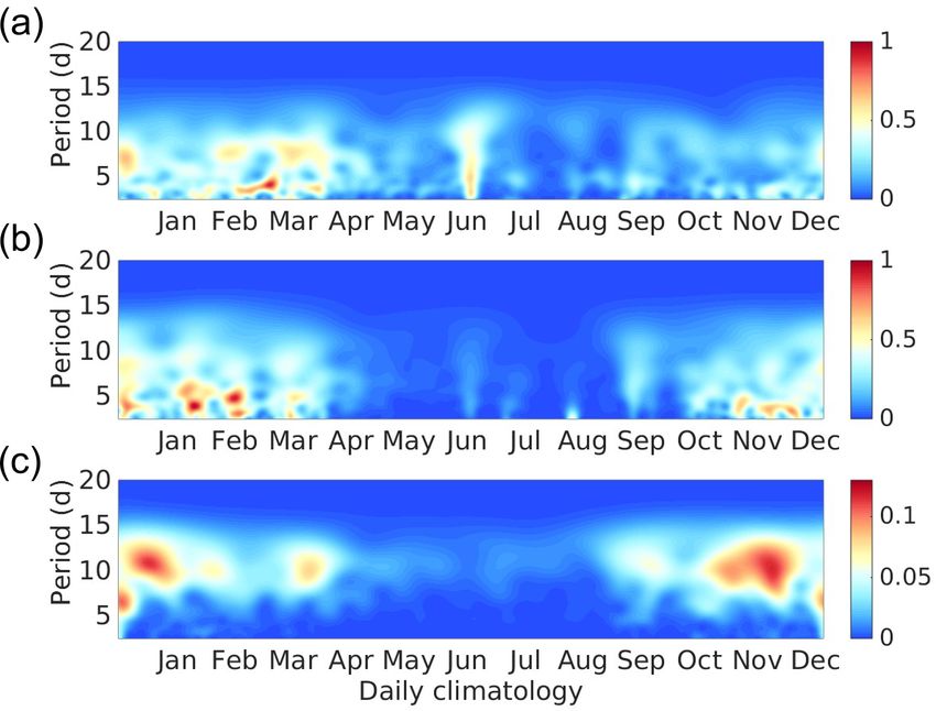
1092                                                         S. N. Estrada-Allis et al.: DIN and PON budget in the Yucatán shelf

Figure 3. Seasonal climatology of bottom temperature (◦ C) for (a) spring and (b) autumn, for the period between 2002 and 2010. The
corresponding vertical sections, indicated by the zonal black line in (a), are shown for (c) spring and (d) autumn. The contours in (a) and (b)
denote the 50 and 250 m isobaths. The black contour in (c) and (d) shows the upwelling isotherm of 22.5 ◦ C.

in Fig. 2. The figure also shows the position of oceano-
graphic stations occupied during the GOMEX IV oceano-
graphic cruise and delimitation of three areas of particular
interest: the inner shelf, the outer shelf, and the upwelling
region at Cape Catoche. The climatology of the YS bottom
temperature (Fig. 3) shows that cold waters enter into the
shelf during spring in agreement with the enhancement of
chlorophyll concentrations (Fig. 2b). The zonal vertical cross
sections show that the isotherm of 22.5 ◦ C, which traces the
upwelled water (Cochrane, 1968; Merino, 1997), outcrops
into the shelf during spring (Fig. 3c). This is not the case in
autumn (Fig. 3d), and the upwelling is weaker (Fig. 2d).
   A point-by-point comparison between the model results
and the in situ observations is shown using only data for
November from 2002 to 2010 in the model, for compatibil-
ity with the observation dates (Figs. 4–7). Since the simula-
tion is for different years, we only expect to reproduce basic
features of these observations. The range of temperatures at
different depths shown by the model agrees well with those
observed during GOMEX IV (Fig. 4). The mean tempera-
ture of the observations is 25.5 ± 2.9 ◦ C, while the model               Figure 4. Comparison between in situ data and simulated temper-
mean temperature is 24.3 ± 3.7 ◦ C. The bias of −1.3 ◦ C is               atures (◦ C). Temperature values correspond to each hydrographic
deemed acceptable considering the model mean is a 9-year                  station, averaged over three depths; (a) between the surface and
mean whereas the mean from observations is from just one                  25 m depth, (b) between 25 and 50 m depth, and (c) between 55 and
month and a different year. A critical area to be evaluated               the deepest measured concentration (z ∼ −150 m). Black dots cor-
                                                                          respond to the observed values and open grey circles to the simula-
is the upwelling region (see dashed box in Fig. 2a), the bias
                                                                          tion. Vertical grey lines are the temporal standard deviation of the
there is −1.1 ◦ C with a root-mean-square error of 1.68 ◦ C.
                                                                          simulated values, as these are temporally averaged over all Novem-
This means that the model tends to be slightly colder than                bers from 2002 to 2010. Vertical black lines delimit the group of
the observations even inside upwelling waters.                            stations for the inner shelf, outer shelf, and upwelling area.
   The model mean salinity is 36.5 ± 0.2, which matches the
36.5 ± 0.2 from observations (Fig. 5). Whilst surface salin-

Biogeosciences, 17, 1087–1111, 2020                                                             www.biogeosciences.net/17/1087/2020/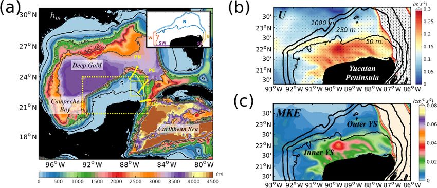
S. N. Estrada-Allis et al.: DIN and PON budget in the Yucatán shelf                                                        1093

Figure 5. Same as Fig. 4, but for salinity.                       Figure 6. Same as Fig. 4, but for chlorophyll concentrations
                                                                  (mg Chl m−3 ).

ity in the model is in relatively good agreement with ob-
servations (Fig. 5a), differences become more important at           To evaluate the temporal behaviour of the model Chl, time
deeper layers (Fig. 5b and c). The root-mean-square error         series of the surface chlorophyll averaged over the shelf are
of model salinity (0.23) as well as the bias (−0.04) is low,      compared to similar time series from satellite surface chloro-
which tends to underestimate the salinity observations. These     phyll from MODIS (see Fig. 8c and Appendix A for a de-
low differences are also found in the bias for the upwelling      scription of the satellite product) during the simulation pe-
area, although the model overestimates the salinity by 0.21       riod. Mean values of satellite surface Chl are 0.38 ± 0.09 and
there. The model is able to represent the main characteristics    0.36 ± 0.13 mg Chl m−3 in the model. Besides reproducing
of the Caribbean Subtropical Underwater coming from the           temporal mean and variability of the surface chlorophyll, the
Caribbean Sea (Merino, 1997) and the Gulf Common Water            model is able to reproduce a positive trend present in the 9
from the GoM (e.g. Enriquez et al., 2013) within the YS. The      years of satellite data. No trend is present in any of the bio-
warm and high-salinity Yucatán Sea Water at the surface de-       geochemical forcings of the model, and determining which
scribed in Enriquez et al. (2013) is present in the model too,    physical mechanisms produce it requires further investiga-
although temperatures do not exceed 31◦ (not shown) as in         tion (see below).
observations.                                                        The simulated nutrient concentration depicts values with
   For Chl, the model results fall within the range ob-           a similar order of magnitude (∼ 3.1 ± 4.6 mmol N m−3 ) as
tained from fluorometer observations in the inner shelf,          the observed profiles (∼ 3.7 ± 5.2 mmol N m−3 ) (Fig. 7).
outer shelf, and upwelling areas (Fig. 6). The mean ob-           Surface nutrient concentrations are underestimated by a
served Chl (0.52 ± 0.58 mg Chl m−3 ) is slightly larger than      1.7 (mmol N m−3 ) compared to observed profiles (Fig. 7a).
the model results (0.44 ± 0.42 mg Chl m−3 ) but within the 1      At subsurface depths (25–55 m), the model tends to under-
standard deviation range, with a bias of −0.08 mg Chl m−3         estimate the NO3 concentrations; however, in the upwelling
and a root-mean-square error of 1.16 mg Chl m−3 . Notice          area, model NO3 concentrations are closer to the observed
that there is agreement in Chl concentration between the          values with a bias of −0.7 mmol N m−3 and larger standard
model and observations in the three layers between 150 m          deviations for both the model (4.0 ± 5.0 mmol N m−3 ) and
depth and the surface (Fig. 6a–c). In the upwelling area the      observations (4.81 ± 6.33 mmol N m−3 ) (Fig. 7b). The tem-
model has lower concentrations than observations with a           poral variability of the modelled NO3 is larger than the ob-
bias of −0.39 mg Chl m−3 and a root-mean-square error of          served NO3 at the surface and bottom as shown by the largest
1.39 mg Chl m−3 ; although the bias is relatively low, it needs   standard deviation in Fig. 7b. Below 55 m the modelled and
to be taken into consideration for the TN budget. Addition-       observed NO3 are in good agreement in both the outer shelf
ally, a comparison with observed mean chlorophyll vertical        and the upwelling area (Fig. 7c). Again, these model re-
profiles over the YS is presented in Fig. A9 of Appendix A.       sults are deemed consistent with observations and are in
Profiles have a similar structure but the model tends to un-      the range of other values reported in the literature (Merino,
derestimate the DCM.                                              1997). Comparison of similar budgets from other shelves in
                                                                  the GoM can be made (e.g. Xue et al., 2013), though clear

www.biogeosciences.net/17/1087/2020/                                                     Biogeosciences, 17, 1087–1111, 2020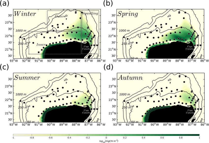
1094 S. N. Estrada-Allis et al.: DIN and PON budget in the Yucatán shelf
Figure 7. Same as Fig. 4, but for nitrate concentrations
(mmol N m−3 ).
interpretation of similarities and differences between them
may be difficult given the differences in dynamics and nitrate
sources and sinks controlling the budgets on each shelf. One
could easily compute budgets per unit area or length for a
more sensible comparison among different shelves but in the
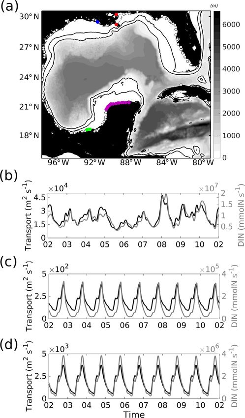
Figure 8. Temporal series of TN (thick black line), DIN (thin
literature only total budgets are available (see Table 2 in Xue black line), and DIN (thin grey line) in millimoles of nitrogen,
et al., 2013). In that regard, the inner and outer shelf areas are spatially integrated over (a) the inner shelf and (b) the outer
∼ 74 and ∼ 91 km2 , respectively. The TN concentrations for shelf. Panel (c) shows the temporal series from monthly satel-
each shelf can be extracted by averaging over the 9-year sim- lite chlorophyll (black, mg Chl m−3 ) and from the model outputs
ulation the integrated values of Fig. 8, with 14.6±0.83×10¹⁶ (grey) averaged over the whole Yucatán shelf. Dashed thick lines
and 7.42 ± 0.89 × 10¹⁶ mmol N, for the inner and outer shelf, are the trend indicated by the linear fit for the TN or chloro-
respectively. phyll time series, where thinner dashed lines are the respective
In addition, the model sea level elevation and surface 95 % confidence intervals. Equations of each linear fit are TN (in-
ocean currents are compared against altimeter products in ner shelf) = 2.33 × 10¹² d + 4.2 × 10¹⁶ , TN (outer shelf) = 2.40 ×
1012 d + 7.0×10¹⁶ , Chl (satellite) = 0.0010 months + 0.28, and Chl
Appendix A, where YC variability and transport from the
(model) = 0.0010 months + 0.30. Notice that the trend is positive
model are compared with data from three moorings located
for all the temporal series.
on the slope close to the eastern YS rim described in Shein-
baum et al. (2016).
This is an interesting problem currently under investigation
and to be reported elsewhere.
In the inner shelf there are similar total integrated values
4 TN budget and cross-shelf transports in the YS
of DIN and PON (Fig. 8a). This indicates the presence of a
very “efficient” biogeochemical cycle in the inner shelf (see
Time series of spatially averaged TN over the YS suggest a
explanation below). By contrast, in the outer shelf, DIN val-
positive trend over the 9 simulated years. The trend is seen
ues are larger than PON (Fig. 8b) probably because the in-
in both the inner and the outer shelves (Fig. 8a and b). This,
tegration in the outer shelf includes a large volume below
perhaps, could be expected given the positive trend in both
the euphotic zone. Temporal series of integrated TN show a
model and satellite surface Chl mentioned before (Fig. 8c).
combination of low-frequency variability associated with the
Varela et al. (2018) report a cooling trend of the inner YS and
seasonal cycle as well as interannual variability, but longer
suggest it may be associated with an eastward shift of the YC.
period integrations are required to properly investigate the
We searched for possible connections between the trends in
latter.
chlorophyll and TN and indices measuring the position and
strength of the YC in the model but found no correlation.
Biogeosciences, 17, 1087–1111, 2020 www.biogeosciences.net/17/1087/2020/
S. N. Estrada-Allis et al.: DIN and PON budget in the Yucatán shelf 1095
Table 1. Nutrient budget in moles of nitrogen per year for the inner
(50 m isobath) and outer (250 m isobath) Yucatán shelf, computed
at each boundary (N, W, E, and S; see Fig. 1a) using cross-shelf ve-
locities. The flux of nutrients is integrated through the water column
and temporally averaged using the period 2002–2010 to compute
the budget from daily model fields. Positive (negative) values repre-
sent sources (sinks) of nutrients. Denitrification is always a nitrogen
removal process.
Boundary PON DIN TN Fresh
water/
innera
Inner-shelf budget (×1010 mol N yr−1 )
N 0.34 1.63 1.97 0.76
W −0.72 −0.02 −0.73 0.72
E 2.35 1.68 4.32 0
S −2.29 −0.05 −2.34 0
Denitrification −3.34
Trendb −0.64
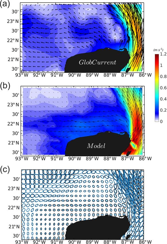
Figure 9. Scheme of the TN budget for the Yucatán shelf. Black and
white arrows denote cross-shelf flux for the outer and inner shelf, re- Outer-shelf budget (×1010 mol N yr−1 )
spectively. In blue is the PON, in red the DIN, in green the freshwa-
ter DIN sources (Rivers), and in yellow the sinks of TN due to den- N −11.46 −7.42 −18.88 −1.97
itrification (DNF). The values are expressed in mol N yr−1 × 10¹⁰ . W −1.85 −9.87 −11.72 0.72
Negative values indicate sink, whereas positive indicates a source E −0.28 7.65 7.36 −4.03
of TN. The isobaths that delimit the inner (50 m depth) and outer S 11.17 27.74 38.92 0
(250 m depth) shelves are also highlighted. Denitrification −3.34
Trendb −0.66
a Freshwater sources are considered only for the inner shelf. Inner can be taken
as a source or sink of nitrogen only for the outer shelf. b The positive trend of
To understand the high TN variability in the YS, quan- total nitrogen observed in the temporal series during 9 years is also taken into
tification of the cross-shelf fluxes becomes necessary. Their consideration to close the budget.
impact on the TN budget and the physical mechanisms mod-
ulating such fluxes are investigated next.
Cross-shelf fluxes are quantified for the two compart- hanced during winter, when vertical wind-driven mixing and
ments, the inner and outer shelves (Fig. 1b), and for all the convective processes are strong enough to reach the sea bot-
boundaries of each compartment. A schematic view of the tom. Additionally, vertical shear likely generated by bottom
main incoming and outgoing pathways of cross-shelf TN friction can lead to instabilities and vertical mixing able to
fluxes is shown in Fig. 9. The yearly averages of the spatially break the stratification and carry nutrients to the euphotic
integrated cross-shelf fluxes are shown in Table 1. zone. During summer months, vertical mixing is weaker (not
For the inner shelf, both PON and DIN are imported shown). Turns out that, in the model, vertical velocities in
through its northern and eastern boundaries and exported the inner shelf are quite intense and upward throughout the
through the west and south borders. The inner shelf acts as year (∼ 5 m d−1 ), carrying nutrients to the euphotic layer.
a source of PON for the Campeche Bay at the southwest The cause of these vertical velocities is under investigation
margin. The major source of TN for the inner shelf is from using a higher-resolution model configuration.
the outer shelf via the Cape Catoche upwelling, represent- By contrast, in the outer shelf, the largest inputs of PON
ing 80 % of the total, while freshwater sources contribute the and DIN are advected from its southeastern corner. The east-
other 20 %. Although the latter is a relatively large source of ern boundary is a source of DIN but a sink of PON for the
nitrogen, its relevance seems to be confined to the NW part of outer shelf. Therefore, the budget reveals that the PON ex-
the inner shelf. In general, there is compensation between the ported to the inner shelf is produced in the outer shelf and
DIN and PON concentrations in the inner shelf (Fig. 8a) due not advected from Caribbean waters. The contribution of TN
to an efficient biogeochemical cycle whereby almost all the from the inner shelf to the outer shelf represents only 1.5 %
DIN imported into the shelf is consumed by the phytoplank- of the total inputs.
ton and thus converted into PON. The efficiency relies on Over the outer shelf the fluxes of nutrients and organic
the shallowness of the inner shelf (∼ 50 m depth), because, matter are driven by a westward wind-driven circulation
if strong mixing conditions are present, organic matter will (Ruiz-Castillo et al., 2016) and exported to the deep GoM
distribute throughout the shallow water column. This is en- and the Campeche Bay through the north and west borders,
www.biogeosciences.net/17/1087/2020/ Biogeosciences, 17, 1087–1111, 2020
1096                                                     S. N. Estrada-Allis et al.: DIN and PON budget in the Yucatán shelf

respectively. This represents a source of DIN, Phy, and Zoo        upwelling pulses. In this study, the presence of CTWs is cor-
to these oligotrophic regions.                                     roborated and its effect on the modulation of cross-shelf nu-
   In that regard, the model reveals a quasi-permanent thin        trient fluxes at the west margin of the YS is exposed.
filament of Chl that is advected from the northwest corner of         The presence of CTWs in the model simulations is ev-
the outer shelf to the west of the Campeche Bay (Fig. 10a).        idenced in the Hovmöller diagram along the 50 m isobath
A vertical section of the cross-shelf fluxes along the 250 m       shown in Fig. 11. Phase speeds are in the range of [2–
isobath in the western YS (TN, Fig. 10b) shows that while          4] m s−1 in agreement with observations (Dubranna et al.,
the export of organic matter to the open sea is concentrated       2011) and other models (Jouanno et al., 2016).
in the surface layers (Fig. 10d), the bottom layer presents a         The cross-shelf TN in the YS western inner-shelf bound-
net DIN export (Fig. 10c). The climatological average over         ary exhibits high-frequency variability. The daily climatol-
9 years of simulated Chl shows that this filament is intensi-      ogy of the wavelet power spectrum of wind stress, sea level
fied during winter (not shown), although it is present during      anomaly (SLA), and western boundary cross-shelf TN tem-
the whole simulation period. Sanvicente-Añorve et al. (2014)       poral series for the inner shelf of Fig. 12 show that both
studied the larval dispersal for coral reef ecosystems in the      along-shelf wind stress and changes in SLA may be linked
southern GoM. They show that the northwestern corner of            with the cross-shelf TN variability in the inner shelf. The
the outer YS acts as a sink region for larvae. Similar to other    three variables show maximum energy during winter times
coral reef systems, they attributed the sink to the influence      when CTWs are expected to be more intense, and the wind
of circulation patterns that lead to a unidirectional dispersion   increases its magnitude due to the incursion of the “Nortes”
pattern during the whole year. Our model results seem to sup-      (cold front winds).
port this idea.                                                       It is worth mentioning that the wavelet power spectrum for
   Denitrification is a form of anaerobic microbial respira-       the whole 2002–2010 period (not shown) depicts an interest-
tion in which nitrate and nitrite are finally reduced to molec-    ing intensification of cross-shelf flow (and nutrient fluxes)
ular nitrogen (N2 ). It represents a major sink for bioavailable   during 2003, 2004, 2009, and 2010 which coincides with
nitrogen. The spatio-temporal average rate of denitrification      El Niño Modoki events (Ashok et al., 2007; Ashok and Ya-
for the YS is 1.11 ± 0.13 mmol N m−2 d−1 . Our results sug-        magata, 2009). The possibility of such a connection deserves
gest that denitrification removes up to the 53 % of the TN         further investigation.
in the inner shelf, a significant percentage that agrees with         To further examine the relationship between these phys-
estimates from other shelves in the GoM (Xue et al., 2013).        ical and biogeochemical variables, results from a cross-
On the other hand, denitrification in the outer shelf only re-     correlation spectral analysis are shown in Fig. 13 for the time
moves 9 % of the TN. Our results also indicate that deni-          series used in the wavelet analysis of Fig. 12. The variability
trification rates tend to increase with time for both inner and    of along-shelf wind stress and cross-shelf TN fluxes shows
outer shelves (not shown), in concert with TN concentrations       significant coherence in the 8–10 d period band at nearly
(Fig. 8a and b). This is expected since denitrification is a re-   zero phase lag (Fig. 13). Coherence between cross-shelf TN
duction process; hence an increase in nitrate concentration        fluxes and SLA is also coherent in the same band (peaks at
means more available DIN to be reduced to N2 .                     8 and 8.4 d) but 180◦ out of phase. This is consistent with
                                                                   offshore Ekman transport produced by along-shelf northerly
4.1    Physical modulation of cross-shelf TN flux                  winds triggering nutrient and organic matter fluxes across the
       by CTWs                                                     western boundary of the YS and negative SLA at the coast.
                                                                      Propagation of CTWs is evident in the Hovmöller diagram
Many physical process coexist at different spatio-temporal         of Fig. 11 and most certainly modulates the cross-shelf TN
scales in the YS that modulate the cross-shelf transport of        transport. The coherent 8–10 d period band (and also at other
nutrients and organic matter. We suggest that at least two         higher frequencies, e.g. 5–6 d period) is in agreement with
processes are responsible for such modulation: CTWs and            those reported in the literature for CTWs in the GoM (e.g.
interaction of the YC with the eastern shelf break.                Jouanno et al., 2016). Since the coherence analysis is car-
   CTWs can be generated by wind forcing over irregular            ried out here using time series of spatially averaged quanti-
bottom topography along the coast and have been the subject        ties (from 20◦ 300 N to almost 22◦ N, approximately 100 km),
of investigation for a long time (e.g. Clarke, 1977). In the       possible phase lags are probably masked.
GoM, CTWs are forced by alongshore winds and then travel
anticlockwise with the coast on its right until they reach the     4.2   Influence of the Yucatán Current in the coastal
western portion of the Yucatán Peninsula, mainly associated              upwelling
with cold fronts (Dubranna et al., 2011; Jouanno et al., 2016).
CTWs have a signature in sea level that is well captured in        Observational studies suggest that favourable-upwelling
relatively high-resolution models such as the one used in the      winds at the northern Yucatán coast are present all year round
present study (∼ 5 km). In their modelling study, Jouanno          (Ruiz-Castillo et al., 2016; Pérez-Santos et al., 2010). Cold
et al. (2018) suggest that CTWs may influence the Yucatán          SSTs on the YS vary seasonally and are particularly charac-

Biogeosciences, 17, 1087–1111, 2020                                                    www.biogeosciences.net/17/1087/2020/
S. N. Estrada-Allis et al.: DIN and PON budget in the Yucatán shelf 1097 Figure 10. (a) Map of surface chlorophyll (mg Chl m−3 ), averaged over the 9 simulated years. The three characteristic isobaths are de- noted. A total of 9 years of averaged cross-shelf fluxes along the 250 m isobath at the western boundary of (b) TN, (c) DIN, and (d) PON (mmol N m−2 s−1 ). Negative values indicate westward flux, i.e. TN flux from the shelf to the Campeche Bay. The area delimited by dashed lines shows the location of the filament depicted in (a), in the NW of the YS. Figure 11. (a) Snapshot of sea level anomaly (η, m) for the simulated year 2005. (b) Hovmöller diagram of η along the 50 m isobath from January to April of the year 2005. Red dots in (a) denote the latitude and longitude shown at the bottom of (b), from Florida to the Yucatán Peninsula. terized by a cold water band on the inner YS very close to the ration and/or encroachment from the coast, bottom bound- coast that appears in spring and continues until the beginning ary layer transport, advection, instabilities, eddies, and the of autumn (Ruiz-Castillo et al., 2016; Zavala-Hidalgo et al., presence of particular topographic features (e.g. submarine 2006). Pérez-Santos et al. (2010), using 10 years of sea sur- canyons. The reader is referred to Roughan and Middleton face wind data from QuikSCAT, show that Ekman transport (2002) for a discussion of upwelling mechanisms on the East is the main contributor to the upwelling over the north YS Australian Current that appear to be relevant here too as sev- (93 %), with Ekman pumping only contributing 7 %. eral local studies indicate (Cochrane, 1966; Merino, 1997; This upwelling regime requires a supply of cold and Zavala-Hidalgo et al., 2006; Enriquez et al., 2010, 2013; En- deeper nutrient-rich waters from the open ocean to maintain riquez and Mariño Tapia, 2014; Carrillo et al., 2016; Jouanno the observed biological productivity on the YS. et al., 2016, 2018). The main import of TN to the YS is through the southeast On the other hand, the export of TN to the deep GoM and eastern YS boundaries via mechanisms related to the dy- through the YS northern margin can also be related to advec- namics of the Yucatán and Loop currents and their interac- tion by the YC and associated mesoscale structures (Roughan tion with the YS shelf break, such as intensification, sepa- www.biogeosciences.net/17/1087/2020/ Biogeosciences, 17, 1087–1111, 2020
1098                                                          S. N. Estrada-Allis et al.: DIN and PON budget in the Yucatán shelf

                                                                         Figure 14. Temporal series for the 9 simulated years of cross-shelf
                                                                         Yucatán Current component (YC), total nitrogen (TN), dissolved
                                                                         inorganic nitrogen (DIN), and particulate organic nitrogen (PON),
                                                                         vertically integrated and averaged over the isobath 250 m of the
                                                                         eastern boundary. The square of the correlation coefficients (r 2 ),
Figure 12. Wavelet power spectrum for time series averaged over          between YC and the biogeochemical variables, is shown at the top.
the western 50 m isobath of (a) cross-shelf total nitrogen flux ver-     The temporal series are filtered by a moving average of 30 d to re-
tically integrated (TN, mmol N m−1 s−1 ), (b) along-shelf wind           move daily variability.
stress (τalong , N m−2 ), and (c) sea level anomaly (SLA, m). The
temporal series are detrended, normalized, and filtered by a Lanc-
zos high-pass filter with a cut-off of 15 d.
                                                                         and Middleton, 2002; Carrillo et al., 2016; Enriquez and
                                                                         Mariño Tapia, 2014).
                                                                            Correlation analysis between the strength of the cross-
                                                                         shelf flow from the YC, PON, and DIN fluxes at the eastern
                                                                         margin, all vertically integrated, shows high values at sea-
                                                                         sonal timescales (Fig. 14). The time series are filtered by a
                                                                         30 d moving-average window to remove high-frequency vari-
                                                                         ability. The square of the correlation coefficients (r 2 ) for DIN
                                                                         and PON against the vertically integrated YC is indicated at
                                                                         the top of Fig. 14. These results indicate that TN fluxes are
                                                                         well correlated with the strength of the current.
                                                                            To investigate the possible role of the position and tra-
                                                                         jectory of the YC and its closeness to the YS in the up-
                                                                         welling (Enriquez et al., 2010, 2013; Jouanno et al., 2018),
                                                                         we computed an index measuring the closeness of the YC
                                                                         core to Cape Catoche and the notch areas in the model, which
                                                                         are two places where water tends to upwell (Merino, 1997;
                                                                         Jouanno et al., 2018). The index depicts no seasonality that
                                                                         could be directly connected to strong(weak) upwelling dur-
Figure 13. (a) Cross-correlation spectral analysis of time se-           ing spring (autumn). This is an indication that seasonality
ries over the western 50 m isobath, indicating the square coher-         of the inflow of nutrient-rich water into the YS is probably
ence coefficient between along-shelf wind stress (τalong , N m−2 )       more influenced by other processes as discussed in Reyes-
and cross-shelf total nitrogen flux vertically integrated (TNcross ,
                                                                         Mendoza et al. (2016), such as cold front winds that can stop
mmol N m−1 s−1 ) in black and between sea level anomaly
                                                                         the upwelling or other non-local perturbations.
(SLA, m) and TNcross in grey. The black horizontal line indicates
the 95 % confidence interval. Analysis for the 9 simulated years            One of the important mechanisms suggested since
based on daily outputs with a 30 d window. Before analysis, the          Cochrane (1966) to be responsible for the YS eastern bound-
temporal series are detrended, normalized, and filtered by a Lanc-       ary upwelling and the nutrient flux towards the coast is bot-
zos high-pass filter with a cut-off of 15 d. Panel (b) shows the phase   tom Ekman layer transport produced by interaction of the YC
or anti-phase in degrees of both coherence analysis of (a) τalong and    with the upper slope and shelf break. The stress exerted by
TNcross in black and SLA and TNcross in grey.                            the intense along-shore velocity of the YC on the topography
                                                                         generates an Ekman spiral at the bottom boundary layer and
                                                                         a net depth integrated transport to the left, i.e. a cross-shelf
                                                                         transport towards the shelf in the boundary layer. For exam-

Biogeosciences, 17, 1087–1111, 2020                                                            www.biogeosciences.net/17/1087/2020/
S. N. Estrada-Allis et al.: DIN and PON budget in the Yucatán shelf 1099
ple, Shaeffer et al. (2014) using glider observations find that summer. This bias produces more intense upwelling at Cape
bottom Ekman transport can explain up to the 71 % of the Catoche during spring than in summer. In fact, upwelling wa-
bottom cross-shelf transport variability on the southeastern ters are still present during winter (Fig. 2) but not in obser-
Australian shelf produced by the East Australian Current. vations. The filtered seasonal time series of bottom Ekman
Here we present modelling evidence that bottom Ek- transport shown in Fig. 15b (black line) depict the same pat-
man layer transport could be the precursor of the up- tern: they indicate that water from the Caribbean Sea entering
welling in Cape Catoche. The bottom Ekman transport (UbE , into the YS (via bottom Ekman transport) increases during
m2 s−1 ) can be taken as UbE = −τby /(ρo f ), q where τby is spring towards the summer, decreases during autumn, and in-
the bottom stress computed by τby = ρo Cdvb u2b + vb2 , with creases again during winter. This is in agreement with Fig. 3.
In the water column, the model underestimates NO3 con-
Cd=1×10⁻³ as the drag coefficient, ub and vb the bottom centration a maximum of 15 % and is also about 5 % colder
velocities at the 250 m isobath, f the Coriolis frequency, than the observed vertical profiles. These biases can impact
and ρo = 1025 kg m−3 the reference potential density of the the growth of phytoplankton whose maximum growth rate
sea water. The analysis shows that the time-mean UbE is (Eppley, 1972) depends on temperature and nutrient concen-
toward the shelf (defined positive here), and is well corre- tration (Fennel et al., 2006). However, since phytoplankton
lated with the bottom cross-shelf water transport (r 2 = 0.71, only represent 15 % of the TN, the overall impact on TN of
ci = 95 %) calculated directly (Fig. 15a). The Ekman trans- these biases is estimated to be less than 3 %. The main point
port is calculated from the theoretical formula (i.e. stress di- we are trying to make is that, although there are model bi-
vided by the coriolis frequency), whereas the direct transport ases, the main processes that control the TN budget in the YS
is calculated using the bottom velocities and integrating on are well captured by the model simulation, particularly the
the last grid cell. We should mention here that the bottom Cape Catoche upwelling, which together with the southeast-
grid cell at this depth has a vertical size of ∼ 20 m. Using ern boundary represent the main entrance of TN to the YS.
standard formulas to estimate the width of the Ekman layer
(e.g. Cushman-Roisin and Beckers, 2011; Perlin et al., 2007)
from bottom velocities or stresses and stratification, we ob- 6 Summary and concluding remarks
tain values ∼ 10–30 m. Therefore the layer is not really re-
solved by the model grid. The correlation is also large over The TN budget, the main nutrient transport pathways and
time (r 2 = 0.78, ci = 95 %) as shown in Fig. 15b. Figure 15c their modulation by physical processes over the Yucatán
shows that the vertically integrated TN transport averaged shelf have been investigated using a 9-year simulation from
over 9 simulated years and over latitude is towards the coast a ROMS physical–biogeochemical coupled model for the
at 250 m depth, that is, at the bottom-most model layer which GoM. Our work provides a first general view of the shelf
is considered here to be the bottom Ekman layer. physical–biogeochemical coupled system, schematized in
Comparison between bottom-layer Ekman transport and Fig. 16.
the time mean vertically integrated TN transport across the The results indicate that TN, especially DIN, enters the
eastern 250 m isobath indicates that bottom Ekman transport Yucatán outer shelf through the southeastern and eastern
is responsible for 65 % of the TN that is entering the shelf. margins. The TN is then driven by a westward shelf cur-
The mechanisms that explain the remaining flux need to be rent and then exported to the deep GoM and Campeche Bay
further investigated and are probably related to meanders, through the northern and western boundaries, respectively.
eddies, topographic features, and other processes. Moreover, In the inner shelf, the biogeochemical nitrogen-based cycle
bottom Ekman transport can be arrested by stratification and seems to be very efficient for NO3 remineralization and con-
may not be dominant everywhere along the YS east coast as sumption by the phytoplankton, converting most of the DIN
has been documented in other western boundary upwelling to PON. The freshwater sources represent an important con-
regions (e.g. Roughan and Middleton, 2002, 2004). Our goal tribution of about 20 % to the DIN concentration, although it
here was only to estimate the size of the TN fluxes related is restricted to the northwest of the Yucatán Peninsula. Den-
to the bottom Ekman layer and determine its relative impor- itrification represents the main sink of nutrients for the inner
tance. shelf, removing more than the 50 % of the nitrogen. The in-
ner shelf contributes to the TN of the outer shelf at its west-
ern edge, but this contribution is less than 2 %, indicating
weak fluxes from the inner to the outer Yucatán shelf. By
5 Model uncertainties
contrast, the outer shelf is the main nitrogen supplier of the
inner shelf, particularly of PON from the eastern margin. A
The bias of the model with respect to observations described
quasi-constant filament in the outer shelf western border rep-
in Sect. 3 (see also Appendix A) is analysed in order to exam-
resents an important source of both organic and inorganic
ine how uncertainties may impact the TN budget calculation.
nitrogen for the oligotrophic Campeche Bay.
The model tends to overestimate (underestimate) Chl
(SST) in winter and underestimate (overestimate) Chl (SS) in
www.biogeosciences.net/17/1087/2020/ Biogeosciences, 17, 1087–1111, 20201100 S. N. Estrada-Allis et al.: DIN and PON budget in the Yucatán shelf
Figure 15. Flux of TN (QTN ) computed by the bottom Ekman transport (UbE , m2 s−1 ) for the 9 simulated years (blue) compared with the
bottom-most layer TN flux (grey, mmol N m−1 s−1 ) over the Ekman bottom layer for (a) temporal averages and (b) spatial averages over the
250 m isobath, where the superimposed black line is the bottom Ekman transport filtered with a 90 d moving average. (c) Vertically integrated
TN flux along the eastern 250 m isobath, averaged over latitude and over the 9 simulated years in mmol N m−1 s−1 . Shaded areas denote the
standard deviation of the averages.
correlated with changes in SLA at similar periods, which
are also typical of CTWs found in the GoM. Coherence is
180◦ out of phase and consistent with negative SLA result-
ing from offshore Ekman transport. These exchanges are en-
hanced during winter due to cold frontal atmospheric systems
Nortes.
The advection by the YC dominates the nutrient concen-
tration import to the YS through the southeastern border. This
advection, together with the influence of mesoscale struc-
tures, control the export of nutrients to the deep GoM at the
northern margin. A different process modulates the flux of
nutrients at the eastern YS margin. The YC flowing paral-
lel to the slope plays an important role in the intrusion of
DIN into the shelf. Initial estimates carried out in this study
suggest that, in the model, bottom Ekman layer transport ex-
plains the deep TN flux through the eastern YS boundary.
There is a positive mean transport (into the shelf) over the
9 simulated years along the eastern shelf break so friction
generated between the YC and the shelf break produces a
Figure 16. Schematic view of the main physical processes that net bottom Ekman transport towards the shelf. This produces
modulate the cross-shelf transport of TN in the Yucatán shelf.
the upwelling at Cape Catoche on the eastern shelf, but it is
not the only process at work: external and remote forcings
appear to control its seasonality (e.g. winds, CTWs); in ad-
Surface Ekman layer dynamics at the western and north- dition, other upwelling mechanisms such as divergence and
western shelf borders play an important role in the transport convergence from current separation and encroachment and
of nutrient and organic matter to the Campeche Bay and deep eddy-current interactions with topographic features (e.g. sub-
central GoM. Part of the high-frequency variability of the marine canyons) may be important too and must be analysed
TN fluxes at the western YS boundary are correlated and in in future research.
phase with the along-shelf wind-stress modulating the vari-
ability of TN across the western shelf of the Yucatán in the
5–10 period band. These high-frequency TN fluxes are also
Biogeosciences, 17, 1087–1111, 2020 www.biogeosciences.net/17/1087/2020/You can also read