From climatological to small-scale applications: simulating water isotopologues with ICON-ART-Iso (version 2.3)
←
→
Page content transcription
If your browser does not render page correctly, please read the page content below
Geosci. Model Dev., 11, 5113–5133, 2018
https://doi.org/10.5194/gmd-11-5113-2018
© Author(s) 2018. This work is distributed under
the Creative Commons Attribution 4.0 License.

From climatological to small-scale applications: simulating water
isotopologues with ICON-ART-Iso (version 2.3)
Johannes Eckstein1 , Roland Ruhnke1 , Stephan Pfahl2,3 , Emanuel Christner1 , Christopher Diekmann1 ,
Christoph Dyroff1,a , Daniel Reinert4 , Daniel Rieger4 , Matthias Schneider1 , Jennifer Schröter1 , Andreas Zahn1 , and
Peter Braesicke1
1 Karlsruhe Institute of Technology (KIT), Institute of Meteorology and Climate Research (IMK),
Herrmann-von-Helmholtz-Platz 1, 76344 Eggenstein-Leopoldshafen, Germany
2 ETH Zürich, Institute for Atmospheric and Climate Science, Universitätstrasse 16, 8092 Zürich, Switzerland
3 Freie Universität Berlin, Institute of Meteorology, Carl-Heinrich-Becker-Weg 6-10, 12165 Berlin, Germany
4 Deutscher Wetterdienst, Frankfurter Str. 135, 63067 Offenbach, Germany
a now at: Aerodyne Research Inc., 45 Manning Road, Billerica, MA 01821, USA

Correspondence: Johannes Eckstein (johannes.eckstein@kit.edu)

Received: 2 November 2017 – Discussion started: 20 December 2017
Revised: 26 October 2018 – Accepted: 29 November 2018 – Published: 14 December 2018

Abstract. We present the new isotope-enabled model ICON-          eral features of this sample as well as those of all tropical data
ART-Iso. The physics package of the global ICOsahedral            available from IAGOS-CARIBIC are captured by the model.
Nonhydrostatic (ICON) modeling framework has been ex-                The study demonstrates that ICON-ART-Iso is a flexible
tended to simulate passive moisture tracers and the stable        tool to analyze the water cycle of ICON. It is capable of sim-
isotopologues HDO and H18     2 O. The extension builds on the    ulating tagged water as well as the isotopologues HDO and
infrastructure provided by ICON-ART, which allows for high        H18
                                                                    2 O.
flexibility with respect to the number of related water tracers
that are simulated. The physics of isotopologue fractionation
follow the model COSMOiso. We first present a detailed de-
scription of the physics of fractionation that have been im-      1   Introduction
plemented in the model. The model is then evaluated on a
range of temporal scales by comparing with measurements           Water in gas, liquid and frozen form is an important com-
of precipitation and vapor.                                       ponent of the climate system. Ice caps and snow-covered
   A multi-annual simulation is compared to observations of       surfaces strongly influence the albedo of the surface (Kraus,
the isotopologues in precipitation taken from the station net-    2004), the oceans are unmatched water reservoirs, which dis-
work GNIP (Global Network for Isotopes in Precipitation).         solve trace substances (Jacob, 1999) and redistribute heat
ICON-ART-Iso is able to simulate the main features of the         (Pinet, 1993), and all animal and plant life depends on liq-
seasonal cycles in δD and δ 18 O as observed at the GNIP sta-     uid water. The atmosphere is by mass the smallest compart-
tions. In a comparison with IASI satellite retrievals, the sea-   ment of the hydrological cycle, but it is this compartment
sonal and daily cycles in the isotopologue content of vapor       that serves to transfer water between the spheres of liquid,
are examined for different regions in the free troposphere.       frozen and biologically bound water on the earth’s surface
On a small spatial and temporal scale, ICON-ART-Iso is            (Gat, 1996). For atmospheric processes themselves, water is
used to simulate the period of two flights of the IAGOS-          also of great importance. It is the strongest greenhouse gas
CARIBIC aircraft in September 2010, which sampled air in          (Schmidt et al., 2010) and distributes energy through the re-
the tropopause region influenced by Hurricane Igor. The gen-      lease of latent heat (Holton and Hakim, 2013), while liquid
                                                                  and frozen particles influence the radiative balance (Shine
                                                                  and Sinha, 1991).

Published by Copernicus Publications on behalf of the European Geosciences Union.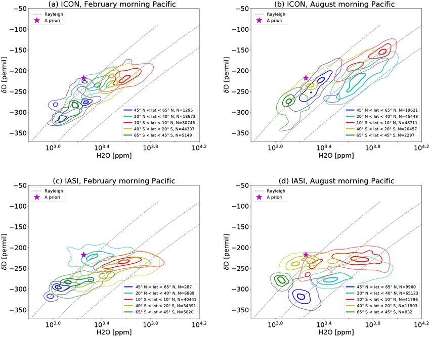
5114                                                  J. Eckstein et al.: Simulating water isotopologues with ICON-ART-Iso

   A correct description of the atmospheric water cycle is         overview), ICON-ART-Iso stands out because of its non-
therefore necessary for the understanding and simulation of        hydrostatic base model core, enabling simulations with fine
the atmosphere and the climate system (Riese et al., 2012;         horizontal resolution on a global grid. Its flexible design al-
Sherwood et al., 2014). The stable isotopologues of water          lows for the simulation of diagnostic evaporation tracers as
are unique diagnostic tracers that provide a deeper insight        well as the isotopologues HDO and H18      2 O during a single
into the water cycle (Galewsky et al., 2016). Because of the       simulation.
larger molar mass of the heavy isotopologues, their ratio to          This article first gives some technical details on ICON and
(standard) water is changed by phase transitions. This change      ICON-ART. This is followed by a detailed description of the
in the ratio is termed fractionation. Considering the isotopo-     physics special to ICON-ART-Iso, which have been imple-
logue ratio of the heavy isotopologues in vapor and precip-        mented in ICON to simulate isotopologues (Sect. 2).
itation (liquid or ice) provides an opportunity to develop an         The remaining sections describe model results and first
advanced understanding of the processes that shape the water       validation studies: Sect. 3.1 looks at passive moisture trac-
cycle.                                                             ers. Focus is laid on the source regions – ocean or land
   Pioneering research on measuring the heavy isotopologues        – of the water that forms precipitation. The next section
of water started in the 1950s and first examined the iso-          (Sect. 3.2) compares data from a simulation spanning more
topologues in precipitation (Dansgaard, 1954, 1964). The-          than 10 years on a coarse grid to measurements from dif-
oretical advances on the microphysics (Jouzel et al., 1975;        ferent stations of the GNIP network. A further validation
Jouzel and Merlivat, 1984) and surface evaporation (Craig          with measurements is performed in Sect. 3.3. Retrievals from
and Gordon, 1965) enabled the implementation of heavy              IASI satellite measurements are compared with ICON-ART-
isotopologues in global climate models (Joussaume et al.,          Iso results for 2 weeks in winter and summer 2014, con-
1984; Joussaume and Jouzel, 1993). Since then, measure-            sidering the seasonal and daily cycle in different regions.
ment techniques and modeling of the isotopologues have ad-         Section 3.4 then discusses the comparison with IAGOS-
vanced. Measurements of the isotopic content of vapor first        CARIBIC measurements. In situ data from two flights are
required cryogenic samplers (Dansgaard, 1954), but in the          compared with results of ICON-ART-Iso simulations. Sec-
last 15 years laser absorption spectroscopy has made in situ       tion 4 summarizes and concludes the study.
observations possible (Lee et al., 2005; Dyroff et al., 2010).
Today, the isotopologue content in atmospheric vapor can
also be derived from satellite measurements (Gunson et al.,        2     The model ICON-ART-Iso
1996; Worden et al., 2006; Steinwagner et al., 2007; Schnei-
der and Hase, 2011). Many global and regional circulation          This section presents the technical and physical background
models have been equipped to simulate the atmospheric iso-         of the model ICON-ART-Iso. First, ICON and the extension
topologue distribution, focusing on global-scale (Risi et al.,     ICON-ART are introduced. Next, general thoughts on sim-
2010; Werner et al., 2011) or regional phenomena (Blossey          ulating a diagnostic water cycle are presented. Starting in
et al., 2010; Pfahl et al., 2012, both limited-area models). De-   Sect. 2.3, the main processes that influence the distribution of
spite this progress, the potential of isotopologues to improve     the isotopologues are discussed in separate sections: surface
the understanding and physical description of single pro-          evaporation, saturation adjustment, cloud microphysics and
cesses “remains largely unexplored” (Galewsky et al., 2016).       convection. To close this technical part, Sect. 2.7 discusses
A more extensive literature overview on the subject is given       the initialization of the model.
by Galewsky et al. (2016).
   We present ICON-ART-Iso, the newly developed,                   2.1    Introduction to the modeling framework
isotopologue-enabled version of the global ICOsahedral                    ICON-ART
Nonhydrostatic (ICON) modeling framework (Zängl et al.,
2015). By design, ICON is a flexible model capable of              ICON-ART-Iso is the isotope-enabled version of the model
simulations from climatological down to turbulent scales           ICON. ICON is a new non-hydrostatic general circulation
(Heinze et al., 2017). The advection scheme of ICON has            model developed and maintained in a joint effort by the
been designed to be mass conserving (Zängl et al., 2015),          Deutscher Wetterdienst (DWD) and Max Planck Institute for
which is essential for the simulation of water isotopologues       Meteorology (MPI-M). Its horizontally unstructured grid can
(Risi et al., 2010). ICON-ART-Iso builds on the flexible           be refined locally by one-way or two-way nested domains
infrastructure provided by the extension ICON-ART (Rieger          with a higher resolution. The model is applicable from global
et al., 2015; Schröter et al., 2018), which has been developed     to turbulent scales: at DWD, ICON is used operationally for
to simulate aerosols and trace gases.                              global numerical weather prediction (currently 13 km hori-
   By equipping ICON with the capabilities to simulate wa-         zontal resolution, with a nest of 6.5 km resolution over Eu-
ter isotopologues, a first step is made to a deeper understand-    rope). Klocke et al. (2017) show the potential of using ICON
ing of the water cycle. From the multitude of isotopologue-        for convection-permitting simulations and it already proved
enabled global models (see Galewsky et al., 2016 for an            successful as a Large eddy simulation (LES) model (Heinze

Geosci. Model Dev., 11, 5113–5133, 2018                                              www.geosci-model-dev.net/11/5113/2018/
J. Eckstein et al.: Simulating water isotopologues with ICON-ART-Iso                                                           5115

et al., 2017). It is currently also being prepared for climate      include phase changes of or to vapor and in turn lead to a
projections at MPI-M. More details on ICON are given by             change in the isotopologue ratio, which is termed isotopic
Zängl et al. (2015).                                                fractionation. In addition, advection and turbulent diffusion
    ICON-ART-Iso builds on the numerical weather predic-            are non-fractionating processes that change the spatial distri-
tion physics parameterization package of ICON. The phys-            bution of all trace substances.
ical parameterizations that have been implemented for the              An important prerequisite to a simulation of water iso-
simulation of isotopologues mainly correspond to those of           topologues is a good implementation of advection. ICON-
the model COSMOiso as presented by Pfahl et al. (2012). As          ART makes use of the same numerical methods that are used
the same parameterizations have been described before, the          for advecting the hydrometeors in ICON itself. These en-
following subsections give only a short summary of each of          sure local mass conservation (Zängl et al., 2015) and mass-
the different fractionation processes.                              consistent transport. The latter is achieved by making use of
    In ICON, all tracer constituents   are given as mass frac-      the same mass flux in the discretized continuity equations
tions qx = ρρx , where ρ = x ρx is the total density, includ-
                             P
                                                                    for total density and partial densities, respectively (Lauritzen
ing all water constituents x. To discriminate the values of         et al., 2014). The advection schemes implemented in ICON
heavy isotopologues, these will be denoted by the index h,          conserve linear correlations between tracers and ensure the
while standard (light) water will be indexed by the letter          monotonicity of each advected tracer. Note, however, that
l. ICON standard water is identified with the light isotopo-        this does not guarantee monotonicity of the isotopologue ra-
logue 1 H16
          2 O, which is a very good assumption also made by         tios (see Morrison et al., 2016).
Blossey et al. (2010) and Pfahl et al. (2012): standard wa-            The parameterizations that influence the water cycle also
ter is much more abundant than the lighter isotopologues,           include processes that do not fractionate. For all non-
with a ratio of 1 to 3.1 × 10⁻⁴ for HDO and 2.0 × 10⁻³ for          fractionating processes, the transfer rate hS of the heavier iso-
H182 O (Gonfiantini et al., 1993). Water in ICON-ART-Iso ex-        topologues is defined by Eq. (1).
ists in seven different forms (vapor, cloud water, ice, rain,       h
                                                                    S = lS · Rsource                                             (1)
snow, graupel and hail), each of which is represented by one
tracer for standard water and an additional tracer for each of      Here, lS is the transfer rate of ICON standard water, while
the isotopologues. The amount of the isotopologues is ex-           Rsource is the isotopologue ratio in the source reservoir of the
pressed relative to standard water by the isotopologue ratio        transfer.
R = hqx /lqx . This is referenced to standard ratios of the Vi-        In order to turn any fractionating processes into a non-
enna Mean Ocean Standard Water (RVSMOW ) in the δ nota-             fractionating one, its respective equation for the transfer rate
tion: δ = Rsample /RVSMOW − 1, with δ values then given in          of the heavy isotopologues can be replaced with Eq. (1). This
per mil. If not noted otherwise, δ values are always evaluated      has been implemented as an option in all processes that de-
for the vapor phase in this paper, which is why this specifica-     scribe fractionation, which are explained below. If all pro-
tion is omitted throughout the text.                                cesses are set to be non-fractionating in this way, the iso-
    As in the current version of ICON-ART (Schröter et al.,         topologue ratio does not change and the species will resem-
2018), an XML table is used to define the settings for each         ble the standard water of ICON. This is an important feature
of the isotopologues. While this paper mostly discusses re-         that can be used to test the model for self-consistency or to
alizations of HDO and H18   2 O, this choice is technically arbi-   investigate source regions with diagnostic moisture tracers,
trary. The XML table is used to define the tracers at runtime,      so-called tagged water (e.g., Bosilovich and Schubert, 2002).
making a recompilation of the model unnecessary. All tuning         An application of this will be shown in Sect. 3.1.
parameters can be specified separately for each isotopologue           Whenever phase changes occur that include the vapor
in the XML table and the number of realizations is limited          phase, the isotopologue ratio changes because the heavier
only by the computational resources. Each parameterization          isotopologues have different diffusion constants and a dif-
describing fractionation can also be turned off separately for      ferent saturation vapor pressure compared to standard water.
each isotopologue, making very different experiments possi-         For the diffusion constant ratio, two choices have been im-
ble during one simulation. This makes the model very flex-          plemented for HDO and H18    2 O, making available the values
ible and allows for the use of several different water tracers      of Merlivat and Jouzel (1979) or Cappa et al. (2003). The
during one model run.                                               differences in saturation pressure are expressed by the equi-
                                                                    librium fractionation factor α, which is the ratio of isotopo-
2.2   Simulating a diagnostic water cycle                           logue ratios in thermodynamic equilibrium (Mook, 2001);
                                                                    see Eq. (2).
The isotopologues are affected by all the processes that also
                                                                          Rv
influence standard water in ICON: surface evaporation, sat-         α=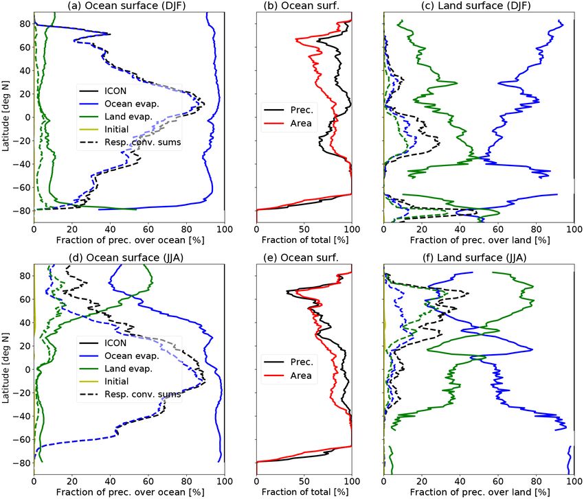
5116                                                     J. Eckstein et al.: Simulating water isotopologues with ICON-ART-Iso

tio α depends on temperature and is different over water and         2.4     Saturation adjustment
over ice (termed αliq and αice ). The parameterizations by Ma-
joube (1971) and by Horita and Wesolowski (1994) have                Cloud water is formed by saturation adjustment in ICON.
been implemented for αliq and those by Merlivat and Nief             Vapor in excess of saturation vapor pressure is transferred
(1967) for αice . Note the definition for α given in Eq. (2) is      to cloud water and temperature is adjusted accordingly. This
also used in COSMOiso (Pfahl et al., 2012) and is the inverse        is repeated in an iterative procedure. For the isotopologues,
of the definition used by others, e.g., by Blossey et al. (2010).    the iteration does not have to be repeated. Instead, Eq. (5)
                                                                     is applied directly using the adjusted values of ICON water.
2.3     Surface evaporation                                          This is the same equation used in COSMOiso (Pfahl et al.,
                                                                     2012) and by Blossey et al. (2010).
Surface evaporation is the source for the atmospheric wa-
ter cycle. In ICON-ART-Iso, the evaporative surface flux is                   hq + hq
                                                                     h          v      c
split into evaporation from land and water surfaces, transpi-         qc =            lq
                                                                                                                                   (5)
                                                                             1 + αliq lqv
ration from plants, and dew and rime formation. Transpira-                               c

tion is considered a non-fractionating process (Eq. 1), which
                                                                     2.5     Microphysics
is an assumption also made by Werner et al. (2011) and Pfahl
et al. (2012). Dew and rime formation (and condensation on           Several grid-scale microphysical schemes are available
the ocean surface) are considered to fractionate according to        in ICON. ICON-ART-Iso makes use of the two-moment
equilibrium fractionation (Eq. 2). For the evaporation part of       scheme by Seifert and Beheng (2006). This scheme com-
the full surface flux, two parameterizations have been imple-        putes the mass and number densities of vapor, cloud wa-
mented (Pfahl and Wernli, 2009; Merlivat and Jouzel, 1979).          ter, rain and four ice classes (ice, snow, graupel and hail)
Both build on the Craig–Gordon model (Craig and Gordon,              and can be used to simulate aerosol–cloud interaction; see
1965; Gat, 2010). Equation (3) gives the general expression          Rieger et al. (2017). As the isotopologues are diagnostic val-
for Revap .                                                          ues, the number densities do not have to be simulated sepa-
               αliq Rsurf − hRv                                      rately. The two-moment scheme describes more than 60 dif-
Revap = k ·                                                   (3)    ferent processes, but only those processes that include the
                     1−h                                             vapor phase lead to fractionation. All others are described by
Here, h is the specific humidity of the lowest model layer           Eq. (1) in the model. Isotopic effects also occur during freez-
relative to the specific humidity at the surface and k is the        ing of the liquid phase (Souchez and Jouzel, 1984; Souchez
nonequilibrium fractionation factor. The two parameteriza-           et al., 2000), but this is neglected due to the low diffusivities,
tions differ in their description of k. While Merlivat and           as in COSMOiso. In accordance with Blossey et al. (2010)
Jouzel (1979) give a parameterization that depends on the            and Pfahl et al. (2012), sublimation is also assumed not to
surface wind, Pfahl and Wernli (2009) have simplified this to        fractionate. Condensation to form liquid water happens only
be wind speed independent. In summary, Eq. (4) is used to            during the formation of cloud water and is accounted for by
calculate the surface flux of the isotopologues, hF tot .            the saturation adjustment. The fractionating processes that
                                                                     remain are ice formation by nucleation, vapor deposition (on
h tot
F       = lF evap · Revap + lF transp · Rsurf + lF dew               all four ice classes) and evaporation of liquid hydrometeors.
            Rv l rime Rv                                             Besides rain, a fraction of the three larger ice classes (snow,
          ·      +F       ·                                   (4)    graupel, hail) can evaporate after melting. This liquid water
            αliq            αice
                                                                     fraction is currently not a prognostic variable.
   For transpiration and evaporation, the isotopologue ratio of         The two-moment scheme by Seifert and Beheng (2006)
the surface water and groundwater (Rsurf ) is necessary. The         uses mass densities instead of mass ratios, so we adopt the
surface model TERRA (included in ICON) was not extended              change in notation here, denoting mass densities by ρ. Vapor
with isotopologues, so Rsurf is not available as a prognostic        pressures are denoted by e. The star (∗ ) indicates values at
variable. Over land, it is therefore approximated by RVSMOW          saturation with respect to liquid (index l) or ice (index i).
in Eqs. (3) and (4). Of course, this is a simplification that           For evaporation of rain and melting hydrometeors, the
allows for the testing of the atmospheric physics package            semiempirical parameterization of Stewart (1975) has been
and will be developed further. Over the ocean, the dataset           implemented and is discussed in this paper. It allows for the
provided by LeGrande and Schmidt (2006) has been imple-              exchange of heavy isotopologues with the surroundings in
mented. Values for HDO are given in this dataset, while those        supersaturated as well as subsaturated conditions. The corre-
for H18
      2 O are determined from the relationship given by the
                                                                     sponding transfer rate is given in Eq. (6). The equation is
global meteoritic water line (GMWL), δD = 8 δ 18 O + 10 ‰            given in the formulation for the evaporation of rain, with
(Craig, 1961).                                                       details on the evaporation of melting ice hydrometeors ex-
                                                                     plained below. In this process, it is assumed that the isotopic
                                                                     content within each droplet is well mixed, which is a simpli-

Geosci. Model Dev., 11, 5113–5133, 2018                                                      www.geosci-model-dev.net/11/5113/2018/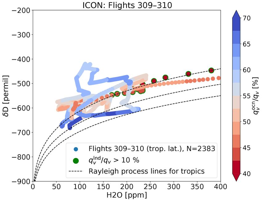
J. Eckstein et al.: Simulating water isotopologues with ICON-ART-Iso                                                           5117

fication when compared to, e.g., Lee and Fung (2008).
               h n h                                             h ice
h evap           D         l ∗      h
                                         i                          Sx     = αk Rvl Sxice                                        (9)
 Sr      =A     lD
                      R  α   ρ
                        r liq l,∞ −  ρ v                    (6)
                                                                                         (1 + Bi ) lSi
                                                                   αk =                                                         (10)
     4π a lf lD                                                               lf lD
                                                                                      lS − 1       + αice 1 + Bi lSi
A=                                                          (7)             hf hD       i
      1 + Bl                                                               lD L2 le∗
     lD L2 le∗                                                               v s i,∞
           e l,∞                                                   Bi =                                                         (11)
Bl =                                                        (8)             ka R2v T∞
                                                                                    3
      ka R2v T∞3

                                                                   2.6     Convection
Here, a is the radius of the hydrometeor, lf is the ventilation
factor, Rv and Rr are the isotopologue ratios in the vapor and     ICON uses the Tiedtke–Bechtold scheme for simulating con-
the hydrometeor, Rv is the gas constant of water vapor, and        vective processes (Tiedtke, 1989; Bechtold et al., 2014). The
Le and ka are the latent heat of evaporation and the heat con-     scheme uses a simple cloud model considering a liquid frac-
ductivity in air. The index ∞ indicates that values are evalu-     tion in cloud water (denoted here by ω) and the remaining
ated for the surroundings. The ratio of the diffusion constants    solid fraction (1ω). Fractionation happens during convective
D is given by the literature values cited above and can be         saturation adjustment (during initialization of convection and
chosen at the time of simulation for each isotopologue. The        in updrafts), in saturated downdrafts and in evaporation be-
tuning parameter n is set to 0.58 by default (Stewart, 1975),      low cloud base. The parameterizations are the same as those
but can be changed at runtime.                                     implemented by Pfahl et al. (2012) in COSMOiso.
    Note that an alternative parameterization to describe the         Convective saturation adjustment calculates equilibration
fractionation of evaporating or equilibrating hydrometeors         between vapor and the total condensed water (liquid and ice).
(that of Blossey et al., 2010) has also been implemented in        The parameterization used for grid-scale adjustment there-
the model. For completeness, the physics of this parameter-        fore has to be expanded in order to be used in convection
ization are briefly explained in Appendix B in comparison          if the liquid water fraction is smaller than one. The isotopo-
to Stewart (1975). An investigation of this parameterization       logue ratio is determined over liquid and ice particles sepa-
and the difference to Stewart (1975) will be provided in a         rately. A closed system approach (Gat, 1996) is used for the
later study.                                                                          by liq
                                                                   liquid fraction (Rv       of Eq. 12). The underlying assumption
    The underlying equation for both parameterizations is de-      for Eq. (13) used for the ice fraction is a Rayleigh process
rived from the fundamentals of cloud microphysics (see             with the kinetic fractionation factor αeff following Jouzel and
Pruppacher and Klett, 2012). It is also used in the microphys-     Merlivat (1984). The two are then recombined according to
                                      evap
ical scheme of ICON, in which lSx = A(lρl,∞      ∗ − lρ ). The
                                                         v         the fraction of liquid water, following Eq. (14). This proce-
definitions of a and lfv depend on whether Sx is calculated        dure has been adopted from COSMOiso (Pfahl et al., 2012).
for rain (Seifert, 2008) or melting ice class hydrometeors
                                                                     by liq                         αliq
(Seifert and Beheng, 2006). For melting ice class hydrome-         Rv         = Rvold          lq new
                                                                                                                                (12)
                                                                                                  v
teors, the melting temperature of ice (T0 = 273.15 K) is used                     1+       (αliq − 1)
                                                                                                lq old
                                                                                                  v
for the calculation of αliq and in place of T∞ . This implies an                   l new αeff −1
additional factor of T∞ /T0 for melting ice hydrometeors, as        by ice           q
le∗
                                                                   Rv      = Rvold l vold                                       (13)
  l,∞ is always evaluated at T∞ . Equation (6) otherwise also
                                                                                     qv
holds true for the evaporation of melting ice hydrometeors.        Rv = (1 − ω) · Rv
                                                                                            by ice          by liq
                                                                                                     + ω · Rv                   (14)
    Fractionation during the nucleation of ice particles or de-
position on one of the four ice class hydrometeors is param-       Here, the indices “old” and “new” denote the values of the
eterized following Blossey et al. (2010), as in COSMOiso           respective variables before and after the convective satura-
(Pfahl et al., 2012). The flux is assumed to interact only with    tion adjustment. The factor αeff , which appears in Eq. (13),
the outermost layer of the hydrometeor, the isotopologue ra-       is determined by Eq. (15). The supersaturation with respect
tio of which is set to be identical to that of the depositional    to ice, ξice , is calculated from Eq. (16), where T0 = 273.15 K
flux. The transfer rate hSxice is then given by Eq. (9) with the   is used. The tuning parameter λ is set to 0.004 in the standard
fractionation factor αk as given in Eq. (10). All symbols are      setup, following Pfahl et al. (2012) and Risi et al. (2010).
used as above, with Ls being the latent heat of sublimation.
                                                                                ξice ζ
                                                                   αeff =                                                       (15)
                                                                          ξice − 1 + αice ζ
                                                                   ξice = 1 − λ(T − T0 )                                        (16)

                                                                     Convective downdrafts are assumed to remain saturated
                                                                   by continuously evaporating precipitation (Tiedtke, 1989). In

www.geosci-model-dev.net/11/5113/2018/                                                       Geosci. Model Dev., 11, 5113–5133, 2018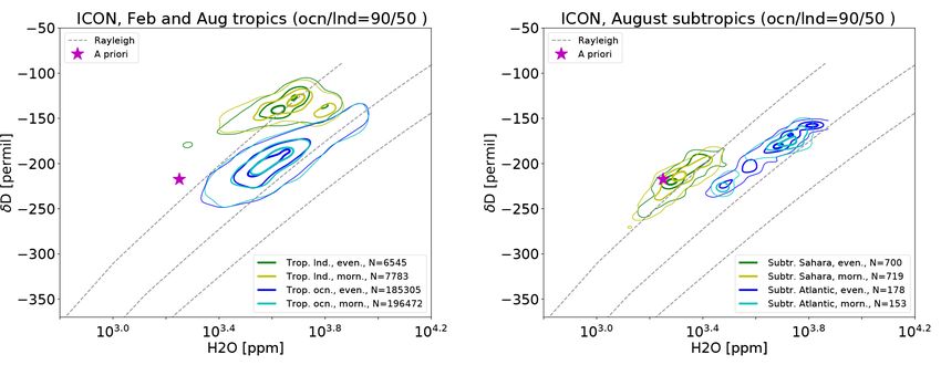
5118                                                   J. Eckstein et al.: Simulating water isotopologues with ICON-ART-Iso

these saturated downdrafts, equilibrium fractionation is ap-        Table 1. Values for the initialization with mean measured δ values.
plied for the liquid fraction, while the ice fraction is assumed    The literature provides the values for HDO, and values for H18 2 O
to sublimate without fractionation.                                 have been determined from GMWL (Craig, 1961).
   Evaporation of precipitation below cloud base is an im-
portant process for several reasons: it leads to a drop in the                        Literature                  HDO        H18
                                                                                                                              2 O
temperature and therefore influences dynamics, but is also              δbottom       Gat (2010)                   −50        −5
important for the isotopic composition (Risi et al., 2008). To          δtropopause   Steinwagner et al. (2007)   −650       −80
describe fractionation here, the parameterization by Stewart            δtop          Steinwagner et al. (2007)   −400     −48.75
(1975) is again applied to the liquid fraction. Different to            δoffset       Gat (2010)                  −100     −11.25
Eq. (6) for evaporation during microphysics, the integrated
form is now applied. Following Stewart (1975), the ratio in
the liquid part of the general hydrometeor after evaporation        taken from Gat (2010). All values are given in Table 1. By
  liq
Radj is given with Eq. (17). Here, f is the fraction of remain-     using the local tropopause height, an adaptation to the local
ing condensate. Rhydold is the isotopologue ratio in the hydrom-    meteorological situation is ensured. To calculate the δ value
eteor before adjustment and RH is the relative humidity cal-        of the hydrometeors, a constant offset is applied to the local δ
culated as the vapor pressure over saturation vapor pressure.       value of vapor. The literature provides values for HDO, while
                                                                  those for H18
                                                                               2 O are determined from the relationship given by
  liq                   old
Radj = γ Rv + f β Rhyd      − γ Rv                           (17)   the global meteoritic water line (GMWL; Craig, 1961).
      RH
γ=                                                          (18)
   αliq − µ                                                         3   Model evaluation results
   αliq − µ
β=                                                          (19)    In the following sections, we present the first results and
       µ
             h −n                                                 comparisons of model simulations with measurements span-
               D                                                    ning several spatiotemporal scales: Sect. 3.1 shows how the
µ = (1 − RH) l                                              (20)
               D                                                    model-simulated diagnostic H2 O can be used to investigate
                                                                    source regions of the (modeled) water cycle. Section 3.2
Using Eq. (17), the isotopologue ratio in the adjusted hy-          compares results for precipitation from the same long model
drometeor is given with Eq. (21). The ice fraction is assumed       integration with measurements taken from the GNIP network
to sublimate without fractionation, maintaining its isotopo-        (Terzer et al., 2013; IAEA/WMO, 2017). Section 3.3 looks at
logue ratio.                                                        seasonal and regional differences by comparing model out-
               old         liq                                      put with pairs of {H2 O, δD} derived from IASI satellite mea-
Radj = (1 − ω)Rhyd + ωRadj                                  (21)    surements (Schneider et al., 2016). Finally, Sect. 3.4 presents
                                                                    a first case study, in which simulated values of δD are
Following Pfahl et al. (2012), an additional equilibration has
                                                                    compared with measurements from the IAGOS-CARIBIC
been implemented to determine the final isotopologue ratio
                                                                    project (Brenninkmeijer et al., 2007). All simulations dis-
of the hydrometeors, which is given in Eq. (22). The parame-
                                                                    cussed here are free-running.
ter ξadd is a tuning parameter that is set to 0.5 in the standard
                                                                       In the following sections, we focus on H2 O (ICON stan-
setup.
                                                                    dard water), HDO and H18   2 O. The settings for each isotopo-

                           Rv
                                                                   logue are defined at runtime, which is why the specifications
  final
Radj = Radj + ξadd · ω          − Radj                       (22)   for the simulations are given here. The diffusion constant
                           αliq
                                                                    ratio is set to the values of Merlivat and Jouzel (1979) and
2.7    Initialization of the isotopologues                          the equilibrium fractionation is parameterized following Ma-
                                                                    joube (1971) over liquid water and following Merlivat and
A meaningful initialization is an important prerequisite for        Nief (1967) over ice. Surface evaporation is described by the
any simulation, also of the isotopologues. In addition to an        parameterization of Pfahl and Wernli (2009). The parameter-
initialization with a constant ratio to standard water, the iso-    ization by Merlivat and Jouzel (1979) has little influence on
topologues can be initialized with the help of mean measured        the values in the free troposphere and is not discussed further.
δ values. Values at the lowest model level, the tropopause          The dataset by LeGrande and Schmidt (2006) for the isotopic
level (WMO definition; see Holton et al., 1995) and the             content of the ocean surface is used for all isotopologues. The
model top are prescribed for vapor, and linear and log-linear       grid-scale evaporation of hydrometeors is described by the
interpolation is applied below and above the tropopause, re-        parameterization by Stewart (1975) if not noted differently.
spectively. Values for the tropopause level and the model top          In addition to ICON standard water, three diagnostic sets
are taken from MIPAS measurements (Steinwagner et al.,              of water tracers are simulated. All fractionation is turned off,
2007), and the value at the lowest level is a standard value        so they resemble H2 O. But the evaporation and initialization

Geosci. Model Dev., 11, 5113–5133, 2018                                                www.geosci-model-dev.net/11/5113/2018/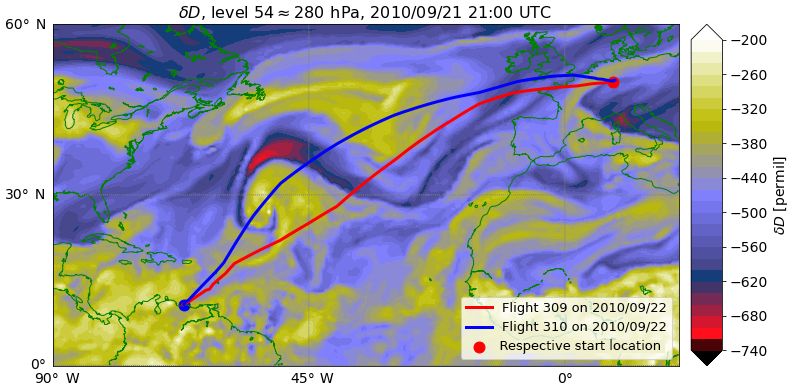
J. Eckstein et al.: Simulating water isotopologues with ICON-ART-Iso                                                            5119

are different: water indexed by init (as in q init ) is set to        area fraction largely determines the overall fraction of rain
ICON water at initialization, but evaporation is turned off. In       that falls over the ocean or over land. This is why the other
the course of the simulation, water of this type precipitates         panels display values of P relative to the sum over each com-
out of the model atmosphere. Water indexed by ocn and                 partment, not to the total sum.
lnd is initialized with zero and evaporates from the ocean               To evaluate the model simulation, we use values starting
(q ocn ) and land areas (q lnd ), respectively. The sum of q init ,   in the second year. At this time, the tropospheric moisture
q ocn and q lnd always equals the mass mixing ratio of ICON           has been completely replaced by water that has evaporated
standard water, indexed as q ICON . These tracers allow us to         during the model run. This is demonstrated by the values of
infer the relative importance of ocean and land evaporation           P init close to zero in all panels in Fig. 1. Technically, this
– essentially the source of water in the model atmosphere –           means that the ternary solution of q init , q ocn and q lnd that
at all times. In addition to case studies, this is interesting be-    makes up q ICON is practically reduced to a binary solution
cause of the simplified implementation of isotopic processes          of only q ocn and q lnd . Other experiments show that this is
during land evaporation in the current version of ICON-ART-           already true after a few weeks (not shown).
Iso; see Sect. 2.3. The tracers of q init provide information on         During Northern Hemisphere winter over the ocean
the importance of the initialization at a certain time in the         (Fig. 1a), the precipitation is strongly dominated by water
simulation.                                                           that has evaporated from the ocean. Water from the land sur-
                                                                      face hardly reaches the ocean. Over land areas, the ocean
3.1   An application of diagnostic water tracers:                     is also the dominant source for precipitation, reaching more
      precipitation source regions                                    than 50 % at almost all latitudes. In the Northern Hemisphere
                                                                      midlatitude land areas, more than 70 % of the precipitated
This section examines the moisture source regions of pre-             water originates from the ocean. The tropical and Southern
cipitation over ocean and land. Gimeno et al. (2012) give a           Hemisphere land areas (in DJF) receive up to 40 % of precip-
review of the subject, while, e.g., Numaguti (1999), Van der          itation from land evaporation. Most precipitation at tropical
Ent et al. (2010) and Risi et al. (2013) study this question by       and subtropical latitudes over the ocean originates from con-
use of other models and in more detail.                               vection (indicated by dashed lines). The role of convection is
   Here, we use a decadal model integration. The simulation           much smaller over land areas and again stronger in the South-
was initialized with ECMWF (European Centre for Medium-               ern Hemisphere. Note that in a simulation with very high hor-
Range Weather Forecasts) Integrated Forecast System (IFS)             izontal resolution (for an example using ICON; see Klocke
operational analysis data on 1 January 2007, 00:00 UTC, to            et al., 2017), more convective processes could have been di-
simulate 11 years on an R2B04 grid (≈ 160 km horizontal               rectly resolved. In this specific case of a resolution close to
resolution). The time step was set to 240 s (convection called        160 km, practically no convection is directly resolved by the
every second step) and output was saved on a regular 1◦ × 1◦          model. It should therefore be considered that the amount of
grid every 10 h in order to obtain values from all times of the       precipitation from convection only shows the importance of
day. Sea surface temperatures and sea ice cover were updated          this parameterization in the simulations at this resolution.
daily by linearly interpolating monthly data provided by the             The distribution of precipitation water sources is differ-
AMIP II project (Taylor et al., 2000). The first year is not          ent in Northern Hemisphere summer (bottom row of Fig. 1).
considered as spin-up time of the model and the simulation            In summer, the Northern Hemisphere land areas (bottom
is evaluated up to the end of 2017.                                   right) supply themselves with a substantial fraction of the
   We look at the total precipitation P in Northern Hemi-             moisture that then precipitates. The importance of convec-
sphere winter (December, January, February, denoted by                tion is increased in Northern Hemisphere summer with its
DJF) and summer (June, July, August, denoted by JJA). Fig-            maximum influence shifted into northern midlatitudes. De-
ure 1 displays zonal sums of P init , P ocn and P lnd relative to     spite the larger moisture availability over the ocean, the far
standard water precipitation P ICON as a function of latitude.        Northern Hemisphere land areas also supply the larger part
The sum of precipitation that originates from convection is           of moisture that precipitates over the ocean in summer; see
also given for each water species. The top panels give winter         Fig. 1d.
values, while the bottom panels display the results for sum-             These results are comparable to the studies by Numaguti
mer months.                                                           (1999), Van der Ent et al. (2010) and Risi et al. (2013). While
   The area covered by ocean is not equally distributed over          these studies look at regional differences, the latitudinal de-
different latitudinal bands, which is the reason why ocean            pendence is similar to the results presented here. This first
and land points are considered separately. Panels (b) and (e)         application of ICON-ART-Iso – while no isotopologues are
show the fraction of precipitation that has fallen over the           used – shows how diagnostic moisture tracers can be applied
ocean relative to the total precipitation and the area fraction       to better understand specific aspects of the atmospheric water
of the ocean in each latitudinal band. Despite the character-         cycle.
istics of the different seasons, which will be discussed in the
following paragraphs, the latitudinal distribution of the ocean

www.geosci-model-dev.net/11/5113/2018/                                                  Geosci. Model Dev., 11, 5113–5133, 2018
5120 J. Eckstein et al.: Simulating water isotopologues with ICON-ART-Iso
Figure 1. Fractional contributions of P ICON , P init , P ocn and P lnd to zonal sums of total precipitation for Northern Hemisphere winter
(DJF, a–c) and summer (JJA, d–f) as a function of latitude. Outer panels show sums over the ocean and land grid points, respectively. Here,
dashed lines indicate the contribution of convective precipitation for each source of atmospheric water. Center panels display the fraction of
precipitation over the ocean relative to total precipitation (over land plus ocean) and the fraction of the area covered by ocean.
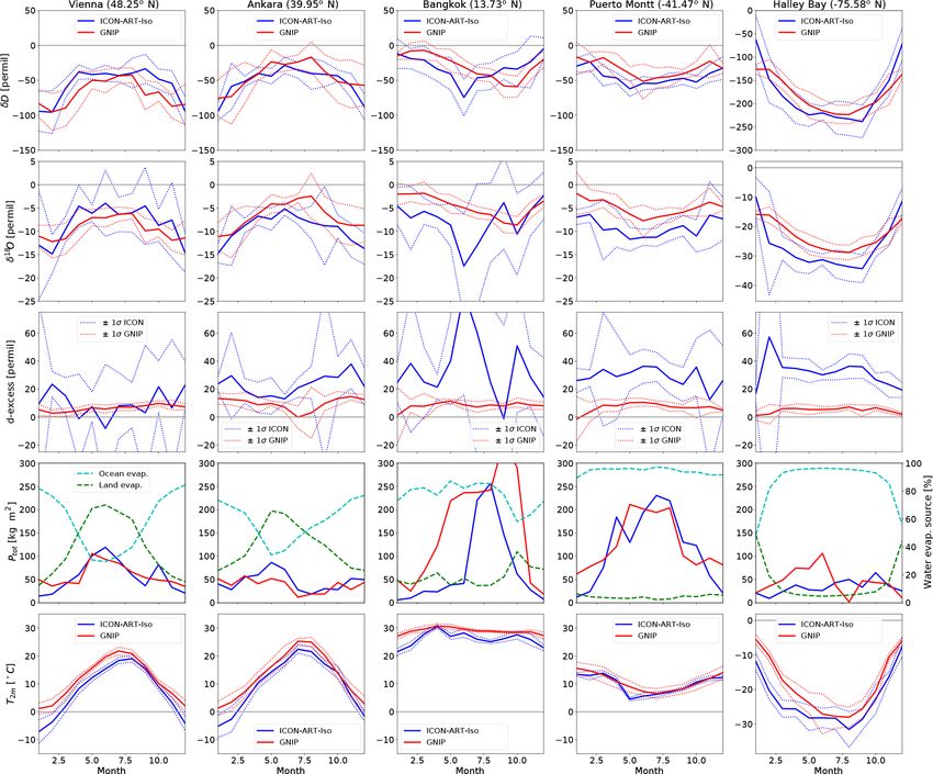
3.2 The multi-annual simulation compared to GNIP culated for δD, δ 18 O and d-excess (d-excess = δD − 8 δ 18 O)
data in precipitation, total precipitation P and 2 m temperature
T2m . The corresponding values are available from GNIP. Re-
For a first validation of δD and δ 18 O values, we use the sults are displayed in Fig. 2. The panels for total precipitation
decadal ICON-ART-Iso model integration of the previous also include the fractional contribution to precipitation by
section and compare results to data taken from the GNIP ocean and land evaporation (see previous section). All panels
network (Global Network for Isotopes in Precipitation; see (except for the precipitation amount) show the 1σ standard
Terzer et al., 2013; IAEA/WMO, 2017). In this section, we deviation range for model and measurement data.
analyze δ values in total precipitation. For most stations, the seasonal cycle of precipitation is
Five GNIP stations were chosen for their good data avail- reproduced by the model. This includes the summer mini-
ability in the respective years, sampling different climate mum for Ankara and the strong winter precipitation in Puerto
zones: Vienna in eastern Austria (48.2◦ N, 16.3◦ E) in cen- Montt. Precipitation is underestimated for Bangkok, espe-
tral Europe, Ankara in central Anatolia (40.0◦ N, 32.9◦ E), cially in Northern Hemisphere spring. For all stations, the
Bangkok in tropical southern Asia (13.7◦ N, 100.5◦ E), influence of land evaporation is strongest in their respective
Puerto Montt in central Chile (41.5◦ S, 72.9◦ W) and Hal- summer. Vienna and Ankara show a decreasing influence of
ley station in Antarctica (75.6◦ S, 20.6◦ W). The closest grid the ocean in winter, typical for a more continental climate.
point to each of these stations was taken from the model out- For Puerto Montt, located between the Pacific and the An-
put and the multiyear mean of each calendar month was cal-
Geosci. Model Dev., 11, 5113–5133, 2018 www.geosci-model-dev.net/11/5113/2018/J. Eckstein et al.: Simulating water isotopologues with ICON-ART-Iso 5121
Figure 2. Monthly mean data for five GNIP stations (left to right: Vienna, Ankara, Bangkok, Puerto Montt and Halley station). Variables
listed from top to bottom: δD, δ 18 O, d-excess (δD − 8 δ 18 O), total precipitation Ptot and 2 m temperature (T2m ). Plots showing Ptot also
include the percentage of land and ocean evaporation in precipitation. The 1σ standard deviation interval is indicated by dashed lines (except
P for readability).
dean mountain range, and for Bangkok, almost all precipitat- as the Southern Hemisphere. Values of d-excess are also of
ing water originates from the ocean. similar magnitude. Model data are more variable than the
The seasonal cycle of temperature is reproduced for all sta- measurements. However, the model data are mostly within
tions. Winter temperatures are too cold in this model config- the standard deviation range of measurements. This demon-
uration for all stations. This temperature bias can partly be strates the capability of ICON-ART-Iso to simulate climato-
explained by the fact that the altitude of all stations is higher logical patterns. The seasonal cycle and regional differences
in the model because of the coarse grid, e.g., 550 m for the in δD and δ 18 O are correctly reproduced in this climatologi-
grid point identified with Vienna versus 198 m for the GNIP cal integration.
station. Also, the measured temperatures are slightly higher
than mean monthly ERA-Interim (Dee et al., 2011) 2 m tem- 3.3 Comparison with IASI satellite data for a seasonal
peratures for the corresponding grid points (not shown). perspective
Despite some biases, the mean values of δD and δ 18 O are
well reproduced by ICON-ART-Iso for all five stations. The Here, we compare pairs of {H2 O, δD} retrieved from
seasonal cycle is captured correctly in the Northern as well MetOp/IASI remote sensing measurements with data from
www.geosci-model-dev.net/11/5113/2018/ Geosci. Model Dev., 11, 5113–5133, 20185122 J. Eckstein et al.: Simulating water isotopologues with ICON-ART-Iso
two simulations. The section closely follows the case stud- in Sect. 3.1, the amount of water remaining in the tropo-
ies presented by Schneider et al. (2017), who compared sphere from initialization is negligible by using lead times
IASI retrievals and data from the global hydrostatic model of 3 months. For this study, model output was interpolated
ECHAM5-wiso (Werner et al., 2011). to a regular 0.36◦ × 0.36◦ grid, which is close to the 40 km
resolution of the numerical ICON grid in the tropics. Output
3.3.1 IASI satellite data and model post-processing was written for every hour of simulation.
IASI observations are only available at cloud-free condi-
IASI (Infrared Atmospheric Sounding Interferometer) A and tions. In order to exclude cloud-affected grid points in the
B are instruments onboard the MetOp-A and MetOp-B satel- ICON data, the total cloud cover simulated by ICON was
lites (Schneider et al., 2016). They measure thermal in- used, denoted by Cclct . All points with Cclct > 90 % were
frared spectra in nadir view from which free-tropospheric excluded. The parameter Cclct goes into saturation quickly
{H2 O, δD} pair data are derived. As the satellites circle the and 90 % is reached even for thin clouds. Surface emissivity
earth in polar sun-synchronous orbit, each IASI instrument Esrf is a necessary input parameter for the retrieval simula-
takes measurements twice a day at local morning (approxi- tor. In this first study, Esrf was set to 0.96 over land and 0.975
mately 09:30) and evening (approximately 21:30). The mea- over the ocean. This is in accordance with the mean values as
surements are most sensitive at a height of approximately given by Seemann et al. (2008). In addition, Schneider et al.
4.9 km. An IASI {H2 O, δD} pair retrieval method has been (2017) show in a sensitivity study that errors on the order of
developed and validated in the framework of the project MU- 10 % in this value have only a limited influence on the av-
SICA (MUlti-platform remote Sensing of Isotopologues for eraging kernels as simulated by the retrieval simulator. We
investigating the Cycle of Atmospheric water). The MU- follow the method outlined by Schneider et al. (2017) and
SICA retrieval method is presented by Schneider and Hase use values only when the sensitivity metric serr < 0.05.
(2011) and Wiegele et al. (2014) with updates given in We examine results for different areas over ocean and over
Schneider et al. (2016). land using all data from the satellite and the model in the
Schneider et al. (2017) present guidelines for comparing respective areas. The scatter of {H2 O, δD} is not shown di-
model data to the remote sensing data. First, retrieval simu- rectly. Instead, the figures show the isolines of relative nor-
lator software is used for simulating the MUSICA averaging malized frequency, which is explained in Appendix A. In ad-
kernel using the atmospheric state of the model atmosphere. dition, Rayleigh fractionation curves are indicated in all fig-
The simulated kernel is then applied to the original model ures. These are the same as those given by Schneider et al.
state (x) in order to calculate the state that would be reported (2017).
by the satellite retrieval product (x̂, see Eq. 23).
3.3.2 Seasonal and daily cycle
x̂ = A(x − x a ) + x a (23)
Here, A is the simulated averaging kernel and x a the a pri- Seasonal and daily cycle are investigated in {H2 O, δD} space.
ori state. The a priori value used in the retrieval process for The seasonal cycle is discussed for different regions over the
4.9 km is at {1780 ppm, −217.4 ‰}. This value represents the central Pacific Ocean. The daily cycle is considered in the
climatological state of the atmosphere. In the retrieval pro- tropics and subtropics, also investigating differences between
cess, the satellite radiance measurements are used for esti- land and ocean areas.
mating the deviation of the actual atmospheric state from the First, the seasonal cycle over the Pacific Ocean is exam-
a priori assumed state, and it is important to note that the re- ined by comparing the two target periods in different ar-
mote sensing retrieval product is not independent from the eas (140◦ E < λ < 220◦ E longitude and different latitudinal
a priori assumptions (see Schneider et al., 2016, for more bins). Results are presented in Fig. 3, which includes the ex-
details). In Schneider et al. (2017), these guidelines have act latitudes. IASI data (bottom panels) show the specific
been followed for comparison of IASI data with ECHAM5- characteristics of the different regions. H2 O content is high-
wiso model data. We use the same approach for comparisons est for tropical air masses and lowest for the highest latitudes
to ICON-ART-Iso and our results can be directly compared in February and August. At the same time, tropical air is least
to the results from the hydrostatic global model ECHAM5- depleted in HDO, while the highest latitudes show the low-
wiso. est values of δD, i.e., are more depleted. When comparing
In order to compare ICON-ART-Iso measurements with February and August values at each latitude, a clear seasonal
IASI data, a simulation of 12 months is used, which was signal appears everywhere except for the tropics: during sum-
initialized on 5 November 2013. This simulation uses a mer of the corresponding hemisphere, the air is more humid
finer resolution of R2B06, corresponding to roughly 40 km. and more depleted in HDO. The distributions seem to shift
Again, we use varying ocean surface temperatures and sea from season to season along a line perpendicular to those of
ice cover; see the specifications in Sect. 3.1. As in Schneider the Rayleigh model. The distribution in the tropics shows a
et al. (2017), two target time periods are investigated from broadened shape in August.
12–18 February and 12–18 August. As has been pointed out
Geosci. Model Dev., 11, 5113–5133, 2018 www.geosci-model-dev.net/11/5113/2018/J. Eckstein et al.: Simulating water isotopologues with ICON-ART-Iso 5123 Figure 3. Isolines of the relative normalized frequency distribution for pairs of δD and H2 O (see Appendix A for the method) after processing ICON-ART-Iso data with the IASI retrieval simulator of Schneider et al. (2017) (a, b) and IASI data for the same time (c, d). Data from morning overpasses are shown for 12 to 18 February (a, c) and 12 to 18 August (b, d) 2014 for different latitudinal bands over the Pacific Ocean (140◦ E < λ < 220◦ E longitude). Contour lines are indicated at 0.2, 0.6 and 0.9 of the normalized distribution. The results of ICON-ART-Iso are shown in the top pan- most identical. Over land, the water vapor in the tropics and els of Fig. 3. The latitudinal dependence is similar to IASI: subtropics is more depleted of HDO in the morning. There is high H2 O and δD in the tropics and lower values for midlat- also a daily cycle in H2 O in the tropics: during morning over- itudes. The range of values is also very similar. The seasonal passes, H2 O values are higher than in the evening. Schneider cycle in H2 O and δD is also reproduced to some degree, es- et al. (2017) argue that this is due to the cloud filter, which re- pecially in the subtropical latitudes. The most obvious dif- moves areas of heavy convection in the evening. In the morn- ferences to IASI results occur in the Northern Hemisphere ing, the clouds have disappeared, but high humidity remains, midlatitudes in summer, which show less negative values of especially in the lower troposphere. This may partly be due δD in the model than in the satellite data, especially for hu- to evaporation of raindrops, which explains the enhanced de- mid situations. In winter, this may also be the case, but there pletion in HDO (Worden et al., 2007). Over the Sahara (the are only a few humid values simulated at all or available in subtropical land area considered), the daily cycle is different: the satellite dataset. In general, the model shows a similar be- while mixing ratios of H2 O rise only slightly during the day, havior as ECHAM5-wiso, the results of which are presented there is a strong increase in the HDO content in the evening. by Schneider et al. (2017). This behavior can be attributed to vertical mixing (Schneider For the daily cycle in the tropics and subtropics, land and et al., 2017, and references therein). ocean points are considered separately (Fig. 4; see caption The data retrieved from ICON-ART-Iso model simulations for exact definition of the bins). IASI shows a clear signal are shown in the top panels of Fig. 4. Tropical air (panel a) of the daily cycle for both the tropics and subtropics over over the land shows slightly lower mixing ratios for H2 O than land (bottom panels of Fig. 4). There is no such signal over IASI. The humidity of tropical ocean points is better repro- the ocean, where morning and evening distributions are al- duced. The difference in δD is stronger for both areas, with www.geosci-model-dev.net/11/5113/2018/ Geosci. Model Dev., 11, 5113–5133, 2018
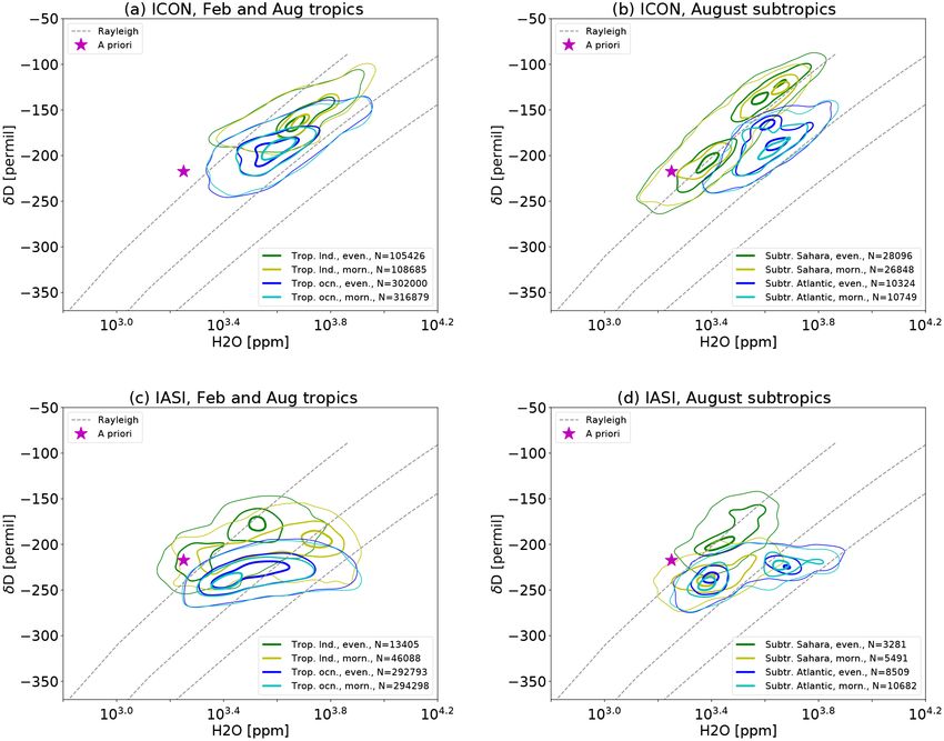
5124                                                     J. Eckstein et al.: Simulating water isotopologues with ICON-ART-Iso

Figure 4. Isolines of the relative normalized frequency distribution for pairs of δD and H2 O (see Appendix A for the method) after processing
ICON-ART-Iso data with the IASI retrieval simulator of Schneider et al. (2017) (a, b) and IASI data for the same time (c, d). (a, c) Data
corresponding to morning and evening overpasses for the tropics (10◦ S < ϕ < 10◦ N, all longitudes, summer and winter simulation) over
land and over the ocean. (b, d) Morning and evening overpasses for the subtropics (22.5◦ S < ϕ < 35◦ N, summer simulation) over land
(Saharan desert region, 10◦ W < ϕ < 50◦ E) and Atlantic Ocean (50◦ W < ϕ < 30◦ W). Contour lines are indicated at 0.2, 0.6 and 0.9 of the
normalized distribution.

δD values being too high in the model. There is no daily cy-             humidity tracers q ocn and q lnd . As has been pointed out in
cle in the tropics for ICON-ART-Iso. The subtropical mix-                Sect. 3.1, q init is negligible 3 months after initialization. To
ing ratios (panel b) of H2 O over the ocean are similar to               distinguish between grid points mostly influenced by ocean
those in the tropics but cover a smaller range than those re-            or land evaporation, we additionally use the following cri-
trieved from IASI. The very humid and very dry parts of the              teria to define ocean and land points: q ocn /q ICON > 0.9 for
IASI distribution are not reproduced by the model. δD val-               grid points over the ocean and q lnd /q ICON > 0.5 for land grid
ues in ICON-ART-Iso are larger than in the IASI retrievals.              points predominantly affected by land evaporation. This in-
As pointed out by Schneider et al. (2017), the daily cycle in            vestigation serves to showcase how the ocean and land evap-
IASI also manifests itself in the number of samples passing              oration tracers can be used and the threshold values are there-
the IASI cloud filter and quality control. The IASI cloud filter         fore arbitrary to some degree. The tracer fields of water evap-
removes much more evening observations than morning ob-                  orating from ocean and land have not been processed with the
servations, meaning more cloud coverage in the evening than              retrieval simulator, and instead values interpolated to 4.9 km
in the morning. In contrast, the ICON-ART-Iso cloud filter               are directly used.
removes a similar amount of data for morning and evening;                   The result is shown in Fig. 5 for the tropics and subtrop-
i.e., in the model morning and evening cloud coverage is                 ics using the same method as for Fig. 4. The characteristics
rather similar. This may also influence the results.                     of the different regions show up much more clearly with the
   To further analyze the influence of ocean and land areas,             additional criteria. For the tropical ocean, the distribution of
the analysis of the daily cycle is repeated, making use of the           H2 O is similar, but the values are slightly more depleted in

Geosci. Model Dev., 11, 5113–5133, 2018                                                      www.geosci-model-dev.net/11/5113/2018/
J. Eckstein et al.: Simulating water isotopologues with ICON-ART-Iso                                                                5125

Figure 5. As Fig. 4 for ICON-ART-Iso. In addition to the land–ocean mask, land data must pass the condition qvlnd /qv > 0.5 and ocean data
must pass qvocn /qv > 0.9.

HDO. The distribution of pairs attributed to the land surface          3.4.1   IAGOS-CARIBIC data and model
is reduced to values with relatively high humidity and en-                     post-processing
riched in HDO. The latter might be due to the signal of plant
evapotranspiration, which is considered a non-fractionation
                                                                       In the European research infrastructure IAGOS-CARIBIC,
process.
                                                                       a laboratory equipped with 15 instruments is deployed on-
   In the subtropics, the distributions over land change their
                                                                       board a Lufthansa A340-600 for four intercontinental flights
shape completely and are separated from those over the
                                                                       per month. Measurements of up to 100 trace gases and
ocean. The distribution for the subtropical ocean remains
                                                                       aerosol parameters are taken in situ and in air samples (Bren-
largely unchanged, becoming slightly more elongated with
                                                                       ninkmeijer et al., 2007). δD is measured using the instrument
lower values in δD. For the land surface, the additional cri-
                                                                       ISOWAT (Dyroff et al., 2010). It is a tunable diode-laser
terion strongly reduces the number of values that are con-
                                                                       absorption spectrometer that simultaneously measures HDO
sidered. This implies that over the Saharan desert, air mostly
                                                                       and H2 O at wave numbers near 3765 cm−1 to derive δD in
influenced by land evaporation (50 % or more) is very dry
                                                                       vapor. The instrument is calibrated based on regular measure-
and highly processed (low δD).
                                                                       ments (each 30 min) of a water vapor standard with 500 ppm
   This section shows that ICON-ART-Iso is able to re-
                                                                       H2 O and δD = −109 ‰. The δD offset is derived by con-
produce regional differences and the seasonal cycle of
                                                                       sidering the data of the driest 5 % of the air masses sampled
{H2 O, δD} of vapor in the lower troposphere. The additional
                                                                       during each flight, which is typically 4–8 ppm H2 O. At the
water diagnostics are used to study the behavior of the model
                                                                       flight altitude of 10–12 km, this is without exception lower-
in more detail and will help investigate measured distribu-
                                                                       most stratospheric air (LMS), for which a δD of −600 ‰ is
tions in future studies.
                                                                       assumed (Pollock et al., 1980; Randel et al., 2012). An as-
3.4   Comparing with in situ IAGOS-CARIBIC                             sumed uncertainty of this LMS value of 400 ‰ translates
      measurements                                                     to a relevant uncertainty of 20 ‰ at 100 ppm H2 O. Due to
                                                                       further sources of measurement uncertainty, the data have a
In this section, we present a first case study, in which results       total flight-specific systematic uncertainty up to 100 ‰. The
of ICON-ART-Iso are compared to in situ measurements of                total uncertainty is humidity dependent, decreasing towards
δD taken by the IAGOS-CARIBIC passenger aircraft at 9–                 higher humidity (e.g., 100 ‰ at 80 ppm H2 O versus less than
12 km of altitude. Two flights in September 2010 are con-              20 ‰ at 500 ppm H2 O; see Christner, 2015, for more details).
sidered, which took place a few days after the passage of                 The in situ IAGOS-CARIBIC data are suitable for the
the tropical cyclone Igor over the Atlantic Ocean. The full            analysis of processes on small scales. δD measurements are
dataset of all δD measurements taken by IAGOS-CARIBIC                  available as 1 min means, which translates to a spatial scale
in the tropics is also used as a reference.                            of approximately 15 km. This horizontal resolution is finer
                                                                       than the chosen ICON-ART-Iso configuration (R2B06 corre-
                                                                       sponding to 40 km) and is therefore suitable for a case study
                                                                       validation. Unfortunately, the uncertainty of δD data at hu-
                                                                       midity below approximately 40 ppm H2 O is too high to be
                                                                       used for analysis. Because of the systematic total uncertainty

www.geosci-model-dev.net/11/5113/2018/                                                     Geosci. Model Dev., 11, 5113–5133, 2018
You can also read