Implementation and assessment of a carbonate system model Eco3M-CarbOx v1.1 in a highly dynamic Mediterranean coastal site Bay of Marseille ...
←
→
Page content transcription
If your browser does not render page correctly, please read the page content below

Geosci. Model Dev., 14, 295–321, 2021
https://doi.org/10.5194/gmd-14-295-2021
© Author(s) 2021. This work is distributed under
the Creative Commons Attribution 4.0 License.

Implementation and assessment of a carbonate system model
(Eco3M-CarbOx v1.1) in a highly dynamic Mediterranean
coastal site (Bay of Marseille, France)
Katixa Lajaunie-Salla1 , Frédéric Diaz1 , Cathy Wimart-Rousseau1 , Thibaut Wagener1 , Dominique Lefèvre1 ,
Christophe Yohia2 , Irène Xueref-Remy3 , Brian Nathan3 , Alexandre Armengaud4 , and Christel Pinazo1
1 Aix Marseille Univ., Université de Toulon, CNRS, IRD, MIO, UM 110, 13288, Marseille, France
2 Aix Marseille Univ., CNRS, IRD, OSU Institut Pythéas, 13288, Marseille, France
3 Aix Marseille Univ., Université d’Avignon, CNRS, IRD, IMBE, Marseille, France
4 AtmoSud: Observatoire de la qualité de l’air en région Sud Provence Alpes Côte d’Azur,

le Noilly Paradis, 146 rue Paradis, 13294 Marseille, France

Correspondence: Katixa Lajaunie-Salla (katixa.lajaunie@gmail.com) and Fredéric Diaz (frederic.diaz@univ-amu.fr)

Received: 16 February 2020 – Discussion started: 18 May 2020
Revised: 17 November 2020 – Accepted: 26 November 2020 – Published: 19 January 2021

Abstract. A carbonate chemistry balance module was imple-        bation. When the seawater temperature changes quickly, the
mented into a biogeochemical model of the planktonic food        behavior of the BoM waters alters within a few days from
web. The model, named Eco3M-CarbOx, includes 22 state            a source of CO2 to the atmosphere to a sink into the ocean.
variables that are dispatched into 5 compartments: phyto-        Moreover, the higher the wind speed is, the higher the air–
plankton, heterotrophic bacteria, detrital particulate organic   sea CO2 gas exchange fluxes are. The river intrusions with
matter, labile dissolved organic, and inorganic matter. This     nitrate supplies lead to a decrease in the pCO2 value, favor-
model is applied to and evaluated in the Bay of Marseille        ing the conditions of a sink for atmospheric CO2 into the
(BoM, France), which is a coastal zone impacted by the           BoM. A scenario of high atmospheric concentrations of CO2
urbanized and industrialized Aix–Marseille Metropolis, and       also favors the conditions of a sink for atmospheric CO2 into
subject to significant increases in anthropogenic emissions of   the waters of the BoM. Thus the model results suggest that
CO2 .                                                            external forcings have an important impact on the carbonate
   The model was evaluated over the year 2017, for which in      equilibrium in this coastal area.
situ data of the carbonate system are available in the study
site. The biogeochemical state variables of the model only
change with time, to represent the time evolution of a sea
                                                                 1   Introduction
surface water cell in response to the implemented realistic
forcing conditions. The model correctly simulates the value      Current climate change mostly originates from the car-
ranges and seasonal dynamics of most of the variables of         bon dioxide (CO2 ) increase in the atmosphere at a high
the carbonate system except for the total alkalinity. Several    annual rate (+2.63 ppm from May 2018 to May 2019,
numerical experiments were conducted to test the response        https://www.esrl.noaa.gov/gmd/ccgg/trends/global.html, last
of carbonate system to (i) a seawater temperature increase,      access: September 2019). This atmospheric CO2 increase im-
(ii) wind events, (iii) Rhône River plume intrusions, and        pacts the carbonate chemistry equilibrium of the oceanic wa-
(iv) different levels of atmospheric CO2 contents. This set of   ter column (Allen et al., 2009; Matthews et al., 2009). Oceans
numerical experiments shows that the Eco3M-CarbOx model          are known to act as a sink for anthropogenic CO2 , i.e., 30 %
provides expected responses in the alteration of the marine      of emissions, which leads to a marine acidification (Gruber
carbonate balance regarding each of the considered pertur-       et al., 2019; Orr et al., 2005; Le Quéré et al., 2018).

Published by Copernicus Publications on behalf of the European Geosciences Union.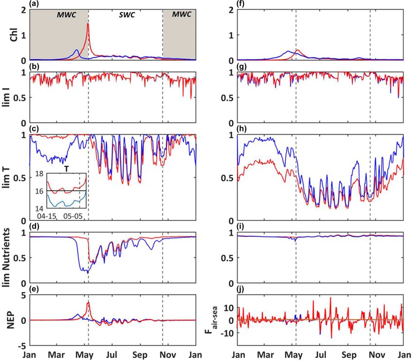
296                                    K. Lajaunie-Salla et al.: A carbonate system model in a Mediterranean coastal site

   CO2 is a key molecule in the biogeochemical function-          ate ions (CO2−3 ) (Hoegh-Guldberg et al., 2018). These trends
ing of the marine ecosystem. Photo-autotrophic organisms,         were already described in several coastal and open-ocean
mainly phytoplankton and macro-algae, fix this gas through        locations worldwide (Cai et al., 2011). In a coastal north-
photosynthesis in the euphotic zone and, in turn, produce         western Mediterranean site, a 10-year time series of in situ
organic matter and dissolved oxygen. Heterotrophic organ-         measurements highlights a trend of pH decrease and pCO2
isms, mainly heterotrophic protists and metazoans, consume        increase (Kapsenberg et al., 2017). Low pH values can in-
organic matter and dissolved oxygen by aerobic respiration        hibit the ability of many marine organisms to form the cal-
and, in turn, produce CO2 . In the ocean, the main processes      cium carbonate (CaCO3 ) used in the making of skeletons
regulating CO2 exchanges between the atmosphere and sea           and shells (Gattuso et al., 2015). In an extreme case, this
are the solubility pump and the biological pump at different      shift may promote dissolution of CaCO3 because the water
timescales. Overall, the thermohaline gradients drive the sol-    will become under-saturated with respect to CaCO3 minerals
ubility pump, while the metabolic processes of gross primary      (Doney et al., 2009).
production and respiration set the intensity of the biological       The present study is dedicated to the implementation of a
pump (Raven and Falkowski, 1999).                                 carbonate system module into a preexisting biogeochemical
   The coastal zones, despite their small surface area and vol-   model of the planktonic food web. This new model, named
ume compared to those of the open ocean, have a large in-         Eco3M-CarbOx (v1.1), is then evaluated in a highly dynamic
fluence upon carbon dynamics and represent 14 % to 30 %           coastal site, i.e., the Bay of Marseille (BoM) in the north-
of the oceanic primary production (Gattuso et al., 1998). At      western Mediterranean Sea. This evaluation is performed
the interface between open ocean and continents, these zones      on the seasonal dynamics of biogeochemical and carbonate
receive large inputs of nutrients and organic matter from         modeled variables against that of the corresponding in situ
rivers, groundwater discharge, and from atmospheric depo-         data available over the year 2017. This study is extended by a
sitions (Cloern et al., 2014; Gattuso et al., 1998). On coasts,   fine analysis of the variability of the marine carbonate system
shorelines are subject to an increasing density of population     (stocks, fluxes) in relation to physical (e.g., wind events, river
and associated urbanization (Small and Nicholls, 2003). This      intrusions, temperature increases, changes in the atmospheric
rapid alteration of shorelines all over the world accelerates     pCO2 levels) and biogeochemical processes (gross primary
the emissions of greenhouses gases near the coastal ocean,        production (GPP) and respiration, R) in the study site. The
and it also involves large discharges of material into the        BoM is suitable for this kind of study because this coastal
seawater by wastewater runoff and/or rivers (Cloern, 2001).       area is subject to high emissions of atmospheric CO2 from
These anthropogenic forcings alter the biogeochemical func-       the nearby urban area, and it also receives effluents from the
tioning of these zones and could lead to a growing eutrophi-      Aix–Marseille metropolis. In addition, strong wind events
cation (Cloern, 2001). Moreover, these forcings could affect      (the mistral) regularly occur, which could lead to (i) strong
the carbonate chemistry dynamics and amplify or attenuate         latent heat losses at the surface (Herrmann et al., 2011) and
the acidification in coastal zones. This alteration of the ma-    upwelling along the coast with a common consequence of
rine environment may provoke further changes in the struc-        a cooling effect and (ii) Rhône River plume intrusion under
ture of the plankton community, including, in fine, conse-        specific wind conditions (Fraysse et al., 2013, 2014). In this
quences on the populations with high trophic levels, such as      regional context, many anthropogenic forcings can interact
teleosts (Esbaugh et al., 2012). At the global scale, coastal     with the dynamics of the carbonate systems. Natural deter-
zones are considered to be a significant sink for atmospheric     minants of the composition of the marine planktonic com-
CO2 , with an estimated flux converging to 0.2 Pg C yr−1          munity can also play a crucial role in these dynamics.
(Roobaert et al., 2019). However, some studies highlight that
the status of these areas as a net sink or source still remains
uncertain due to the complexity of the interactions between       2     Materials and methods
biological and physical processes, and also due to the lack of
in situ measurements (Borges and Abril, 2011; Chen et al.,        2.1    Numerical model description
2013; Chen and Borges, 2009). Moreover, the capacity for
coastal zones to absorb atmospheric CO2 resulting from the        The Eco3M-CarbOx biogeochemical model was developed
increasing human pressure also remains poorly known. There        to represent the dynamics of the seawater carbonate system
are few works which highlight, under future atmospheric           and plankton food web in the BoM. The model was imple-
CO2 levels, whether coastal zones will become a net sink or       mented using the Eco3M (Ecological Mechanistic and Mod-
a reduced source of CO2 (Andersson and Mackenzie, 2012;           ular Modelling) platform (Baklouti et al., 2006). The model
Cai, 2011).                                                       structure used is based on an existing model of the plank-
   The current increase in the atmospheric CO2 partial pres-      ton ecosystem (Fraysse et al., 2013), including a descrip-
sure (pCO2 ) is slowly shifting the marine carbonate chem-        tion of carbon (C), nitrogen (N), and phosphorus (P) ma-
istry equilibrium towards increases in the seawater pCO2 and      rine biogeochemical cycles. The Eco3M-CarbOx model in-
bicarbonate ions (HCO−   3 ) and decreases in pH and carbon-      cludes 22 prognostic state variables that are split into several

Geosci. Model Dev., 14, 295–321, 2021                                               https://doi.org/10.5194/gmd-14-295-2021
K. Lajaunie-Salla et al.: A carbonate system model in a Mediterranean coastal site                                               297

                                                                      which takes into account the optimal temperature of growth
                                                                      for each phytoplankton group. The exudation of phytoplank-
                                                                      ton was modified taking into account the intracellular phyto-
                                                                      plankton ratio. For the uptake of matter by bacteria and the
                                                                      remineralization processes the dependence on the intracellu-
                                                                      lar bacteria ratio was modified. A temperature dependence
                                                                      of all biogeochemical processes was added to take into ac-
                                                                      count the effects of rapid and strong variations of seawater
                                                                      temperature on plankton during episodes of upwelling, for
                                                                      instance, that are usually observed in the BoM. Also certain
                                                                      parameters in some formulations were modified owing to the
                                                                      alterations of some formulations (Table B4, Appendix B).
                                                                         Additionally, a carbonate system module was developed
                                                                      and three state variables were added: dissolved inorganic
                                                                      carbon (DIC), total alkalinity (TA) and the calcium carbon-
                                                                      ate (CaCO3 ) implicitly representing calcifying organisms.
                                                                      The knowledge of DIC and TA allows the calculation of the
                                                                      pCO2 and pH (total pH scale) diagnostic variables, necessary
Figure 1. Schematic diagram of the biogeochemical model Eco3M-
                                                                      for resolving all the equations of the carbonate system. These
CarbOx. Explicit state variables of the model are indicated in
                                                                      equations use apparent equilibrium constants, which depend
continuous-line box or circles except the implicit variable for
zooplankton (dotted line box). State variables written in orange      on temperature, pressure, and salinity (Dickson, 1990a, b;
are added variables compared to the preexisting biogeochemical        Dickson and Riley, 1979; Lueker et al., 2000; Millero, 1995;
model of Fraysse et al. (2013). Arrows represent processes be-        Morris and Riley, 1966; Mucci, 1983; Riley, 1965; Riley
tween two state variables. TA: total alkalinity; DIC: dissolved in-   and Tongudai, 1967; Uppström, 1974; Weiss, 1974). The de-
organic carbon; CO2 : dissolved carbon dioxide; O2 : dissolved oxy-   tails of the resolution of carbonate system module are given
gen; CaCO3 : calcium carbonate.                                       in Appendix A. For this module three processes were also
                                                                      added: the precipitation and dissolution of calcium carbonate
                                                                      and the gas exchange of pCO2 with the atmosphere. Based
compartments: phytoplankton, heterotrophic bacteria, detri-           on the review of Middelburg (2019), it is considered that
tal particulate organic matter, labile dissolved organic matter,      (i) TA decreases by 2 moles for each mole of CaCO3 pre-
nutrients (ammonia, nitrate, and phosphate), dissolved oxy-           cipitated, by 1 mole for each mole of ammonium nitrified,
gen, and carbonate system variables (Fig. 1). In this study,          by 1 mole for each mole of ammonium assimilated by phy-
the state variables of the Eco3M-CarbOx model only change             toplankton, and TA increases by 2 moles for each mole of
over time (i.e., usually termed “model 0D”); they are repre-          CaCO3 dissolved, and by 1 mole for each mole of organic
sentative of the time evolution of a sea surface water cell, but      matter mineralized by bacteria in ammonium (Table B2, Ap-
this biogeochemical model is not coupled with a hydrody-              pendix B); (ii) DIC is consumed during the photosynthesis
namic model.                                                          and calcification processes and is produced by respiration (of
   The model presented in this study includes a set of new            phytoplankton, zooplankton, and bacteria) and the CaCO3
developments and improvements in the realism of the plank-            dissolution processes. Moreover, the dynamics of DIC are al-
ton web structure and process formulations compared to the            tered by the CO2 exchanges with the atmosphere (Table B2,
model of Fraysse et al. (2013). In order to improve the rep-          Appendix B). The air–sea CO2 fluxes are calculated from the
resentation of chlorophyll concentration in the Bay of Mar-           pCO2 gradient across the air–sea interface and the gas trans-
seille the phytoplankton is divided into two groups: one              fer velocity (Table B3, Appendix B) estimated from the wind
with some ecological and physiological traits of the Syne-            speed and using the parametrization of Wanninkhof (1992).
chococcus cyanobacteria, which is one of the major consti-               In the Eco3M-CarbOx model, zooplankton is considered
tutive members of pico-autotrophs in the Mediterranean Sea            as an implicit variable. However, a closure term based on
(Mella-Flores et al., 2011), and another with traits of large di-     the assumption that all of the matter grazed by the zooplank-
atoms, which are generally observed during spring blooms at           ton and higher trophic levels return as either organic or inor-
mid-latitudes (Margalef, 1978). For both of the phytoplank-           ganic matter by excretion, egestion, and mortality processes
ton, there is a diagnostic chlorophyll a variable related to          is taken into account (Fraysse et al., 2013). The model con-
the phytoplankton C biomass, the phytoplankton N-to-C ra-             siders a “non-Redfieldian” stoichiometry for phytoplankton
tio, and the limiting internal ratio fQN (Faure et al., 2010;         and bacteria. All the biogeochemical model formulations,
Smith and Tett, 2000; Table B2, Appendix B). The func-                equations, and associated parameter values are detailed in
tional response of primary production was modified using              Appendix B.
another formulation of the temperature limitation function

https://doi.org/10.5194/gmd-14-295-2021                                                   Geosci. Model Dev., 14, 295–321, 2021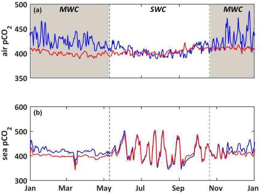
298                                     K. Lajaunie-Salla et al.: A carbonate system model in a Mediterranean coastal site

Figure 2. Map of study area: the Region Sud (a), Aix–Marseille Metropolis (area in the red rectangle) (b), the Bay of Marseille (c).
CAV = Cinq Avenues Station (urban site); OHP: Observatoire de Haute Provence station (non-urban site); Carry, Solemio, Planier: marine
study sites in the Bay of Marseille.

2.2   Study area                                                     (including CO2 ) from the nearby urban area, and it also re-
                                                                     ceives effluents from the Aix–Marseille metropolis.

The BoM is located in the eastern part of the Gulf of Lion,          2.3   Dataset
in the northwestern Mediterranean Sea (Fig. 2). The city of
Marseille, located on the coast of the BoM, is the second            The modeled variables of the carbonate system (DIC, TA,
largest city of France, with a population of ca. 1 million.          pH, and pCO2 ) and chlorophyll a are hereafter compared
The Rhône River, which flows into the Gulf of Lion, is the           to observations collected at the SOLEMIO station (Figs. 2c
greatest source of freshwater and nutrients for the Mediter-         and 3), which is a component of the French national moni-
ranean Sea, with a river mean flow of 1800 m3 s−1 (Pont              toring network (Service d’Observation en Milieu Littoral –
et al., 2002). Several studies highlight the eastward intru-         SOMLIT, http://somlit.epoc.u-bordeaux1.fr/fr/, last access:
sion events from the Rhône River plume in the BoM under              January 2020). Major biogeochemical parameters have been
east and southeasterly wind conditions, which favor biologi-         recorded since 1994. Carbonate chemistry variables (pH,
cal productivity (Fraysse et al., 2014; Gatti et al., 2006; Para     pCO2 , DIC, and TA), sampled every 2 weeks, have been
et al., 2010). The biogeochemistry of the BoM is complex             available since 2016.
and highly driven by hydrodynamics. For example, north–
northwesterly winds induce upwelling events which bring              2.4   Design of numerical experiments
cold and nutrient-rich waters upward (Fraysse et al., 2013).
Moreover, the oligotrophic Northern Current occasionally in-         In the present work, the Eco3M-CarbOx model was run for
trudes into the BoM (Petrenko, 2003; Ross et al., 2016).             the whole year of 2017. This year was chosen because in
   Despite the presence of several marine protected areas            situ data of carbonate systems (DIC, TA, pH, and pCO2 )
around the BoM (the Regional Park of Camargue, the Marine            are available for the whole year at the SOLEMIO station
protected area Côte Bleue, and the National Park of Calan-           (Fig. 2c). The biogeochemical variables were initialized us-
ques), it is strongly impacted by diverse anthropogenic forc-        ing in situ data from winter conditions (Table B1, Ap-
ing, because industrialized and urbanized areas are located          pendix B). The model was forced by time series of sea sur-
all along the coast. From the land, the BoM receives nutrients       face temperature and salinity, wind (at 10 m), light, and at-
and organic matter from the urban area of the Aix–Marseille          mospheric CO2 concentrations. The sea temperature time
metropolis (Millet et al., 2018), the industrialized area of         series is from in situ hourly data recorded at the Planier
Fos-sur-Mer (one of the biggest oil-based industry areas in          station (Fig. 2c). For salinity, hourly in situ data from the
Europe), and the Berre Lagoon, which is eutrophized (Gouze           SOLEMIO station and from the CARRY buoy were used
et al., 2008; Fig. 2c). From the atmosphere, the BoM is sub-         (Fig. 2c). Wind and light hourly time series were extracted
ject to fine-particle deposition and greenhouse gas emissions        from the WRF meteorological model at the SOLEMIO sta-

Geosci. Model Dev., 14, 295–321, 2021                                                   https://doi.org/10.5194/gmd-14-295-2021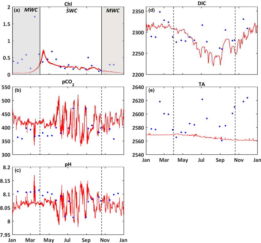
K. Lajaunie-Salla et al.: A carbonate system model in a Mediterranean coastal site                                                   299

Table 1. Forcing of the different scenarios (S) simulated with the model. See Sect. 2.4 for details of the scenarios.

                                       Temperature                      Wind                  River input    Atmospheric CO2
                S0 – Reference         In situ data of 2017             WRF model 2017        No             CAV station 2017
                S1 – T increases       In situ data of 2017 +1.5 ◦ C    WRF model 2017        No             CAV station 2017
                S2 – Wind constant     In situ data of 2017             7 m s−1               No             CAV station 2017
                S3 – Wind events       In situ data of 2017             3 d at 20 m s−1       No             CAV station 2017
                S4 – NO3               In situ data of 2017             WRF model 2017        Yes, NO3       CAV station 2017
                S5 – Non-urban         In situ data of 2017             WRF model 2017        No             OHP station 2017

tion (Yohia, 2017). Finally, we used hourly atmospheric CO2                      spheric CO2 values measured at the Observatoire de
values from in situ measurements recorded at the Cinq Av-                        Haute Provence station (OHP; Fig. 2b), located out-
enues station (CAV station; Fig. 2b) by the AtmoSud Re-                          side of the Aix–Marseille metropolis, by the ICOS
gional Atmospheric Survey Network, France (https://www.                          National Network, France (http://www.obs-hp.fr/ICOS/
atmosud.org, last access: August 2019). This simulation is                       Plaquette-ICOS-201407_lite.pdf, last access: August
the reference simulation (noted S0). As highlighted previ-                       2019).
ously, Rhône River plume intrusions (due to wind-specific
conditions) have an impact on the dynamics of primary pro-                   In this work, we calculated the daily mean values of state
duction (Fraysse et al., 2014; Ross et al., 2016) and then on             variables, statistical parameters, and mean fluxes of modeled
the seawater carbonate system. Moreover, the seawater tem-                processes throughout the year and over two main hydrolog-
perature and atmospheric CO2 variations control the seawa-                ical periods: the stratified and mixed water column periods.
ter CO2 dynamics via the solubility equilibrium and gas ex-               The stratified water column (SWC) is defined with a temper-
change with the atmosphere (Middelburg, 2019). In order to                ature difference between the surface and bottom of more than
quantify the impact of different forcing, several simulations             0.5 ◦ C (Monterey and Levitus, 1997). For the simulated year
(hereafter noted S), which are summarized in Table 1, were                (2017), the SWC period lasts from 10 May to 20 October.
conducted:                                                                The mixed water column (MWC) period corresponds to the
                                                                          rest of the year.
  – Impact of seawater temperature increase, S1. The forc-
    ing time series of in situ temperatures was shifted by
    +1.5 ◦ C (Cocco et al., 2013).                                        3     Results

  – Impact of wind events. A first simulation S2 was run                  3.1    Model skills
    with a constant wind intensity of 7 m s−1 (2017 annual
    average wind speed) throughout the year and a second                  Following the recommendations of Rykiel (1996), three cri-
    one (S3) with two three-day periods of strong wind                    teria were considered to evaluate the performance of our
    speed (20 m s−1 ) representative of short bursts of the               model:
    mistral (data not shown) starting on 15 May and 15 Au-                    – Does the model reproduce the timing of the ob-
    gust, and a constant value of 7 m s−1 the rest of the year.                 served variations of carbonate system at the seasonal
  – Impact of nutrient supply (nitrate) during a Rhône River                    timescale?
    plume intrusion (S4). A threshold of 37 has been chosen                   – Does the model reproduce the observed pCO2 and pH
    to identify the presence of low-salinity waters from the                    ranges at the seasonal timescale?
    Rhône River plume in the forcing file of salinity. Here,
    concentrations in nitrate supplied by the river depend on                 – Are the observations correctly represented according to
    the salinity. A relationship between these two variables                    the Willmott skill score (WSS)? This index is an objec-
    was then established for the SOLEMIO point from the                         tive measurement of the degree of agreement between
    MARS3D-RHOMA coupled physical and biogeochem-                               the modeled results and the observed data. A correct
    ical model (Fraysse et al., 2013; Pairaud et al., 2011).                    representation of observations by the model is achieved
    This relationship has already been used successfully to                     when this index is higher than 0.70 (Willmott, 1982).
    reproduce realistic observed conditions in the studies of
    Fraysse et al. (2014) and Ross et al. (2016): NO3intrusion              Over most of the studied period, the model simulates lower
    (mmol m−3 ) = −1.70 × S + 65.                                         chlorophyll a concentrations than the in situ observations, es-
                                                                          pecially during the MWC period (Fig. 3a). Two maxima of
  – Non-urban atmospheric CO2 concentrations (S5). This                   chlorophyll a concentrations are observed in situ: the first
    simulation takes into account the forcing of atmo-                    one at ca. 1.71 mg m−3 in March and the second one at ca.

https://doi.org/10.5194/gmd-14-295-2021                                                          Geosci. Model Dev., 14, 295–321, 2021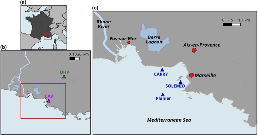
300                                             K. Lajaunie-Salla et al.: A carbonate system model in a Mediterranean coastal site

Figure 3. Comparison of model results (red) and in situ data (blue) at the surface of the SOLEMIO station. (a) Chlorophyll a concentrations
(mg m−3 ), (b) pCO2 (µatm), (c) pH, (d) DIC (µmol kg−1 ), (e) TA (µmol kg−1 ). The value of each state variable represents the mean around
± 5 d of the seawater sampling date. The shaded area and dotted black line delimit the SWC and MWC periods.

Table 2. Statistical evaluation of observations vs. model for 2017: observed and simulated minimum and maximum values. WSS = Willmott
skill score; N = number of measurements. Units of bias are those of modeled variables: chlorophyll a (Chl a, mg m−3 ), seawater partial
pressure of CO2 (seawater pCO2 , µatm), pH, dissolved inorganic carbon (DIC, µmol kg−1 ), and total alkalinity (TA, µmol kg−1 ).

                                                   Chl a   Seawater pCO2             pH           DIC              TA
                    Obs. min–max           [0.10–1.71]         [358–471]   [8.014–8.114]   [2260–2348]    [2561–2624]
                    Mod. min–max           [0.03–0.73]         [331–522]   [7.979–8.171]   [2220–2323]    [2560–2572]
                    Bias                        −0.22              22.47         −0.016          −8.48         −24.91
                    WSS                           0.36             0.69∗           0.75∗         0.71∗           0.43
                    N                               22                20              21            20             20
                  ∗ Significant value of WSS (> 0.70).

0.68 mg m−3 in May. They are both linked to Rhône River                    titatively reproduces the spring bloom observed at the end
plume intrusions. Several in situ maxima between 0.50 and                  of the MWC period (Fig. 3a) with a maximum value of ca.
0.70 mg m−3 are observed between March and April (at the                   0.69 mg m−3 . The model does not catch the two aforemen-
end of the MWC period), and they signaled the spring bloom                 tioned maxima of chlorophyll, and it contains a low WSS
event (Table 2 and Fig. 3a). The biogeochemical model quan-

Geosci. Model Dev., 14, 295–321, 2021                                                       https://doi.org/10.5194/gmd-14-295-2021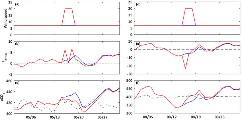
K. Lajaunie-Salla et al.: A carbonate system model in a Mediterranean coastal site 301
and a strong bias (0.37 and +0.22 mg m−3 , respectively – Ta- 3.2 Carbon fluxes and budgets
ble 2).
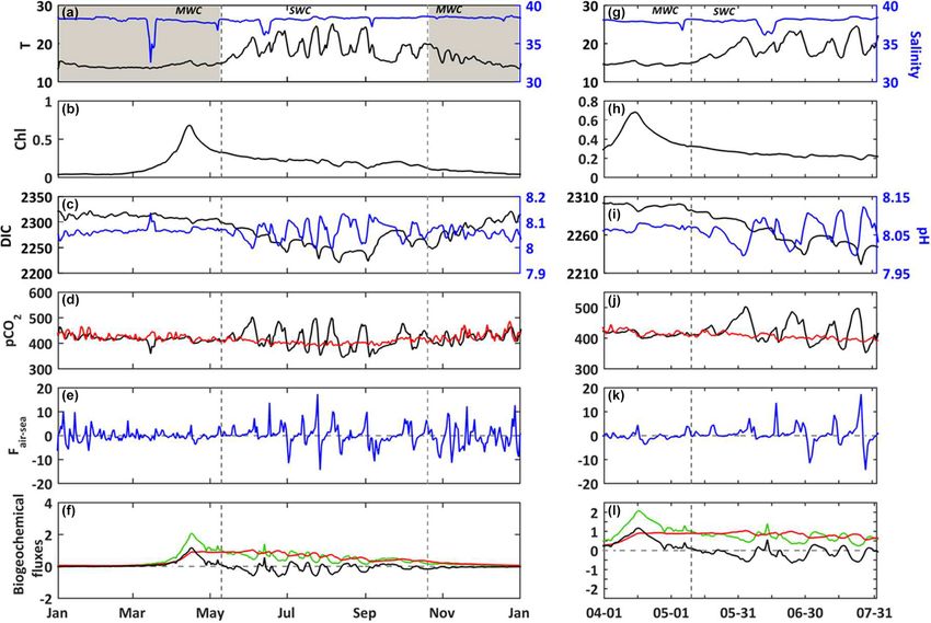
On the whole, the seasonal variations of the seawater For the year 2017, the values of temperature vary between
pCO2 are correctly simulated by the biogeochemical model 13.3 and 25.9 ◦ C (Fig. 4a). The DIC variations closely match
(Fig. 3b), even if the values are rather overestimated during those of temperature (correlation coefficient −0.75). For ex-
the MWC period. From January to February, the model re- ample, the spring increase in temperature leads to a decrease
produces the slight decrease in the observed pCO2 , and from in DIC concentrations (Fig. 4a and c), and the minimum val-
February to March it reproduces the increase in pCO2 even if ues are reached at the end of SWC period. Over the simu-
the amplitude of this increase remains smaller. In mid-April, lated period, the air–sea CO2 fluxes (Faera ) vary between −14
during the simulated spring bloom period, the observed drop and 17 mmol m−3 d−1 , with a weakly positive annual budget
in pCO2 and increase in pH are also spotted in the model of +6 mmol m−3 yr−1 (or +0.017 mmol m−3 d−1 , Table 3).
(Fig. 3b and c). The model especially succeeds in reproduc- Then, the BoM waters would act as a net source of CO2 to
ing the observed increase in relation to high temperatures the atmosphere on an annual basis. However, on a seasonal
during the SWC period. The reduction of the CO2 solubility basis, the BoM waters would change from a net sink during
due to thermal effects mostly explains the increase in pCO2 the MWC period (Faera < 0; Table 3) to a net source during
during the SWC period. The strong SD of modeled values the SWC one (Faera > 0; Table 3).
during the SWC period can be explained by the rapid changes On an annual basis, the gross primary production (GPP)
in temperature, probably due to upwelling usually occurring and total respiration (R) are balanced, leading to a null
at this time of the year (Millot, 1990). The range of modeled average net ecosystem production (NEP; NEP = GPP−R)
pCO2 values (345–503 µatm) encompasses the range of ob- (Fig. 4f and Table 3). The intensity of autotrophic respiration
served values (358–471 µatm; Table 2). The statistical anal- (Ra ) is lower than that of primary production (annual mean
ysis provides a mean bias of +23 µatm, and a WSS of 0.69 of 0.065 vs. −0.413 mmol m−3 d−1 , respectively – Table 3),
(Table 2). while the zooplankton and bacterial respiration account for
The seasonal dynamic of pH is mostly reproduced by the an average of 0.348 mmol m−3 d−1 (Table 3). On a seasonal
model, and in particular, the decrease during the SWC period basis, the model highlights an ecosystem dominated by au-
(Fig. 3c). However, the modeled pH is generally underesti- totrophy during the MWC period (NEP > 0; Table 3) and
mated throughout the year, except during the SWC period, heterotrophy during the SWC period with higher flux val-
with a mean bias of −0.015 (Table 2). The seasonal range ues (NEP < 0; Table 3). The biogeochemical fluxes show the
is captured by the model with a minimum value during the strongest variations along the SWC period, following those
SWC period (7.994 vs. 8.014 for observations; Table 2) and of temperature (Fig. 4f). The maximum GPP occurs in April
a maximum one during the MWC period (8.137 vs. 8.114 for and is correlated with the maximum chlorophyll concentra-
observations; Table 2). The statistical analysis highlights an tion. At this time, the ecosystem is autotrophic (NEP > 0;
index of agreement between the in situ data and the model Fig. 4b and f) and is a net sink for atmospheric CO2 , which
outputs higher than 0.70 (Table 2). explains the DIC and seawater pCO2 decreases during the
The seasonal variations of DIC show the highest values bloom period (Fig. 4c–e)
during the MWC period and a decrease (increase) during the When looking in detail at the 2017 temperature and salin-
beginning (the end) of the SWC period (Fig. 3d). The lowest ity time series (Fig. 4a), several crucial events can be seen oc-
values are observed during September. The Eco3M-CarbOx curring, including freshwater intrusions (e.g., 15 March and
model closely matches the seasonal dynamic by reproducing 6 May) into the BoM and large variations of temperature in
the range of extreme observed values (Table 2). The mean relation to upwelling events or latent heat losses due to wind
bias is also small (−8.48 µmol kg−1 ; Table 2). More than bursts. The largest freshwater intrusion from the Rhône River
70 % (0.73; Table 2) of modeled DIC concentrations are in plume occurs in mid-March, with a minimum observed salin-
statistical agreement with the corresponding observations. ity of ca. 32.5 at the SOLEMIO station (Fig. 4a). During this
The seasonal cycle of measured TA does not show a clear event, the seawater pCO2 decreases and pH increases con-
pattern (Fig. 3e). Large variations of values ranging between comitantly (Fig. 4c and d). Then, seawater appears to be tem-
2561 and 2624 µmol kg−1 (Table 2) are observed, what- porarily under-saturated in CO2 , and the BoM waters thus
ever the hydrological season being considered. The biogeo- act as a sink for atmospheric CO2 at the time of intrusion
chemical model provides almost constant values of around (Fig. 4e).
2570 µmol kg−1 all throughout the year, which is lower than During the SWC period, upwelling events quickly cool the
in situ data. With a low WSS index of agreement and a large surface seawater. In two days, from 25 to 27 July, the wa-
mean bias (Table 2), the model is not able to confidently re- ter temperature drops from 24.7 to 16.9 ◦ C (Fig. 4g). The
produce the observed variations of TA (Fig. 3e and Table 2). decrease in temperature corresponds to the increase in DIC
concentrations (Fig. 4i). Concomitantly, the value of seawa-
ter pCO2 decreases from 497 to 352 µatm, and pH increases
from 7.99 to 8.12 (Fig. 4i and j). This event quickly changes
https://doi.org/10.5194/gmd-14-295-2021 Geosci. Model Dev., 14, 295–321, 2021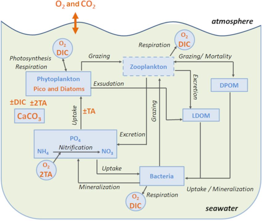
302                                           K. Lajaunie-Salla et al.: A carbonate system model in a Mediterranean coastal site

Figure 4. (a–f) 2017. (g–l) Temporal focus between 1 April and 31 July 2017. In situ daily average of (a, g) temperature (◦ C, black line)
and salinity (blue line) at the SOLEMIO station (at the surface). Modeled daily average (b, h) chlorophyll a concentrations (mg m−3 , black
line) (c, i) DIC (µmol kg−1 , black line) and pH (blue line), (d, j) seawater pCO2 (µatm, black line) and atmosphere pCO2 from OHP
(µatm, red line), (e, k) air–sea CO2 fluxes (mmol m−3 d−1 ), (f, l) gross primary production (mmol m−3 d−1 , green line), total respiration
(mmol m−3 d−1 , red line) and net ecosystem production (mmol m−3 d−1 , black line). The shaded areas and dotted black lines delimit the
SWC and MWC periods.

Table 3. Mean flux values (mmol m−3 d−1 ) and the contribution of each process to the DIC variations for the reference simulation over the
year and SWC/MWC periods.

                                                             Aeration           GPP          RA         RH            R         NEP
                            Mean flux           Year           0.017        −0.413        0.065       0.348      0.413            0
                                                MWC           −0.245        −0.314        0.052       0.176      0.228        0.086
                                                SWC            0.405        −0.521        0.079       0.555      0.634       −0.113
                            Contribution        Year             78 %          11 %          2%         9%        11 %               –
                          GPP: gross primary production, RA : autotrophic respiration, RH : heterotrophic respiration, NEP: net ecosystem
                          production.

Geosci. Model Dev., 14, 295–321, 2021                                                                         https://doi.org/10.5194/gmd-14-295-2021
K. Lajaunie-Salla et al.: A carbonate system model in a Mediterranean coastal site 303
the BoM waters from a source to a sink for atmospheric CO2 period of the spring sink to extend by ca. 3 weeks over May
(from +17 to −14 mmol m−3 d−1 ; Fig. 4k), and also from a relative to the reference simulation (Fig. 5j).
net heterotrophic to a net autotrophic ecosystem (Fig. 4l).
3.3.2 Wind speed
3.3 Impact of external forcing on the dynamics of
carbonate system The Bay of Marseille is periodically under the influence of
strong wind events (Millot, 1990). Here we compare two
3.3.1 Temperature increase simulations: one with a constant wind value (S2) and the
other one with two wind events that occur in May and August
Here we compare the reference simulation S0 with the (S3) (Fig. 6a and d). The result of this numerical experiment
S1 simulation (seawater temperature elevation of 1.5 ◦ C – shows that the stronger the wind speed is, the higher the air–
Fig. 5). During the year, there are few changes on the car- sea fluxes are, mainly owing to the increase in gas transfer
bonate system variables such as the pCO2 and pH (data not velocity. Depending on the gradient of CO2 between seawa-
shown). The main alterations occur during the blooms of ter and the atmosphere, strong wind speeds will favor either
phytoplankton. The simulated bloom of phytoplankton oc- the emission or uptake of CO2 (Fig. 6b and e). In May, with
curs later, at beginning of May, for both diatoms and pico- the air–sea CO2 flux being positive, the outgassing of CO2 to
phytoplankton, with maximum values of chlorophyll at 1.4 the atmosphere is enhanced, leading to a decrease in seawater
and 0.4 mg m−3 , respectively (Fig. 5a and f). pCO2 (Fig. 6c). On the contrary, in August the oceanic sink
As both the limitations due to light and nutrients remain of atmospheric CO2 is amplified, which leads to an increase
about the same during the simulations S0 and S1, this coun- in the seawater pCO2 value (Fig. 6f).
terintuitive occurrence of a bloom relative to changes in
3.3.3 Supply in nitrate by river inputs
temperature is mainly explained by the temperature limit-
ing function, which depends on the optimal temperature of According to the model results (Fig. 7), the occasional in-
growth (Topt ). For the picophytoplankton, from January to puts of nitrate (S4) that are linked to Rhône River plume in-
April, the increase of 1.5 ◦ C drastically reduces the limitation trusions favor primary production, and they led to increased
by temperature (Fig. 5c), because the temperature is closer to chlorophyll concentrations (Fig. 7b and c) five times during
the optimal temperature (Topt = 16 ◦ C, Table A4) during S1 the SWC period. These blooms, as seen previously, lead to
than S0. In the S0 simulation, the temperature reaches Topt a decrease (increase) in the seawater pCO2 (pH) (Fig. 7e
ca. 15 April and it induces the bloom, while at the same time and f). It can be noted that with the strongest river supply
in S1 the temperature moves slightly away from Topt and it at mid-March (Fig. 7a and b) the occurrence of the spring
does not enable the triggering of a bloom. At the time of the bloom is earlier (Fig. 7c) than that occurring in the reference
bloom in S1, the opposite configuration occurs. In S0, the simulation (S0). The time lag between river nutrient supply
ambient temperature is again far from Topt , explaining the and bloom is due to the temperature limitation (Fig. 4c). Dur-
absence of a bloom, while in the S1 the ambient temperature ing blooms occurring within the SWC period following intru-
is closer to Topt , enabling the occurrence of a bloom. The sions, the DIC concentrations are generally lower than those
picophytoplankton bloom then occurs later in the warm sim- of the reference simulation, as in the case of the bloom of
ulation S1 than in the reference simulation S0 (Fig. 5a). The mid-May (decrease by ca. 15 µmol kg−1 ; Fig. 7j), due to the
duration and termination of a bloom is controlled by both autotrophic processes dominating the heterotrophic ones. In
the nutrient availability and the temperature (Fig. 5c and d). turn, the seawater pCO2 drops by ca. 30 µatm (Fig. 7k) and
Inversely, from January to April, the diatoms’ growth lim- pH increases by ca. 0.030 (Fig. 7l). Nitrate inputs, favoring
itation by temperature is strengthened in the warm simula- primary production, reduce the source of CO2 to the atmo-
tion S1 (Fig. 5h), because the resulting ambient temperature sphere and intensify the sink of atmospheric CO2 into the
is further from the optimum temperature (Topt = 13 ◦ C, Ta- waters of BoM (Fig. 7e and k).
ble A4) than that in the reference simulation S0. This induces
a slower growth of diatoms and a delay of the maximum con- 3.3.4 Urban air CO2 concentrations
centration (Fig. 5f). Afterwards the photosynthesis is mainly
limited by temperature (Fig. 5h). The Aix–Marseille metropolis is strongly subject to urban
The ecosystem is dominated by autotrophs at the time emissions to the atmosphere (Xueref-Remy et al., 2018a).
of blooms whatever the simulation considered (NEP > 0; The seasonal variability of atmospheric CO2 concentrations
Fig. 5e), and the quantity of DIC (not shown) fixed through at the urban site (CAV station; Fig. 2) is much higher than
autotrophic processes is larger than that released by het- that observed in a non-urban area (OHP station; Fig. 2), es-
erotrophic processes. During the short period of a bloom, pecially during the MWC period (Fig. 8a): CO2 concentra-
the seawater pCO2 decreases, leading to some negative air– tions vary between 379 and 547 µatm at the CAV station and
sea fluxes (i.e., an oceanic sink for atmospheric CO2 ). In the between 381 and 429 µatm at the OHP station. Moreover, in
warm simulation, the later occurrence of a bloom enables the winter the atmospheric pCO2 is higher in the urban area than
https://doi.org/10.5194/gmd-14-295-2021 Geosci. Model Dev., 14, 295–321, 2021304 K. Lajaunie-Salla et al.: A carbonate system model in a Mediterranean coastal site
Figure 5. Modeled daily average chlorophyll a concentrations (mg m−3 ) (a), light limitation (b), temperature limitation, and a close-up from
15 April to 5 May of temperature (c) and nutrient limitation (d) for picophytoplankton and the same set for diatoms (f–i). Modeled daily
average NEP (mmol m−3 d−1 , e) and air–sea CO2 fluxes (mmol m−3 d−1 , j). Reference simulation (S0, blue line) and temperature-shifted
simulation by 1.5 ◦ C (S2, red line). The shaded area and dotted black lines delimit the SWC and MWC periods.
the non-urban area, whereas in summer those of both areas 4 Discussion
are quite close. These differences in the seasonal pattern and
between areas are usually explained by (i) the thinner atmo- 4.1 Model performance
spheric boundary layer, (ii) the decreased fixation of CO2 by
terrestrial vegetation, and (iii) the greater influence of anthro-
The evaluation of model skill vs. in situ data highlights that
pogenic activities by emissions from heating (Xueref-Remy
the modeled pH, pCO2 , and DIC are in acceptable agreement
et al., 2018b). Forcing the model by atmospheric pCO2 val-
with observations (Fig. 3). The seasonal variations observed
ues from urban or non-urban sites can lead to significant dif-
for the different variables are captured by the model, includ-
ferences in the values of the seawater pCO2 , especially dur-
ing for example the seasonal decrease in DIC and pH during
ing the MWC period. The air–sea gradient of pCO2 is higher
the SWC period, in relation to the increase in pCO2 , and
when using a forcing derived from the CO2 concentrations
the inverse scenario during the MWC period. The chloro-
originating from an urban area than from a non-urban area,
phyll content variability is not well reproduced, especially
which strengthens the sink of atmospheric CO2 into the wa-
during spring (Fig. 3a), even taking into account the nitrate
ters of BoM. The seawater pCO2 is then lower with non-
supply from the Rhône River plume intrusion (Fig. 7c). This
urban area pressure (S5) than with urban area pressure (S0),
is due to the multiple origins of chlorophyll, organic mat-
because of lower CO2 solubility in the BoM (Fig. 8b).
ter, and nutrients in the BoM that are not accounted for in
the Eco3M-CarbOx model: autochthonous marine produc-
tion, and allochthonous origins from the Rhône and Hu-
veaune River plumes (Fraysse et al., 2013). The observed
variations and levels of TA are not correctly simulated by the
model (Fig. 3f). The study of Soetaert et al. (2007) highlights
Geosci. Model Dev., 14, 295–321, 2021 https://doi.org/10.5194/gmd-14-295-2021K. Lajaunie-Salla et al.: A carbonate system model in a Mediterranean coastal site 305
Figure 6. Temporal evolution for May (a–c) and August (d–f) 2017 of the wind speed (m s−1 , a, d); air–sea CO2 fluxes (mmol m−3 d−1 , b,
e); seawater pCO2 (µatm, c, f). Constant wind scenario (S2, blue line) and wind event scenario (S3, red line). On (c) and (f), the dashed line
represents the atmosphere pCO2 (µatm) at the CAV station.
that the main variations of TA in the marine coastal zones crease in the pCO2 level. The imbalance between the latter
are linked to freshwater supplies and marine sediments. The two processes leads to a change in the ecosystem status (au-
present study does not take into account the inputs of TA totrophic or heterotrophic) and the corresponding behavior
from the Rhône River and the water–sediment interface, and as a sink or source to the atmosphere. In case of a 1.5 ◦ C
it may explain why the TA variable is not correctly predicted rise over the whole year, the temperature variation has a very
by our model. small impact on the carbonate system dynamics. However, it
favors the autotrophic processes and strengthens the oceanic
4.2 Contribution of physical and biogeochemical sink of atmospheric CO2 during the bloom of phytoplankton
processes to the variability of carbonate system (Fig. 5e and j).
The contribution of each biogeochemical process to the DIC 4.3 Contribution of the external forcing to the
variability can be assessed using the presented model: the variability of carbonate system
aeration process contributes to 78 % of the DIC variations,
and all biogeochemical processes together contribute to 22 % In line with several previous works on the northwestern
(Table 3). As mentioned by Wimart-Rousseau et al. (2020), Mediterranean Sea (De Carlo et al., 2013; Copin-Montégut
the model suggests that the seawater pCO2 variations and as- et al., 2004; Wimart-Rousseau et al., 2020), the model also
sociated fluxes would be mostly driven by the seawater tem- suggests that the status of the Bay of Marseille regarding
perature dynamics. Moreover, the seasonal variations of the sink or source for CO2 could change at high temporal fre-
air–sea CO2 flux are in agreement with some previous field quency (i.e., hours to days). Bursts of north–northwestern
studies (De Carlo et al., 2013; Wimart-Rousseau et al., 2020), winds lead to sudden and sharp decreases in seawater tem-
which measured a weak oceanic sink for atmospheric CO2 perature (< 2 d; Fig. 4g) either directly by latent heat loss
during winter and a weak source to the atmosphere during through evaporation at the surface (Herrmann et al., 2011)
summer. or indirectly by creating upwelling (Millot, 1990), with the
The model results reveal that temperature would play a consequences of a decrease in the seawater pCO2 values
crucial role in controlling two counterbalanced processes: (Fig. 4j) and, in fine, an alteration of the CO2 air–sea fluxes.
(1) the carbonate system equilibrium and (2) the phytoplank- Model results suggest that the fast variations of tempera-
ton growth. The increase in temperature during SWC leads ture could lead to rapid changes of the sink vs. source sta-
to a higher pCO2 in seawater due to the decrease in the CO2 tus in this coastal zone (Fig. 4k). Moreover, Fraysse et al.
solubility (Middelburg, 2019) and, at the same time, the fix- (2013) highlight that upwelling in the BoM favors ephemeral
ation of DIC by phytoplankton is favored, leading to a de- blooms of phytoplankton by nutrient supplies up to the eu-
https://doi.org/10.5194/gmd-14-295-2021 Geosci. Model Dev., 14, 295–321, 2021306 K. Lajaunie-Salla et al.: A carbonate system model in a Mediterranean coastal site Figure 7. (a–f) 2017. (g–l) Temporal focus between 1 May and 1 July 2017. (a, g) In situ daily average of salinity. Modeled daily average (b, h) nitrate concentrations (mmol m−3 ); (c, i) chlorophyll a concentrations (mg m−3 ); (d, j) DIC (µmol kg−1 ); (e, k) seawater pCO2 (µatm); and (f, l) pH. Reference simulation (S0, blue line) and nitrate supply simulation (S4, red line). On (e) and (k), the dashed line represents the atmosphere pCO2 (µatm) at the CAV station. The shaded area and dotted black lines delimit the SWC and MWC periods. photic layer and would, in turn, contribute to the seawater nificant impact on the seawaterpCO2 values during a longer pCO2 decrease. North and northwestern winds through la- period of ca. 15 d (Fig. 6). A combination of high atmo- tent heat losses and/or upwelling events could then enhance spheric pCO2 values and high wind speeds would then favor the sink for atmospheric CO2 due to the temperature drop the sink for CO2 into the waters of the BoM. The aeration and nutrients inputs. However, these results remain prelim- process also depends on the choice of the formulation of the inary because in our experimental design only the cooling gas transfer velocity (k600 ). In this study, the formulation of effect of upwelling on the carbonate balance is taken into ac- Wanninkhof (1992) is used and depends of the wind speed count. But concomitantly, upwelling usually bring nutrients at 10 m above the water surface. However, the current veloc- and DIC at the surface and these supplies could also perturb ity could favor the gas exchange, and suspended matter con- the balance of the carbonate system. A further coupling of centration could limit the gas exchange (Abril et al., 2009; the Eco3M-CarbOx model with a tridimensional hydrody- Upstill-Goddard, 2006; Zappa et al., 2003). Due to the im- namic model would certainly enable the multiple effects of portant heterogeneity of physical and biogeochemical forc- upwelling on the dynamics of the carbonate system in this ings in coastal zones, other factors that control the air–sea area to be embraced and the results presented in this study to gas exchange should certainly be taken into account. be refined. The simulation with intrusions of the Rhône River plume High wind speeds (> 7 m s−1 ) amplified the gaseous ex- shows that inputs of nitrate cause a drop of seawater pCO2 change of CO2 considerably (De Carlo et al., 2013; Copin- owing to the nutrient supply favoring the phytoplankton de- Montégut et al., 2004; Wimart-Rousseau et al., 2020). The velopment (Fig. 7). In this scenario, the oceanic sink of at- model highlights that a strong wind event of 3 d has a sig- mospheric CO2 is enhanced. But rivers also supply TA (e.g., Geosci. Model Dev., 14, 295–321, 2021 https://doi.org/10.5194/gmd-14-295-2021
K. Lajaunie-Salla et al.: A carbonate system model in a Mediterranean coastal site                                                 307

                                                                        against in situ data available in the Bay of Marseille (north-
                                                                        western Mediterranean Sea) over the year 2017. The model
                                                                        correctly simulates the value ranges and seasonal dynam-
                                                                        ics of most of the variables of the carbonate system except
                                                                        for the total alkalinity. Several numerical experiments were
                                                                        also conducted to test the sensitivity of the carbon balance to
                                                                        physical processes (temperature and salinity), biogeochemi-
                                                                        cal processes (GPP and respiration processes), and external
                                                                        forcing (wind, river intrusion, and atmospheric CO2 ). This
                                                                        set of numerical experiments shows that the Eco3M-CarbOx
                                                                        model provides expected responses in the alteration of the
                                                                        marine carbonate balance regarding each of the considered
                                                                        perturbation.
                                                                           On the whole, the model results suggest that the carbonate
                                                                        system is mainly driven by the seawater temperature dynam-
                                                                        ics. At a seasonal scale, the BoM marine waters appear to be
Figure 8. (a) Temporal evolution for the year 2017 of the observed
                                                                        a net sink of atmospheric CO2 and a dominantly autotrophic
pCO2 (µatm) in the atmosphere at the CAV station, called the “ur-
ban scenario” (S0, blue line), and at the OHP station, called the
                                                                        ecosystem during the MWC period, and a net source of CO2
“non-urban scenario” (S6, red line). (b) Temporal evolution for the     to the atmosphere during the SWC period, which is mainly
year 2017 of the modeled seawater pCO2 (µatm) with forcings from        characterized by a dominance of heterotrophic processes.
the urban (S0, blue line) and non-urban (S6, red line) scenarios. The   However, the model results highlight that sharp seawater
shaded area and dotted black lines delimit the SWC and MWC pe-          cooling observed within the SWC period, probably owing
riods.                                                                  to upwelling events, cause the CO2 status of the BoM ma-
                                                                        rine waters to change from a source to the atmosphere to a
                                                                        sink into the ocean within a few days. External forcing as the
Gemayel et al., 2015; Schneider et al., 2007) and DIC (e.g.,            temperature increases leads to a delay in the bloom of phy-
Sempéré et al., 2000) that shift the carbonate system equilib-          toplankton. Strong wind events enhance the gas exchange of
rium toward a pCO2 decrease and a DIC increase (Middel-                 CO2 with the atmosphere. A Rhône River plume intrusion
burg, 2019). Taking into account these further supplies may             with input of nitrate favors pCO2 decreases, and the sink
sensibly modify the modeled carbonate balance in the BoM.               of atmospheric CO2 into the BoM waters is enhanced. The
A next step to the present work will be to design more realis-          higher atmospheric pCO2 values from the urban area inten-
tic numerical experiments to refine the results obtained in this        sify the oceanic sink of atmospheric CO2 .
preliminary study. The intrusions of the Rhône River plume                 The BoM biogeochemical functioning is mainly forced by
also induce a salinity decrease in the BoM waters, which                wind-driven hydrodynamics (upwelling, downwelling), ur-
leads to a drop in the pCO2 levels in the model. This drop              ban rivers, wastewater treatment plants, and atmospheric de-
of pCO2 is due to the decrease in the CO2 solubility when               position (Fraysse et al., 2013). In addition, Northern Cur-
salinity decreases (Middelburg, 2019).                                  rent and Rhône River plume intrusions frequently occurred
   In the scenario of forcing the model by using urban atmo-            (Fraysse et al., 2014; Ross et al., 2016). Moreover, the BoM
spheric pCO2 time series, the air–sea gradient increases, and           harbors the second biggest metropolis of France (Marseille),
then it enhances the status of the BoM as a sink for atmo-              which is impacted by many harbor activities. The next step
spheric CO2 . As suggested by the in situ study of Wimart-              of this study will be to couple the Eco3M-CarbOx biogeo-
Rousseau et al. (2020), the Eco3M-Carbox model highlights               chemical model to a 3-D hydrodynamic model that will mir-
the crucial role of the coastal ocean in an urbanized area, and         ror the complexity of the BoM functioning. In this way, the
with an increase in atmospheric CO2 , the CO2 uptake by the             contributions of hydrodynamic, atmospheric, anthropic, and
coastal ocean may increase. This result is in line with the             biogeochemical processes to the DIC variability will be able
studies of Andersson and Mackenzie (2004) and Cai (2011),               to be determined with higher refinement and realism, and an
which predict an increase in the intensity of the CO2 sink and          overview of the air–sea CO2 exchange could be made at the
a potential threat to coastal marine biodiversity in coastal ar-        scale of the Bay of Marseille. The main results of our study
eas owing to high atmospheric CO2 levels.                               could be transposed to other coastal sites that are also im-
                                                                        pacted by urban and anthropic pressures. Moreover, in this
                                                                        paper we highlighted that fast and strong variations of pCO2
5   Conclusions                                                         values occur, and thus it is essential to acquire more in situ
                                                                        values at high frequency (at least with an hourly resolution)
A marine carbonate chemistry module was implemented in                  to understand the rapid variations of the marine carbon sys-
the Eco3M-CarbOx biogeochemical model and evaluated                     tem at these short spatial and temporal scales.

https://doi.org/10.5194/gmd-14-295-2021                                                     Geosci. Model Dev., 14, 295–321, 2021
308 K. Lajaunie-Salla et al.: A carbonate system model in a Mediterranean coastal site
Appendix A: Details of resolution of carbonate system
module −4276.1
KS = + 141.328 − 23.093 · log(T(K) )
A1 Calculation of carbonate system constants T(K)
13856
The concentrations in conservative elements (relative to + 324.57 − 47.986 · log(T(K) ) −
T(K)
salinity) are calculated as follows:
· Ions2 ,
– Total fluoride (TF) concentrations from Riley (1965)
in mol kg−1 : KS = KS + − 771.54 + 114.723 · log(T(K) )
0.000067 S 35 474 −2698 3 1776
TF = · . + · Ions + · Ions 2 +
18.998 1.80655 T(K) T(K) T(K)
· Ions2 ,
– Total sulfate (TS) concentration from Morris and Riley
(1966) in mol kg−1 : KS = eKS ·(1−0.001005·S) ;
0.14 S – KF equilibrium constant of dissociation of hydrogen
TS = · .
96.062 1.80655 fluoride (HF) formation from Dickson and Riley (1979)
in mol kg−1 :
– Calcium ion concentration from Riley and Tongudai
1
(1967) in mol kg−1 : 1590.2
T(K) −12.641+1.525·Ions
2
KF = e · (1 − 0.001005 · S) ;
0.02128 S
Ca2+ = · . – KB equilibrium constant of dissociation of boric acid
40.087 1.80655
from Dickson (1990b) in mol kg−1 :
– Total boron (TB) concentration from Uppström (1974) 1
in mol kg−1 : KB = − 8966.9 − 2890.53 · S 2 − 77.942 · S
3
+ 1.728 · S 2 − 0.0996 · S 2 /T(K) ,
0.000416 · S
TB = . 1
35 KB = KB + 148.0248 + 137.1942 · S 2 + 1.62142 · S
1
– Ionic strength (IonS) from Millero (1982): + (−24.4344 − 25.085 · S 2 − 0.2474 · S)
1
19.924 · S · log(T ) + 0.053105 · S 2 · T ;
IonS = .
1000 − 1.005 · S – K0 constant of CO2 solubility from Weiss (1974)
in mol kg−1 atm−1 :
The constants are calculated on the total pH scale except
for KS on free pH scale. If necessary, pH scale conversion 100
factors are as follows: K0 = exp − 60.2409 + 93.4517 · + 23.3585
T(K)
– From seawater pH scale (SWS) to total pH scale: T(K) T(K)
TS
· log + S · 0.023517 − 0.023656 ·
1+ K
S
100 100
SWStoTOT = TS ;
1+ K + KTF 2
S F T(K)
+ 0.0047036 · ;
– From free pH scale to total pH scale: FREEtoTOT = 100
TS
1+ K S
.
– Ke dissociation constant of water from Millero (1995)
Further carbonate system constants were calculated as fol- in (mol kg−1 )2 :
lows:
−13847.26
Ke = exp + 148.9802 − 23.6521
– KS equilibrium constant of dissociation of HSO−
4 from
T(K)
Dickson (1990a) in mol kg−1 :
118.67
· log(T(K) ) + − 5.977 + + 1.0495
T(K)
1
· log(T(K) ) · S 2 − 0.01615 · S ,
Ke = Ke · SWStoTOT, on total pH scale in mol kg−1 ;
Geosci. Model Dev., 14, 295–321, 2021 https://doi.org/10.5194/gmd-14-295-2021You can also read