Changing sources and processes sustaining surface CO2 and CH4 fluxes along a tropical river to reservoir system - Biogeosciences
←
→
Page content transcription
If your browser does not render page correctly, please read the page content below
Biogeosciences, 18, 1333–1350, 2021
https://doi.org/10.5194/bg-18-1333-2021
© Author(s) 2021. This work is distributed under
the Creative Commons Attribution 4.0 License.

Changing sources and processes sustaining surface CO2 and CH4
fluxes along a tropical river to reservoir system
Cynthia Soued and Yves T. Prairie
Groupe de Recherche Interuniversitaire en Limnologie et en Environnement Aquatique (GRIL), Département des Sciences
Biologiques, Université du Québec à Montréal, Montréal, H2X 3X8, Canada

Correspondence: Cynthia Soued (cynthia.soued@gmail.com)

Received: 6 July 2020 – Discussion started: 14 September 2020
Revised: 15 January 2021 – Accepted: 18 January 2021 – Published: 22 February 2021

Abstract. Freshwaters are important emitters of carbon diox-    1   Introduction
ide (CO2 ) and methane (CH4 ), two potent greenhouse gases
(GHGs). While aquatic surface GHG fluxes have been ex-          Surface inland waters are globally significant sources of
tensively measured, there is much less information about        greenhouse gases (GHGs) to the atmosphere, namely carbon
their underlying sources. In lakes and reservoirs, surface      dioxide (CO2 ) and methane (CH4 ) (Bastviken et al., 2011;
GHG can originate from horizontal riverine flow, the hy-        DelSontro et al., 2018a; Raymond et al., 2013). Freshwa-
polimnion, littoral sediments, and water column metabolism.     ters act as both transport vessels for terrestrial carbon (C)
These sources are generally studied separately, leading to      and as active biogeochemical processors, making them key
a fragmented assessment of their relative role in sustaining    sites of GHG exchange with the atmosphere (Tranvik et al.,
CO2 and CH4 surface fluxes. In this study, we quantified        2018). The impoundment of rivers for hydropower gener-
sources and sinks of CO2 and CH4 in the epilimnion along        ation, irrigation, flood control, or other purposes changes
a hydrological continuum in a permanently stratified tropical   the landscape and its C cycling (Maavara et al., 2017), of-
reservoir (Borneo). Results showed that horizontal inputs are   ten resulting in increased aquatic CO2 and CH4 emissions
an important source of both CO2 and CH4 (> 90 % of sur-         due to the decay of flooded organic matter (Prairie et al.,
face emissions) in the upstream reservoir branches. However,    2018; Venkiteswaran et al., 2013). Globally, reservoirs are
this contribution fades along the hydrological continuum, be-   estimated to emit between 0.5 and 2.3 PgCO2 eq yr−1 (Bar-
coming negligible in the main basin of the reservoir, where     ros et al., 2011; Bastviken et al., 2011; Deemer et al., 2016;
CO2 and CH4 are uncoupled and driven by different pro-          St. Louis et al., 2000), and this number is predicted to in-
cesses. In the main basin, vertical CO2 inputs and sediment     crease with a rapid growth of the hydroelectric sector in the
CH4 inputs contributed to on average 60 % and 23 % respec-      upcoming decades (Zarfl et al., 2015). Several studies have
tively to the surface fluxes of the corresponding gas. Water    focused on quantifying GHG surface diffusion from reser-
column metabolism exhibited wide amplitude and range for        voirs around the world and have found extremely high vari-
both gases, making it a highly variable component, but with     ability temporally and spatially (Barros et al., 2011; Deemer
a large potential to influence surface GHG budgets in either    et al., 2016), as is found in natural lakes (DelSontro et al.,
direction. Overall our results show that sources sustaining     2018a; Raymond et al., 2013). However, less research exists
surface CO2 and CH4 fluxes vary spatially and between the       on the relative contribution of the different sources and pro-
two gases, with internal metabolism acting as a fluctuating     cesses sustaining surface diffusive fluxes and their variability
but key modulator. However, this study also highlights chal-    in reservoirs.
lenges and knowledge gaps related to estimating ecosystem-         GHG sources to surface waters can be both internal and
scale CO2 and CH4 metabolism, which hinder aquatic GHG          external. The magnitude of allochthonous inputs, namely ter-
flux predictions.                                               restrial organic and inorganic C, is known to increase with
                                                                soil–water connectivity (Hotchkiss et al., 2015) and with soil
                                                                C content and leaching capacity (Kindler et al., 2011; Li

Published by Copernicus Publications on behalf of the European Geosciences Union.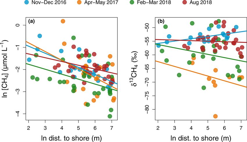
1334                 C. Soued and Y. T. Prairie: Changing sources and processes sustaining surface CO2 and CH4 fluxes

et al., 2017; Monteith et al., 2007). Soil-derived gas inputs       and the role of this process in fuelling surface GHG emis-
are also temporally variable, generally increasing with dis-        sions. The movement of gases within a system depends on
charge, like during storm events (Vachon and del Giorgio,           the structure of the water column, which changes spatially
2014) or rainy seasons (Kim et al., 2000; Zhang et al., 2019).      along the aquatic continuum. Reservoirs in particular exhibit
Terrestrial inputs in the form of organic C can indirectly sus-     strong gradients in morphometry and hydrology, translating
tain surface GHG emissions by fuelling lake and reservoir in        into high spatial heterogeneity in surface GHG fluxes to the
situ organic matter respiration (Karlsson et al., 2007; Pace        atmosphere (Paranaíba et al., 2018; Teodoru et al., 2011).
and Prairie, 2005; Rasilo et al., 2017).                               Understanding what regulates surface CO2 and CH4 con-
   The net internal balance between production and con-             centrations and fluxes to the atmosphere thus requires knowl-
sumption processes of CO2 and CH4 ultimately determines             edge of the interplay between all physical and biogeochem-
their surface fluxes. For CO2 , aerobic ecosystem respiration       ical processes involved and how they vary spatially. While
(ER) and gross primary production (GPP) are highly vari-            a number of studies have assessed some processes individ-
able in space and time and generally a function of tem-             ually or by difference, very few have measured all relevant
perature, organic C content, and nutrients (Hanson et al.,          components of the epilimnetic mass balance simultaneously.
2003; Pace and Prairie, 2005; Prairie et al., 1989; Solomon         Here we report on a field study in a tropical East Asian hy-
et al., 2013). Net heterotrophy (ER > GPP) is mainly associ-        dropower reservoir quantifying external inputs, sediment in-
ated with systems receiving high external inputs of organic         puts, net CO2 and CH4 metabolism, vertical diffusion from
C (Bogard et al., 2020; Tank et al., 2010; Wilkinson et al.,        deeper layers, and gas exchange at the air–water interface.
2016), while net autotrophy (ER < GPP) has been associated          This allowed us to estimate the relative contribution of each
with highly productive nutrient-rich systems (Hanson et al.,        process in shaping surface GHG emissions from the reser-
2003; Sand-Jensen and Staehr, 2009). However, a large part          voir and to test whether the epilimnetic mass balance can
of the variability in measured metabolic rates remains unex-        be closed. The two major rivers feeding the reservoir flow
plained (Bogard et al., 2020; Coloso et al., 2011; Solomon          into two elongated branches, acting as transition zones, be-
et al., 2013), impeding our ability to accurately predict their     fore reaching the main basin. This configuration, common in
net balance. Additionally, anaerobic C transformation adds          reservoirs, allowed us to quantify and compare epilimnetic
another level of complexity to the C metabolic balance by           CO2 and CH4 regulation in two morphometrically different
decoupling GPP and ER (Bogard and del Giorgio, 2016;                areas (reservoir branches and main basin). Overall, the aim
Martinsen et al., 2020; Vachon et al., 2020). For instance,         of this study is to provide an ecosystem-scale portrait of the
acetoclastic methanogenesis can transform organic C to CH4          processes sustaining surface CO2 and CH4 emissions and ex-
instead of CO2 , and hydrogenotrophic methanogenesis con-           amine how they change when transitioning from a river delta
verts CO2 to CH4 without producing O2 .                             to an open basin.
   For CH4 , production occurs in both profundal and littoral
sediments, and CH4 reaches the water surface by vertical or
lateral diffusive processes (Bastviken et al., 2008; DelSontro      2     Materials and methods
et al., 2018b; Encinas Fernández et al., 2014; Guérin et al.,
2016). However, there is increasing evidence that CH4 pro-          2.1    Site and sampling description
duction in the oxic water column can also contribute sig-
nificantly to lake CH4 emissions (Bižić et al., 2019; Bog-         The study was conducted in the Batang Ai hydroelectric
ard et al., 2014; DelSontro et al., 2018b; Donis et al., 2017;      reservoir in Sarawak, Malaysia (latitude 1.16◦ and longi-
Tang et al., 2014). Methanogenesis can be counter-balanced          tude 111.9◦ ). The reservoir is located in Borneo in a trop-
by the oxidation of CH4 to CO2 mainly in oxic and hypoxic           ical equatorial climate with a constantly high temperature
environments (Conrad, 2009; Reis et al., 2020; Thottathil           averaging 23 and 32 ◦ C during nighttime and daytime re-
et al., 2019). While several studies have measured rates of         spectively (Sarawak Government, 2019). The region expe-
CH4 production and oxidation in lakes and reservoirs, few           riences two weak monsoon seasons (November to Febru-
have quantified the net balance of these two processes at an        ary and June to October) with a yearly average rainfall of
ecosystem scale (Bastviken et al., 2008; Schmid et al., 2007),      3300 to 4600 mm (Sarawak Government, 2019). The reser-
a balance tightly linked to physical processes within the wa-       voir was impounded in 1985 with a dam wall of 85 m, a sur-
ter column (Vachon et al., 2019).                                   face area of ∼ 68.4 km2 , and a watershed area of 1149 km2
   For both gases, physical mixing in lakes and reservoirs in-      of mostly undisturbed forested land (limited rural habitations
directly impacts C metabolic processes by shaping the O2            and small-scale croplands).
profile and directly affects GHG surface diffusion by con-             We distinguish between three sections of the study site: in-
trolling the transport of CO2 and CH4 from deep to surface          flows, reservoir branches, and the reservoir main basin shown
water layers (Barrette and Laprise, 2005; Kreling et al., 2014;     in Fig. 1. The inflows are the two main reservoir inlets: the
Pu et al., 2020). Despite its potential importance (Kankaala        Batang Ai and Engkari rivers (3 to 10 m deep where sam-
et al., 2013), very few studies quantified vertical gas transport   pled). The two rivers flow into two arms that we refer to

Biogeosciences, 18, 1333–1350, 2021                                                   https://doi.org/10.5194/bg-18-1333-2021
C. Soued and Y. T. Prairie: Changing sources and processes sustaining surface CO2 and CH4 fluxes                                  1335

Figure 1. Map of Batang Ai reservoir with delimited sections (branches and main basin) and sampling points. ∗ Represents sampling points
at the branches’ extremities.

as the reservoir branches (10.8 km2 , mean and max depths             sured temperature profiles using the R package rLakeAna-
of 18 and 52 m respectively). The reservoir branches merge            lyzer (Winslow et al., 2018). The epilimnion was defined
into the main basin of the reservoir (58.9 km2 , mean and max         from the surface to the top of the metalimnion and was as-
depths of 30 and 73 m respectively). Surface sampling was             sumed to be a mixed layer.
performed at 36 sites across the three study sections, and
water column profile sampling (from 0 up to 32 m, each 0.5            2.3   Gas concentration, isotopic signature, and
to 3 m) was done at nine sites in the reservoir branches and                water–air fluxes
main basin (Fig. 1). Sampling was repeated (with a few ex-
ceptions) during four campaigns: (1) 14 November to 5 De-             CO2 and CH4 gas concentrations and isotopic signatures
cember 2016 (November–December 2016), (2) 19 April to                 (δ 13 C) were measured in duplicates at the surface at 36 sites
3 May 2017 (April–May 2017), (3) 28 February to 13 March              and along vertical profiles at nine sites (P1 to P9, Fig. 1) us-
2018 (February–March 2018), and (4) 12 to 29 August 2018              ing the headspace technique described in detail in Soued and
(August 2018).                                                        Prairie (2020). In brief, sampling was done by equilibrating
                                                                      the water sample for 2 min with an air headspace inside a
2.2   Physical and chemical analyses                                  60 mL syringe. The gas phase was then injected in a 12 mL
                                                                      pre-vacuumed airtight vial and analyzed on a gas chromato-
Water temperature, dissolved oxygen, and pH were mea-                 graph (Shimadzu GC-8A with a flame ionization detector)
sured using a multi-parameter probe (YSI model 600XLM-                for gas concentrations and on a cavity ring-down spectrom-
M) equipped with a depth gauge and attached to a 12 V                 eter (CRDS) equipped with a small sample isotopic module
submersible pump (Proactive Environmental Products model              (SSIM, Picarro G2201-i) for δ 13 CO2 and δ 13 CH4 .
Tornado) for water sample collection. Concentrations of dis-              Surface gas flux data used in this study are described in
solved organic carbon (DOC), total phosphorus (TP), total             more detail in Soued and Prairie (2020), a previous study
nitrogen (TN), and chlorophyll a (chl a) were measured                on the C footprint of Batang Ai reservoir. Surface diffu-
during all campaigns at all surface sampling sites (Fig. 1).          sive fluxes of CO2 and CH4 were measured at all surface
Methods for these analyses are described in detail in Soued           sampling sites during each campaign. Flux rates were de-
and Prairie (2020). Briefly, TP and chl a (extracted with             rived from linear changes in CO2 and CH4 concentrations
hot ethanol) were analyzed via spectrophotometry, and TN              in a static floating chamber (design described in Soued and
and DOC (filtered at 0.45 µm) were measured on an Alpkem              Prairie, 2020 and IHA, 2010) connected in a closed loop to
Flow Solution IV autoanalyzer and on a total organic carbon           a portable gas analyzer (model UGGA, from Los Gatos Re-
analyzer 1010-OI respectively.                                        search). Measured gas concentrations, isotopic signature, and
   For each site, we defined the depths of the thermocline            fluxes were spatially interpolated to the whole reservoir area
and the top and bottom of the metalimnion based on mea-               by inverse distance weighting (given the absence of a suitable

https://doi.org/10.5194/bg-18-1333-2021                                                       Biogeosciences, 18, 1333–1350, 2021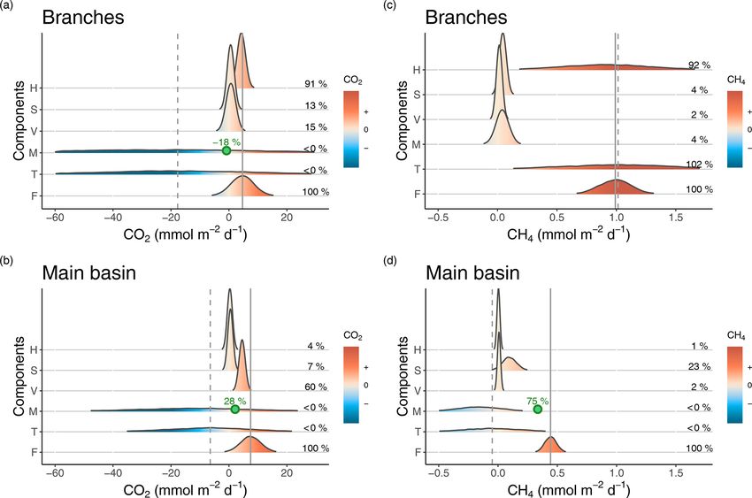
1336                 C. Soued and Y. T. Prairie: Changing sources and processes sustaining surface CO2 and CH4 fluxes

variogram for kriging) using package gstat version 1.1-6 in        derived from the following Eq. (3) (Osborn, 1980):
the R version 3.4.1 software (Pebesma, 2004). Mean values

were calculated for each campaign based on the interpolated        Kz = 0      ,                                               (3)
maps (Soued and Prairie, 2020).                                             N2
                                                                   where 0 is the mixing ratio set to 0.2 (Oakey, 1982),  is
2.4    Horizontal GHG inputs
                                                                   the dissipation rate of turbulent kinetic energy, and N 2 is
In order to estimate the external horizontal inputs of CO2         the buoyancy frequency. N 2 was calculated from measured
and CH4 , we considered that the total volume of water in-         temperature profiles (YSI probe) using the function buoy-
flow and outflow (discharge measured at the dam) were equal        ancy.freq from the rLakeAnalyzer package (Winslow et al.,
and equivalent to the mean of measured daily discharge             2018) in the R software (R Core Team, 2017).  was de-
(Q, in m3 d−1 ) during each campaign (considering minimal          rived from measured vertical shear microstructure profiles
changes in inflow and outflow rates during a campaign). The        performed in the August 2018 campaign at all profile sites
approach of using discharge as a measure of total water in-        shown in Fig. 1 (except P1 due to floating logs). Shear pro-
flow has the advantage of integrating all external flow (rivers,   files were measured with a high-frequency (512 Hz) Mi-
lateral soils, and groundwater) as water inputs to the reser-      croCTD profiler (Rockland Scientific) equipped with two ve-
voir. However, the fraction of inflow feeding the reservoir        locity shear probes, two thermistors, tilt and vibration sen-
surface vs. bottom layer and its average gas concentration can     sors, and a pressure sensor. At each site, the profiler was cast
only be approximated based on measurements from the two            10 times, five with an uprising configuration (from bottom to
main river inlets (Fig. 1) due to the lack of data on other lat-   top of the water column) and five with a downward config-
eral inflows. Given that part of the inflowing water is colder     uration (top to bottom), with a 4 min waiting time between
and denser than the reservoir surface layer, only a fraction       profiles to allow water column disturbance to subside. Data
of it enters the epilimnion of the reservoir branches, and the     quality check and  calculation for each profile cast were per-
rest plunges into the hypolimnion. We estimated that fraction      formed with the ODAS v4.3.03 MATLAB library (developed
(fepi ) based on temperature profiles in the eastern river delta   by Rockland Scientific) based on Nasmyth shear spectrum
and branch (sites P1 and P2, Fig. 1), and we assumed it is rep-    (Oakey, 1982), with  values averaged among the two shear
resentative of other water inflows to the reservoir. The areal     probes and binned over 1–2 m segments along the profile. For
rate of horizontal CO2 and CH4 inputs (H , in mmol m−2 d−1 )       each site, continuous  profiles were interpolated by fitting a
over each section of the reservoir were then calculated fol-       smooth spline through all  values from replicate casts as a
lowing Eq. (1):                                                    function of depth.
                                                                      At the epilimnion–metalimnion interface (top of the metal-
       Cin Qfepi                                                   imnion ±2 m), calculated  averaged 7.7 × 10⁻⁹ (range from
H=               ,                                          (1)
           A                                                       3.4×10⁻⁹ to 1.6×10⁻⁸ ) m2 s−3 across all sites sampled with
                                                                   the MicroCTD, with no significant difference between the
with A (m2 ) the surface area of the reservoir section consid-     main basin and branch sites. In order to estimate vertical gas
ered and Cin (mmol m−3 ) the concentration of gas in the in-       diffusion, we applied the latter  average to Eqs. (2) and (3)
flowing water. To estimate gas inputs from the inflows to the      for all measured gas profiles (except P1). The resulting V val-
branches, Cin was considered to be the average of gas con-         ues for each gas were averaged across sites in the main basin
centrations measured at the two upstream extremities of the        and branches separately to derive estimates of V for each of
branches (Fig. 1). To estimate gas inputs from the branches to     these two reservoir sections.
the main basin, Cin was considered to be the gas concentra-
tions measured at the confluence between the two branches          2.6   Sediment GHG inputs
(right upstream of the main basin).
                                                                   We calculated CO2 and CH4 inputs from the sediments
2.5    Vertical GHG fluxes                                         to epilimnetic waters using gas profiles in sediment cores
                                                                   collected in April–May 2017 and February–March 2018 at
We estimated CO2 and CH4 fluxes from the metalimnion
                                                                   seven sites (P1 to P3 in the reservoir branches and P4, P5,
to the epilimnion (V ) based on the vertical gas diffusiv-
                                                                   P7, and P9 in the main basin, Fig. 1). Sediment cores were
ity (Kz ) and the gradient in gas concentration across the
                                                                   collected using a Glew gravity corer attached to a 6 cm wide
epilimnion–metalimnion interface using Eq. (2) (Wüest and
                                                                   plastic liner. The liner was predrilled with 1 cm holes cov-
Lorke, 2009):
                                                                   ered with electric tape at each centimetre up to 40 cm. Upon
V = Kz (Cmeta − Cepi ),                                     (2)    recovery of the sediment core, 3 mL tip-less syringes were in-
                                                                   serted into each hole to extract sediments from each centime-
where Cmeta and Cepi are the gas concentrations at the top of      tre. The sediment content of each syringe was emptied into a
the metalimnion and at the bottom of the epilimnion respec-        25 mL glass vial prefilled with 6 mL nano-pure water and im-
tively, measured at profile sites (P1 to P9, Fig. 1). Kz was       mediately airtight sealed by a butyl rubber stopper crimped

Biogeosciences, 18, 1333–1350, 2021                                                   https://doi.org/10.5194/bg-18-1333-2021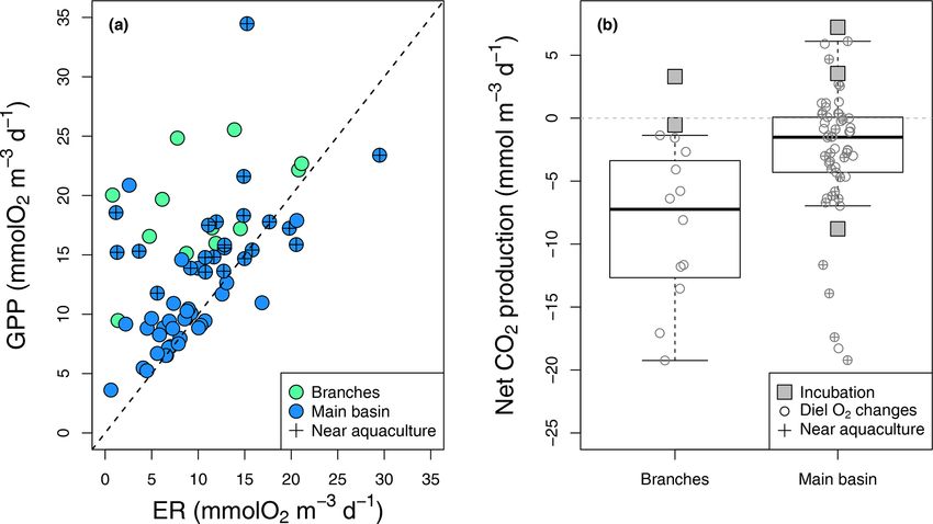
C. Soued and Y. T. Prairie: Changing sources and processes sustaining surface CO2 and CH4 fluxes                              1337

with an aluminum cap. Glass vials were pressurized with            (Soued and Prairie, 2020). Therefore, sediment ebullition
40 mL of ambient air using a plastic syringe equipped with         was considered negligible in the epilimnetic CH4 budget of
a needle to pierce the rubber cap. Glass vials were shaken         Batang Ai.
for 2 min for equilibration before extracting the gas with a
syringe and injecting it into a pre-evacuated airtight vial for    2.7   Metabolic rates
analysis of CO2 and CH4 concentrations and isotopic signa-
tures as described above. Additionally, samples of the water       Net metabolic rates of CO2 and CH4 production in the epil-
overlaying the sediments (∼ 1 cm above) were collected for         imnetic water column were estimated with in situ incuba-
similar analyses of CO2 and CH4 .                                  tions. Incubations were performed at five sites (P2 and P3 in
   Sediment CO2 and CH4 flux rates to the overlaying wa-           the branches and P4, P5, and P7 in the main basin, Fig. 1).
ter column were derived from the vertical gradient of gas          Water from 3 m deep was pumped into 5 L transparent glass
concentration measured in the sediment cores and overlaying        jars with an airtight clamp lid. Before closing, jars were filled
water. The slope of CO2 or CH4 concentration as a function         from the bottom and allowed to overflow and then sampled
of depth (g, in µmol L−1 m−1 ) was calculated for measured         for initial CO2 and CH4 concentrations. Closed jars were
values in the first 5 cm of sediments and overlaying water.        fixed at 3 m to an anchored line at the sampling site and incu-
Most cores exhibited clear linear slopes (p value < 0.05 and       bated in in situ temperature and light conditions for 22.0 to
  2 > 0.5). In the few cases where a linear slope was not ev-
Radj                                                               24.2 h. Upon retrieval, samples of final CO2 and CH4 con-
ident, g was replaced by the gradient between the mean gas         centrations were collected from the jars. Volumetric daily
concentration in the first 3 cm of sediments and the overlay-      rates of net CO2 and CH4 production were calculated based
ing water. The sediment gas flux rate (Sf in mmol m−2 d−1 )        on the difference between final and initial gas concentrations
was calculated with Eq. (4):                                       rescaled to a 24 h period.
                                                                      In addition to incubations, open-water high-frequency O2
       g×d                                                         measurements were carried out to derive CO2 metabolism on
Sf =       ,                                                (4)
        p                                                          larger spatial and temporal scales. Rates of GPP, ER, and net
                                                                   ecosystem production (NEP) were estimated in the reservoir
with d the diffusion coefficient set to 1.5×10⁻⁵ cm2 s−1 (Do-
                                                                   surface layer by monitoring and inverse modelling diel O2
nis et al., 2017) and p the sediment porosity assumed to be
                                                                   changes in the epilimnion. O2 was measured at a 1 min inter-
2 % based on previous results in Batang Ai (Tan, 2015).
                                                                   val using high-frequency O2 and temperature sensors (model
   At an ecosystem scale, sediment CO2 and CH4 inputs to
                                                                   miniDOT from Precision Measurement Engineering), along
the water column (S) were estimated based on average and
                                                                   with light sensors (model HOBO Pendant from Onset). Sen-
standard deviation values of sites located in each section of
                                                                   sors were deployed in profile sites P1 to P3 in the branches
the reservoir (branches and main basin). For each section,
                                                                   and P4, P5, P7, and P9 in the main basin (Fig. 1). Note that
mean sediment CO2 and CH4 flux rates were multiplied by
                                                                   not all sites were sampled in all sampling campaigns. Sen-
the areal ratio of epilimnetic sediments (Aepi ) vs. total water
                                                                   sors were attached to an anchored line at a depth between
area (A0 ). The latter ratio was calculated based on the hypso-
                                                                   0.7 and 3 m and deployment time varied between 4 d and 2
metric model (Ferland et al., 2014; Imboden, 1973) as shown
                                                                   weeks. Upon retrieval of the sensors, the first data quality
in Eqs. (5) to (7):
                                                                   check and selection were made based on the sensor inter-
                                                                   nal quality index and visual screening. Rates of ecosystem

        zmax
q=               − 1,                                        (5)   metabolism were then estimated based on an open-system
       zmean
                             q                               diel O2 model (Odum, 1956), where change in O2 concen-
                           zepi
Aepi = A0 1 − 1 −                     ,                      (6)   tration is a function of GPP, ER, and air–water gas exchange
                           zmax                                    (KO2 ) following Eq. (8) (Hall and Hotchkiss, 2017):
     Aepi
S=         Sf ,                                              (7)   dO2   GPP ER
      A0                                                               =      +      + KO2 (O2sat − O2 ) ,                      (8)
                                                                    dt   zepi   zepi
with q a parameter describing the general bathymetric shape
of the reservoir section, zmax and zmean the maximum and           with O2sat the theoretical O2 concentration at saturation con-
mean depths respectively, and zepi the mean depth of the           sidering the in situ temperature and atmospheric pressure,
epilimnion (8.0 and 10.5 m in the branches and main basin          and O2 is the actual measured O2 concentration in the water.
respectively).                                                     A detailed description of the model equations can be found
   Littoral sediments are known to be a source of CH4 not          in Hall and Hotchkiss (2017). Daily estimates of GPP, ER,
only through diffusion but also via ebullition. While this         and K600 (based on KO2 ) were derived by maximum likeli-
emission pathway was found to be important in other reser-         hood fitting of the data to the model in Eq. (8) using the R
voirs (Deemer et al., 2016), it is surprisingly low in Batang      package StreamMetabolizer (Appling et al., 2018). Note that
Ai, equaling less than 2 % of CH4 surface diffusive emis-          even though the package used was originally developed for
sions, and only 0.1 % of the reservoir total GHG footprint         streams, it is easily transferable to lakes given that the model

https://doi.org/10.5194/bg-18-1333-2021                                                    Biogeosciences, 18, 1333–1350, 2021
1338 C. Soued and Y. T. Prairie: Changing sources and processes sustaining surface CO2 and CH4 fluxes
used (Eq. 8) is generalized for all water bodies, with the pa-
rameter zepi describing the depth of a mixed water column
of either a lentic or lotic system and with the K600 estimate
relying only on data fitting to the model and not on system
type. In some cases, where the best predicted K600 was neg-
ative, the fitting process was rerun with a user-defined posi-
tive K600 , either equal to a value estimated for the previous
or subsequent day at the same site (range of 0.03–0.96 d−1 )
or fixed to 0.1 d−1 (if there is no other available estimate).
When considering the epilimnion depth, predicted values of
K600 translate into a first to third quantile range of 1.17 to
5.55 m d−1 , which is similar to the range of K600 values back-
calculated from surface gas flux measurements with the float-
ing chamber technique. A final selection of daily metabolic
estimates was done based on the model goodness of fit as-
sessed by calculating Pearson correlation coefficient between
modelled and measured O2 values and discarding days with a
correlation lower than 0.9. Based on GPP and ER estimates,
we calculated daily NEP as the balance between these two
processes, and we converted it to net CO2 production rate by
assuming an O2 : CO2 metabolic quotient of 1.
Areal metabolic rates were derived by integrating volu-
metric rates over the depth of the epilimnion. Average es- Figure 2. Average of spatially interpolated surface CO2 (a–c) and
CH4 (d–f) fluxes (a, d), concentrations (b, e), and isotopic signa-
timates of areal metabolic rates per campaign were obtained
tures (c, f) along the hydrological continuum from the reservoir in-
for the branches and main basin by first averaging data within
flows to the main basin for each sampling campaign.
each site and then across sites for each reservoir section. Note
that one value derived from incubations was excluded from
the calculation of the average net CH4 production rate in the 3 Results
branches due to its high value of initial CH4 concentration
(an order of magnitude higher than in all other incubations 3.1 Physical and chemical properties
and all epilimnetic data from this site). The high CH4 con-
centration, unrepresentative of real conditions, was probably Surface water temperature exhibited a marked increase from
caused by CH4 contamination during sampling and triggered the inflows to the branches, averaging 27.1 and 30.7 ◦ C re-
a high oxidation rate that would overestimate the real ecosys- spectively (Table 1). There was no difference in surface water
tem average rate if included. temperature between the branches and the main basin. The
depth of the epilimnion tended to increase and become more
stable along the water flow, going from 1.3 (±1.6) m in the
2.8 Epilimnetic GHG budgets Batang Ai River delta to 8.0 (±2.3) m in its branch and 10.6
(±1.7) m in the main basin (Table 1). Light penetration ex-
hibited the same spatial pattern, with an increasing Secchi
Areal rates of horizontal, vertical, sediment, and metabolic depth along the water flow averaging 1.3, 5.1, and 5.5 m in
inputs were combined into a sum of sources and sinks and the inflows, branches, and main basin respectively (Table 1).
compared to the rate of surface gas flux for each gas in each All sections of the study system exhibited oligotrophic water
reservoir section. A mean and standard error were calcu- properties (Table 1).
lated for every component of the budgets based on measure-
ments averaged across sites and/or sampling campaigns in 3.2 Surface GHG concentrations, fluxes, and isotopic
order to obtain ecosystem-scale estimates of the component signatures
means and uncertainties. In the case of CO2 metabolism, the
ecosystem-scale average was calculated as the mean of the Surface CO2 and CH4 patterns are summarized in Fig. 2,
two average values derived from the incubation and diel O2 presenting campaign averages of spatially interpolated gas
monitoring methods. For every component, density curves concentration, flux, and isotopic signature along the different
were derived considering a normal distribution based on the reservoir sections. Despite the temporal variability, the gas
mean and its standard error in order to visualize the relative patterns along the water flow are robust, remaining similar
magnitude and uncertainty of each ecosystem-scale areal rate throughout time (Fig. 2).
(Fig. 3).
Biogeosciences, 18, 1333–1350, 2021 https://doi.org/10.5194/bg-18-1333-2021C. Soued and Y. T. Prairie: Changing sources and processes sustaining surface CO2 and CH4 fluxes 1339
Table 1. Mean (±SD) of physical and chemical variables measured at the surface of the three reservoir sections.
Variables Units Inflows Branches Main basin
zepi m 1.3 (±1.6) 8 (±2.3) 10.6 (±1.7)
Secchi m 1.2 (±0.9) 5.1 (±1.2) 5.5 (±1.2)
Temperature ◦C 27.1 (±2.5) 30.7 (±0.5) 30.6 (±0.5)
pH 6.5 (±0.3) 7.2 (±0.2) 7.2 (±0.2)
O2 % 94.9 (±7.7) 102.7 (±4.5) 99.3 (±4.8)
DOC mg L−1 0.8 (±0.4) 0.9 (±0.2) 0.9 (±0.2)
TP µg L−1 20.7 (±7.6) 6.2 (±1.7) 5.8 (±2.6)
TN mg L−1 0.14 (±0.04) 0.12 (±0.04) 0.1 (±0.03)
Chl a µg L−1 2.1 (±1.7) 1.7 (±1) 1.2 (±0.5)
Average CO2 air–water flux and surface concentra- 3.3 Horizontal GHG flow
tion were systematically higher in the inflows (mean
[range]: 135.3 [18.9–368.8] mmol m−2 d−1 and 58.0 [24.5– Horizontal inputs from the inflows to the surface layer of the
113.0] µmol L−1 respectively) compared to the branches (4.7 branches were estimated to vary between 0.34–0.71 mol s−1
[−3.4–15.2] mmol m−2 d−1 and 15.4 [12.2–19.3] µmol L−1 ) for CO2 and 0.02–0.25 mol s−1 for CH4 . When expressed as
and main basin (7.5 [0.3–15.1] mmol m−2 d−1 and 16.0 areal rates over the branches (to facilitate comparison with
[14.2–17.7] µmol L−1 ) (Fig. 2a and b). Surface CO2 con- other components), horizontal inputs amounted to 2.7–5.7
centration in the reservoir (branches and main basin) was and 0.16–1.97 mmol m−2 d−1 for CO2 and CH4 respectively
most strongly correlated inversely with water temperature (Tables S2 and S3 in the Supplement). These values are of
2 = 0.22, p value < 0.001, Fig. S1a and Table S1 in the
(Radj the same order of magnitude as surface fluxes calculated in
Supplement). Except for the April–March 2017 campaign, the branches (Fig. 3a and c, Tables S2 and S3). However, the
there was a modest increase (2.2 ‰ to 3.3 ‰) in surface effect of horizontal inputs faded spatially, with much lower
δ 13 CO2 towards more enriched values from the inflows to inputs from the branches to the main reservoir basin, aver-
the branches (Fig. 2c). aging 0.31 and 0.004 mmol m−2 d−1 for CO2 and CH4 re-
Similarly, surface CH4 flux and concentration continually spectively (Fig. 3b and d and Tables S2 and S3). For CH4 ,
decreased along the water channel, being an order of mag- this fits spatial and temporal surface flux measurements, be-
nitude higher in the inflows compared to the branches and ing systematically higher in the branches and maximal dur-
about twice as high in the branches compared to the main ing the two sampling campaigns with the highest recorded
basin (Fig. 2d and e). Of all measured water properties, TN horizontal inputs from the inflows (Table S3). In contrast,
was the most strongly linked to reservoir surface CH4 con- CO2 surface flux was typically lower (sometimes negative)
2 = 0.14, p value < 0.001, Fig. S1b and Ta-
centration (Radj in the branches compared to the main basin, despite substan-
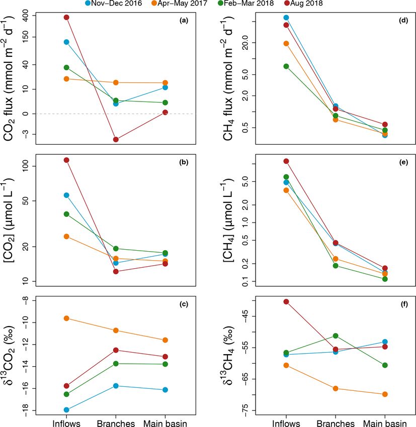
ble S1). In the main basin, surface CH4 concentration sig- tial riverine inputs to the branches (Table S2).
nificantly decreased with distance to shore in November–
December 2016 (Radj 2 = 0.54, p value < 0.001), but this cor- 3.4 Vertical GHG inputs
relation was weaker (Radj2 ≤ 0.13, p value ≥ 0.03) during
Vertical fluxes depend on the gas diffusivity and concentra-
other sampling campaigns (Fig. 6a). Surface δ 13 CH4 val- tion gradient. Gas diffusivity is a function of the strength
ues varied widely, between −83.3 and −47.6 ‰, but did of stratification (N 2 ) and energy dissipation rate (). Mea-
not show a consistent spatial pattern (Fig. 2f) apart from a sured values of N 2 and varied widely, from 5.9 × 10⁻⁵ to
positive correlation with distance to shore in the main basin 2.3 × 10⁻³ s−2 and from 3.4 × 10⁻⁹ to 1.6 × 10⁻⁸ m2 s−3 re-
in November–December 2016 (Radj 2 = 0.29, p value = 0.01,
spectively, but with no clear differences between the reser-
Fig. 6b). voir branches and main basin (Fig. S3a and b in the Sup-
The degree of coupling between CO2 and CH4 followed plement). Similarly, CO2 and CH4 concentration gradients
a clear spatial pattern. While CO2 and CH4 surface con- varied substantially in both space and time (from −18.4 to
2 = 0.54,
centrations were strongly linked in the inflows (Radj 94.3 µmol L−1 m−1 for CO2 and −0.19 to 0.4 µmol L−1 m−1
p value = 0.006), they became only weakly correlated in the for CH4 ). CO2 concentration generally increased from the
2 = 0.17, p = 0.005) and not correlated at all in
branches (Radj epilimnion to the metalimnion as a result of the respiratory
2 = 0.01, p value = 0.11) (Fig. S2 in the
the main basin (Radj CO2 buildup in the deep layer. On rare occasions, an inverse
Supplement). gradient was observed, possibly due to autotrophic activ-
ity in the metalimnion. For CH4 , metalimnion-to-epilimnion
concentration gradients were generally modest, averaging
https://doi.org/10.5194/bg-18-1333-2021 Biogeosciences, 18, 1333–1350, 20211340 C. Soued and Y. T. Prairie: Changing sources and processes sustaining surface CO2 and CH4 fluxes
Figure 3. Density distributions of the different components of CO2 (a, b) and CH4 (c, d) surface budgets in the reservoir branches (a, c)
and main basin (b, d). Components are as follows. H : horizontal flow inputs; S: sediment inputs; V : vertical inputs; M: net metabolism
(average of the incubation and diel O2 monitoring methods); T : sum of all estimated sources and processes in the surface layer; F : measured
surface fluxes. Density curves are based on simulated normal distributions using the mean and standard error of each component. The x axes
represent the areal rate of CO2 or CH4 , and the colour scale indicates the sign of the rate. Mean values of the fraction of each component
(%) relative to the mean surface flux (F ) are reported on the right side in each panel. The solid and dashed grey lines represent the means of
F and T respectively. In panels (a), (b), and (d), the point and percentage in green represent the hypothetical value of the M rate (the most
uncertain component) and its corresponding fraction (as a percentage of F ) that are needed to close the budget (to obtain T = F ).
0.04 µmol L−1 m−1 , and even negative in one-third of the ments in each section yields estimates of sediment inputs to
profiles, leading to the diffusion of epilimnetic CH4 to- the epilimnion of 0.6 (±0.03) and 0.5 (±0.11) mmol m−2 d−1
ward deeper layers instead of the reverse. The low to nega- for CO2 and 0.04 (±0.02) and 0.10 (±0.06) mmol m−2 d−1
tive CH4 vertical flux results from a highly active methan- for CH4 in the branches and main basin respectively (Fig. 3
otrophic layer reducing CH4 concentration in the metal- and Tables S2 and S3). These inputs from littoral sediments
imnion, as evidenced by the strong enrichment effect ob- likely represent an upper limit since they are based on deep
served in δ 13 CH4 profiles (Fig. S4 in the Supplement). pelagic sediment cores (littoral area were too compact for
The combination of vertical diffusivity and gas concen- coring), where a higher organic matter accumulation and
tration gradients resulted in vertical fluxes averaging 3.4 degradation is expected (Blais and Kalff, 1995; Soued and
(−1.8 to 20.5) mmol m−2 d−1 for CO2 and 0.01 (−0.01 to Prairie, 2020). Even as upper estimates, the calculated rates
0.09) mmol m−2 d−1 for CH4 , with no significant differences of sediment GHG inputs remain a relatively modest fraction
between the reservoir branches and main basin (Fig. S3). of the average emissions to the atmosphere for the branches
and main basin for both CO2 (13 % and 7 % respectively) and
3.5 GHG inputs from littoral sediments CH4 (4 % and 23 % respectively) (Tables S2 and S3).
Areal sediment gas fluxes ranged from 1.2 to 4.0 and −0.29 3.6 Metabolism
to 1.10 mmol m−2 d−1 for CO2 and CH4 respectively (Fig. S5
in the Supplement), in the range of previously reported values 3.6.1 CO2 metabolism
in lakes and reservoirs (Adams, 2005; Algesten et al., 2005;
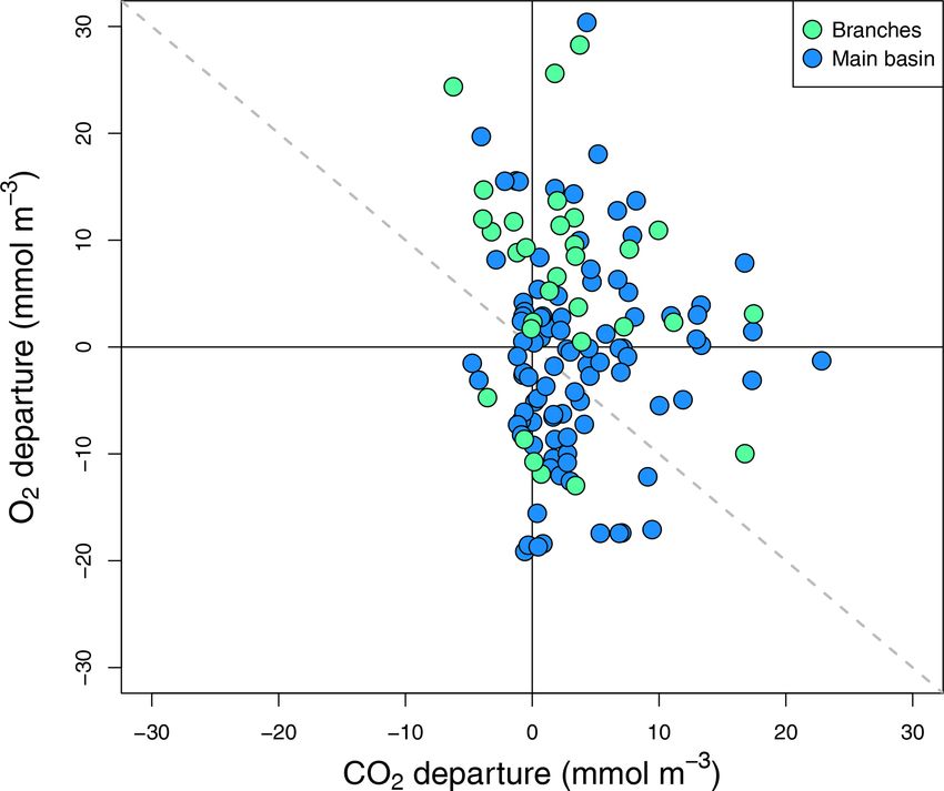
Gruca-Rokosz and Tomaszek, 2015; Huttunen et al., 2006). Estimated GPP and ER rates based on diel O2 monitor-
Sediment fluxes were not different in the branches vs. the ing ranged from 3.6 to 34.5 µmol L−1 d−1 and from 5.8
main basin for both CO2 (mean of 2.2 vs. 2.4 mmol m−2 d−1 ) to 29.5 µmol L−1 d−1 respectively (Fig. 4a), which is well
and CH4 (mean of 0.17 vs. 0.48 mmol m−2 d−1 ) (Fig. S5). within the range of reported rates for oligotrophic systems
Applying measured averages to the area of epilimnetic sedi- (Bogard and del Giorgio, 2016; Hanson et al., 2003; Solomon
Biogeosciences, 18, 1333–1350, 2021 https://doi.org/10.5194/bg-18-1333-2021C. Soued and Y. T. Prairie: Changing sources and processes sustaining surface CO2 and CH4 fluxes 1341
Figure 4. Epilimnetic daily GPP vs. ER rates (a) derived from diel O2 changes in the reservoir branches and main basin (including sites near
aquacultures), with the 1 : 1 line (dotted). (b) Boxplots of the corresponding rates of CO2 NEP in the branches and main basin, with box
bounds, whiskers, solid line, open circles, and squares representing the 25th and 75th percentiles, the 10th and 90th percentiles, the median,
single data points (diel O2 method), and incubation-derived rates respectively.
Figure 6. Regression of CH4 concentration (a) and isotopic sig-
nature (b) as a function of distance to shore in each sampling
campaign in the main reservoir basin. For CH4 concentration, re-
gressions lines have the following statistics in order of sampling:
p values: < 0.001, 0.06, 0.03, and 0.05 and Radj2 : 0.54, 0.13, and
Figure 5. Surface O2 vs. CO2 departure from saturation for all sam-
0.11. For δ 13 CH4 , all regressions had p values > 0.2 except for
pled surface sites in the reservoir main basin and branches across all
the November–December 2016 campaign with a p value = 0.01 and
sampling campaigns. 2 = 0.29.
Radj
et al., 2013). As expected, GPP and ER rates were corre-
2 = 0.23, p value < 0.001, Fig. 4a), with photosyn-
lated (Radj In the reservoir branches, results from the diel O2 mon-
thesis stimulating the respiration of produced organic matter. itoring method suggested systematic net CO2 uptake rang-
In most cases, GPP exceeded ER, especially in the branches ing from −19.2 to −1.4 µmol L−1 d−1 , whereas results from
and near aquacultures (Fig. 4a), where higher nutrients (TP two incubations were slightly above that range (−0.5 to
and TN) and chl a concentrations were measured (Table 1). 3.3 µmol L−1 d−1 ) (Fig. 4b). In the main basin, incubation
Daily metabolic rates showed no correlation with mean daily results ranged from −8.8 to 7.2 µmol L−1 d−1 , while the
rain or light (Kendall rank correlation p value > 0.1). diel O2 technique captured a wider variability in net CO2
metabolic rates from −19.2 to 6.1 µmol L−1 d−1 , with an
estimated CO2 uptake in 39 out of 54 cases (Fig. 4b).
Areal net CO2 metabolic rates, as the average of the two
https://doi.org/10.5194/bg-18-1333-2021 Biogeosciences, 18, 1333–1350, 20211342 C. Soued and Y. T. Prairie: Changing sources and processes sustaining surface CO2 and CH4 fluxes
methods, yielded an ecosystem-scale estimate of −23.2 and ingly variable (switching from negative to positive NEP on
−11.8 mmol m−2 d−1 in the reservoir branches and main a daily timescale), thus making it difficult to derive a suf-
basin respectively (Table S2). ficiently precise ecosystem-scale estimate to close the epil-
To complement the metabolic rate data, surface O2 and imnetic budget (Fig. 3a and b), despite high sampling resolu-
CO2 departure from saturation was examined in both reser- tion (n = 66 daily metabolic rates). Including the metabolism
voir sections. O2 oversaturation was observed in 44 % of substantially shifts the mean of the CO2 epilimnetic budget
cases in the main basin and 81 % in the branches (Fig. 5), (sum of sources and sinks) to a negative value and drasti-
which corresponds with the spatial patterns of net metabolic cally increases its uncertainty (Fig. 3a and b and Table S2),
rates (Fig. 4b). CO2 oversaturation was also widespread reflecting a potentially important but poorly resolved role of
(74 % of cases), making many sampled sites oversaturated metabolism in the budget because of its variability. However,
in both O2 and CO2 (55 % in the branches and 32 % in the given that metabolism acts more likely as a CO2 sink on aver-
main basin, Fig. 5). age, our best assessment suggests that vertical transport from
deeper layers is the main source sustaining surface CO2 out-
3.6.2 CH4 metabolism flux in the main basin of Batang Ai.
Net metabolic CH4 rates (from incubations) ranged from 3.7.2 CH4 budget
−0.026 to 0.078 µmol L−1 d−1 , indicating that the CH4 bal-
ance in the epilimnion of Batang Ai varied from net oxida- In contrast with CO2 , vertical transport was the smallest
tion to net production (Table S3). CH4 metabolic rates mea- source of CH4 to the epilimnion, contributing to only 2 %
sured in Batang Ai are within the range of values observed of surface fluxes in both reservoir sections (Fig. 3c and d
in other systems for oxidation (Guérin and Abril, 2007; Thot- and Table S3). In the branches, sediment inputs and net CH4
tathil et al., 2019) and production (Bogard et al., 2014; Donis metabolic rates were both relatively low (mean of 0.04±0.02
et al., 2017). No temporal or spatial (branches vs. main basin) and 0.04 ± 0.05 mmol m−2 d−1 ) and had little impact on the
differences in net metabolic CH4 rate were detected due to a budget, corresponding each to 4 % of surface fluxes in that
high variability and limited data points. section (Fig. 3c and Table S3). On the other hand, horizon-
tal inputs were the dominant and most variable source sus-
3.7 Ecosystem-scale GHG budgets taining CH4 emissions in the branches, where the epilim-
netic mass balance closed almost perfectly (Fig. 3c and Ta-
Estimated sources and sinks of CO2 and CH4 were collated
ble S3). Despite being the main CH4 source in the branches,
into a budget to evaluate their relative impact on epilimnetic
horizontal transport was a negligible component in the main
gas concentration and to assess whether their sum matches
basin (1 % of the flux, Fig. 3d and Table S3). Instead, sed-
the measured surface gas fluxes in each section of the reser-
iment inputs played a larger role in that section, with a
voir. Figure 3 depicts such reconstruction of the epilimnetic
mean of 0.10 (±0.06) mmol m−2 d−1 , fuelling 23 % of sur-
CO2 and CH4 budgets in Batang Ai as well as the uncertainty
face emissions in the main basin (Fig. 3d and Table S3). As
limits of each component. While each process varied in time,
with CO2 , the most variable CH4 component of the mass
their relative importance in driving surface fluxes was gen-
balance in the main basin was the net metabolism within
erally similar from one sampling campaign to another (Ta-
the epilimnion (mean of −0.16 ± 0.19 mmol m−2 d−1 ). Con-
bles S2 and S3).
sidering all sources, the CH4 budget indicates a deficit of
3.7.1 CO2 budget 0.34 mmol m−2 d−1 to explain measured surface emissions
in the main basin (Fig. 3d and Table S3).
For CO2 , epilimnetic sediment inputs had a small contri-
bution, being typically an order of magnitude lower than
measured surface fluxes in both sections of the reservoir 4 Discussion
(Fig. 3a and b and Table S2). Vertical CO2 inputs from lower
depths on the other hand contributed substantially to sur- Our results have highlighted both the importance and the
face fluxes in the branches and especially in the main basin challenges associated with simultaneously quantifying all the
(mean of 0.7 and 4.5 mmol m−2 d−1 respectively, Fig. 3a and components of the epilimnetic CO2 and CH4 budgets, partic-
b and Table S2), indicating that hypolimnetic processes im- ularly in a hydrologically complex reservoir system. While
pact surface emissions despite the permanent stratification. mass fluxes (hydrological, sedimentary, and air–water fluxes)
Horizontal inputs of CO2 averaged 4.3 mmol m−2 d−1 in the are relatively easy to constrain, internal C processing, namely
branches; however, they decreased by an order of magnitude the net metabolic balances between production and con-
when reaching the main basin (mean of 0.3 mmol m−2 d−1 ). sumption of CO2 and CH4 , is highly dynamic in both time
Thus, direct CO2 inputs from the inflows notably increase and space, leading to significant uncertainties when extrapo-
surface flux rates in the reservoir branches but only mini- lated to the ecosystem scale. In many studies, some compo-
mally in the main basin. Net CO2 metabolism was surpris- nents are only inferred by difference. While convenient from
Biogeosciences, 18, 1333–1350, 2021 https://doi.org/10.5194/bg-18-1333-2021C. Soued and Y. T. Prairie: Changing sources and processes sustaining surface CO2 and CH4 fluxes 1343
a mass balance perspective, we argue that assessing all com- 2019; Gebert et al., 2006; Isidorova et al., 2019) and in the
ponents together is necessary to clearly identify knowledge oxic water column (Bogard et al., 2014), through its link with
gaps as well as sources of uncertainty. algal production and decomposition. However, CH4 concen-
tration and flux variability were strongly driven by a spatial–
4.1 Spatial dynamics of CO2 and CH4 hydrological structure, gradually decreasing from the inflows
to the main basin. This likely reflects the combined effect
The decrease in gas concentration and air–water fluxes along of terrestrial inputs and a decreasing contact of water with
the hydrological continuum observed across sampling cam- sediments along the water channel. Surface δ 13 CH4 signa-
paigns and for both CH4 and CO2 reflects a robust spatial tures varied substantially but without a consistent spatial pat-
structure of the gases. Concurrently, estimates of the horizon- tern (Fig. 2f), indicating that the surface CH4 pool is shaped
tal GHG inputs show a clear and consistent spatial pattern: by multiple sources and processes (metabolism, riverine, and
high in the branches but negligible in the main basin. A tem- sediment inputs) varying through space and time.
poral effect of riverine inputs was also observed as the two The changing relative contribution of sources and pro-
sampling campaigns with the highest horizontal CH4 inputs cesses shaping surface CO2 and CH4 concentrations varies
coincided with the highest CH4 emissions in the branches with the system hydro-morphology, from the inflows to the
(Table S3). All these results concord with a progressively re- main reservoir basin, and leads to a progressive decoupling
duced influence of direct GHG catchment inputs and greater between the two gases along the continuum (Fig. S2). The
preponderance of internal processes along the hydrological observed CO2 and CH4 coupling in the inflows and branches
continuum as observed in river networks (Hotchkiss et al., is associated with a common catchment source, as previously
2015) and in lakes and reservoirs (Chmiel et al., 2020; Lo- reported in other systems including soil–water (Lupon et al.,
ken et al., 2019; Paranaíba et al., 2018; Pasche et al., 2019). 2019), streams (Rasilo et al., 2017), and lake and reservoir
For CO2 , the sharpest change in surface metrics (con- inflow areas (Loken et al., 2019; Natchimuthu et al., 2017;
centration, flux, and isotopic signature) was observed be- Paranaíba et al., 2018). Indeed, horizontal inputs are the main
tween the inflows and the reservoir branches (Fig. 2a–c). De- source of both CO2 and CH4 in the upstream reaches of
spite large riverine inputs (Table S2), the branches exhibited Batang Ai, accounting on average for 91 % and 92 % of their
low CO2 concentration and fluxes as well as an increase in respective surface outflux in the branch section (Fig. 3a and
δ 13 CO2 matching with high GPP values (Figs. 2a–c and 4a). c and Tables S2 and S3). The hydro-morphometry of these
This may reflect increased light availability for phytoplank- channels can explain the large impact of horizontal inputs
ton when transitioning from the turbid inflows to the reser- in the branch section, which is characterized by a relatively
voir branches (higher Secchi depth, Table 1), a pattern pre- small ratio of water to catchment area and a direct connec-
viously reported in other reservoirs (Kimmel and Groeger, tion to the major river inflows, creating a strong link between
1984; Pacheco et al., 2015; Thornton et al., 1990). While the catchment and the branches. However, when reaching
the branch areas are often associated with high CO2 outflux the main basin, this link weakens due to a longer distance
due to riverine inputs (Beaulieu et al., 2016; Paranaíba et al., from river inflows and the dilution of horizontal inputs in a
2018; Pasche et al., 2019; Roland et al., 2010; Rudorff et al., larger water volume. Thus, in the main basin, CO2 and CH4
2011), they are occasionally observed to have low air–water are mostly driven by internal sources, diverging between the
flux due to simultaneous nutrient inputs (Loken et al., 2019; two gases, with vertical inputs from the bottom layer sup-
Paranaíba et al., 2018; Wilkinson et al., 2016). In Batang porting on average 60 % of CO2 compared to 2 % of CH4
Ai, inflows have a high ratio of nutrients (TP and TN) to fluxes, while sediment inputs sustained 7 % vs. 23 % of CO2
DOC compared to the reservoir branches (Table 1), provid- and CH4 fluxes respectively in that section. This decoupling
ing higher inputs of nutrients relative to organic matter and partly results from the two gases having distinct metabolic
thus likely stimulating primary production more than respi- pathways: mainly aerobic for CO2 and anaerobic for CH4 ,
ration. This hypothesis is consistent with a higher GPP–ER leading to their sources and sinks being spatially discon-
ratio and mean chl a concentrations measured in the branches nected in the main basin. Consequently, sediments being a
compared to the main basin (Fig. 4a and Table 1). The vari- mostly anaerobic environment are a more important source
ability of CO2 concentration within the reservoir (branches of CH4 relative to CO2 , while the metalimnetic layer being
and main basin) was negatively correlated to temperature, oxic–hypoxic acts as a sink of CH4 and source of CO2 via
likely due to its effect on GPP (Bogard et al., 2020). This aerobic CH4 oxidation (Fig. S4). Overall, the spatial patterns
further highlights the important role of primary production reported here highlight the hydrodynamic zonation common
in modulating CO2 dynamics throughout the reservoir and in reservoirs and its diverging effect on CO2 vs. CH4 cycling.
particularly in the branches.
The correlation between surface CH4 and TN in the reser- 4.2 CO2 metabolism
voir suggests that primary production may also affect CH4
dynamics. Nutrient content was shown in previous studies to Our observation that GPP often exceeded ER (Fig. 4a) was
enhance CH4 production in the sediments (Beaulieu et al., not unexpected given the very low DOC concentration (<
https://doi.org/10.5194/bg-18-1333-2021 Biogeosciences, 18, 1333–1350, 20211344 C. Soued and Y. T. Prairie: Changing sources and processes sustaining surface CO2 and CH4 fluxes
1 mg L−1 ). Previous work has reported that DOC > 4 mg L−1 and CO2 metabolism in Batang Ai highlights the need for a
is required to sustain persistent net heterotrophy and CO2 deeper understanding of the biochemical reactions occurring
evasion (Hanson et al., 2003; Prairie et al., 2002). Through- in the epilimnion and their effect on metabolic quotients.
out the reservoir, we found high day-to-day variability in Overall, our results from Batang Ai reservoir point to wa-
both ER and GPP, but with no apparent link to weather data ter column metabolism as both a key process in the CO2
(light and rain, data not shown). The absence of such a link epilimnetic budget and a challenging one to estimate at an
at a daily timescale has been previously reported (Coloso ecosystem scale (Fig. 3a and b). Improving this requires a
et al., 2011), while other studies associated daily variations better mechanistic knowledge of the physical and biochemi-
in metabolism with changes in water inflows carrying nutri- cal processes at play and how they interact to shape NEP.
ents (Pacheco et al., 2015; Staehr and Sand-Jensen, 2007)
or thermocline stability regulating hypolimnetic water incur- 4.3 CH4 metabolism
sions to the epilimnion (Coloso et al., 2011). Such varia-
tions in thermocline depth are thought to be more common Incubation results exhibited a wide range of net CH4
in warm tropical systems (Lewis, 2010) and were observed metabolism: from net oxidation to net production. CH4 oxi-
across sampling campaigns in Batang Ai, especially in the dation is known to be highly dependent on CH4 availability
branches where the depth of the mixed layer varied consid- and is optimal in low-oxygen and low-light conditions (Bor-
erably (SD = 2.3 m, Table 1). Hence, hydrological and phys- rel et al., 2011; Thottathil et al., 2018, 2019), whereas CH4
ical factors may regulate spatial and daily patterns of GPP production in the oxic water is still poorly understood but has
and ER rates in Batang Ai through their influence on nutrient been frequently linked to phytoplankton growth (Berg et al.,
dynamics. 2014; Bogard et al., 2014; Lenhart et al., 2016; Wang et al.,
The accuracy of rates derived from diel O2 monitoring 2017). A large variability in results exists among the stud-
partly depends on the respiratory and photosynthetic quo- ies that have assessed the net balance of CH4 metabolism in
tients (RQ and PQ) assumed for the conversion of metabolic the water column, with some studies reporting pelagic CH4
rates from O2 to CO2 . A quotient differing from the assumed production as a largely dominant process (Donis et al., 2017)
1 : 1 ratio can lead to an under- or overestimation of net CO2 while others find no trace of it (Bastviken et al., 2008). Based
production. The fact that net CO2 metabolic rates were on on spatial patterns of surface CH4 concentration and isotopic
average higher in incubations, based on direct CO2 mea- signature with distance to shore, DelSontro et al. (2018b)
surements compared to diel O2 monitoring (Fig. 4b and Ta- showed that, in 30 % of their studied temperate lakes, CH4
ble S2), hints at a deviation of the metabolic quotients from oxidation was dominant vs. 70 % dominated by net pelagic
unity in Batang Ai. Additionally, surface O2 vs. CO2 con- production. In Batang Ai, surface δ 13 CH4 values were highly
centrations shows that the departure of these gases from sat- variable (−82.5 ‰ to −47.7 ‰) but mostly uncorrelated
uration varies widely around the expected 1 : −1 line, with with distance to shore, except a positive correlation indica-
tive of oxidation in November–December 2016 (Radj 2 = 0.29,
many surface samples oversaturated in both O2 and CO2 , es-
pecially in the branches (Fig. 5). This indicates an excess p value = 0.01, Fig. 6b) coinciding with a strong inverse pat-
tern for CH4 concentration (Radj 2 = 0.54, p value < 0.001,
O2 and/or CO2 that can be due to a PQ and/or a RQ higher
than 1 or to external CO2 inputs to the epilimnion (Vachon Fig. 6a). This suggests a temporal shift in processes driving
et al., 2020), for instance from the inflows or the bottom layer surface CH4 patterns. Also, some measured surface δ 13 CH4
(Table S2). Metabolic quotients have been shown to vary values were lower than the mean δ 13 CH4 from the sediments
widely, depending on the type and magnitude of photochem- (−66.0 ‰, unpublished data), suggesting another highly de-
ical and biological reactions at play (Berggren et al., 2012; pleted source of pelagic CH4 in the system. This is in line
Lefèvre and Merlivat, 2012; Vachon et al., 2020; Williams with water incubation results often showing positive net CH4
and Robertson, 1991). For instance, CH4 oxidation and pro- production (Table S3). When reported as mean areal rates,
duction, evidently occurring in Batang Ai’s epilimnion (Ta- CH4 metabolism ranged from net consumption to net produc-
bles S2 and S3), diverge from the metabolic O2 : CO2 ra- tion of CH4 (−0.29 to 0.94 mmol m−2 d−1 ), which reflects its
tio of 1, with CH4 oxidation consuming 2 mol of O2 for potential in having a high impact, either positive or negative,
each mole of CO2 produced and acetoclastic methanogen- on the epilimnetic CH4 budget at the reservoir scale (Fig. 3d
esis producing CO2 without O2 consumption. Even though and Table S3). Results in Batang Ai show that the net balance
net CH4 processing rates are a minor portion of the epilim- of CH4 metabolic processes varies widely even within a sin-
netic C cycling in Batang Ai (1–2 orders of magnitude lower gle system. However, the factors regulating this balance re-
than CO2 metabolic rates, Tables S2 and S3), these reactions main largely unknown. Investigating such factors constitute
(and other unmeasured processes) have the potential to al- a key step in resolving CH4 budgets in lakes and reservoirs.
ter the O2 : CO2 metabolic quotient at an ecosystem scale.
The lack of direct measurements of metabolic quotients in
Batang Ai adds uncertainty to the net CO2 metabolism es-
timates based on O2 data. The observed decoupling of O2
Biogeosciences, 18, 1333–1350, 2021 https://doi.org/10.5194/bg-18-1333-2021You can also read