An automatic observation-based aerosol typing method for EARLINET - Atmos. Chem. Phys
←
→
Page content transcription
If your browser does not render page correctly, please read the page content below
Atmos. Chem. Phys., 18, 15879–15901, 2018
https://doi.org/10.5194/acp-18-15879-2018
© Author(s) 2018. This work is distributed under
the Creative Commons Attribution 4.0 License.

An automatic observation-based aerosol typing method
for EARLINET
Nikolaos Papagiannopoulos1,2 , Lucia Mona1 , Aldo Amodeo1 , Giuseppe D’Amico1 , Pilar Gumà Claramunt1 ,
Gelsomina Pappalardo1 , Lucas Alados-Arboledas3,4 , Juan Luís Guerrero-Rascado3,4 , Vassilis Amiridis5 ,
Panagiotis Kokkalis5,6 , Arnoud Apituley7 , Holger Baars8 , Anja Schwarz8 , Ulla Wandinger8 , Ioannis Binietoglou9 ,
Doina Nicolae9 , Daniele Bortoli10 , Adolfo Comerón2 , Alejandro Rodríguez-Gómez2 , Michaël Sicard2,11 ,
Alex Papayannis6 , and Matthias Wiegner12
1 Consiglio Nazionale delle Ricerche, Istituto di Metodologie per l’Analisi Ambientale (CNR-IMAA),
C.da S. Loja, Tito Scalo (PZ), 85050, Italy
2 CommSensLab, Dept. of Signal Theory and Communications, Universitat Politècnica de Catalunya, Barcelona, Spain
3 Andalusian Institute for Earth System Research (IISTA-CEAMA), 18006, Granada, Spain
4 Department of Applied Physics, University of Granada, 18071, Granada, Spain
5 IAASARS, National Observatory of Athens, Athens, Greece
6 Laser Remote Sensing Unit, Physics Dept., National Technical University of Athens, Athens, Greece
7 Royal Netherlands Meteorological Institute KNMI, De Bilt, the Netherlands
8 Leibniz Institute for Tropospheric Research (TROPOS), Leipzig, Germany
9 National Institute of R&D for Optoelectronics (INOE), Magurele, Romania
10 Earth Science Institute-(ICT), Évora, Portugal
11 Ciències i Tecnologies de l’Espai – Centre de Recerca de l’Aeronàutica i de l’Espai/Institut d’Estudis Espacials

de Catalunya (CTE-CRAE/IEEC), Universitat Politècnica de Catalunya, Barcelona, Spain
12 Ludwig-Maximilians-Universität (LMU), Meteorologisches Institut, Theresienstraße 37, 80333 Munich, Germany

Correspondence: Nikos Papagiannopoulos (nikolaos.papagiannopoulos@imaa.cnr.it)

Received: 27 April 2018 – Discussion started: 30 May 2018
Revised: 18 September 2018 – Accepted: 19 September 2018 – Published: 6 November 2018

Abstract. We present an automatic aerosol classification         erature particle linear depolarization ratio values. As a sec-
method based solely on the European Aerosol Research Li-         ond step (testing phase), we apply the method to an already
dar Network (EARLINET) intensive optical parameters with         classified EARLINET dataset and analyze the results of the
the aim of building a network-wide classification tool that      comparison to this classified dataset. The predictive accuracy
could provide near-real-time aerosol typing information. The     of the automatic classification varies between 59 % (mini-
presented method depends on a supervised learning tech-          mum) and 90 % (maximum) from 8 to 4 aerosol classes, re-
nique and makes use of the Mahalanobis distance function         spectively, when evaluated against pre-classified EARLINET
that relates each unclassified measurement to a predefined       lidar. This indicates the potential use of the automatic classi-
aerosol type. As a first step (training phase), a reference      fication to all network lidar data. Furthermore, the training of
dataset is set up consisting of already classified EARLINET      the algorithm with particle linear depolarization values found
data. Using this dataset, we defined 8 aerosol classes: clean    in the literature further improves the accuracy with values for
continental, polluted continental, dust, mixed dust, polluted    all the aerosol classes around 80 %. Additionally, the algo-
dust, mixed marine, smoke, and volcanic ash. The effect of       rithm has proven to be highly versatile as it adapts to changes
the number of aerosol classes has been explored, as well as      in the size of the training dataset and the number of aerosol
the optimal set of intensive parameters to separate different    classes and classifying parameters. Finally, the low compu-
aerosol types. Furthermore, the algorithm is trained with lit-   tational time and demand for resources make the algorithm

Published by Copernicus Publications on behalf of the European Geosciences Union.
15880 N. Papagiannopoulos et al.: Automatic aerosol classification
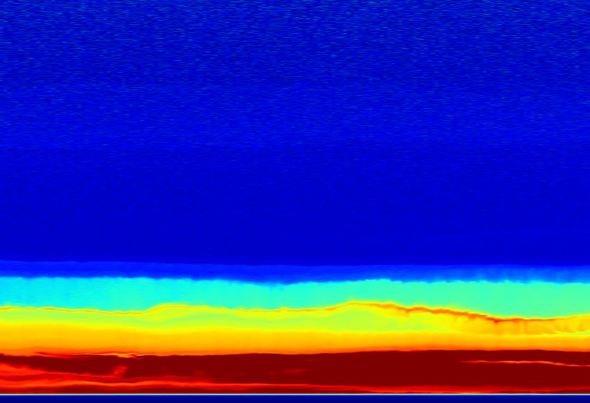
extremely suitable for the implementation within the single MUSA (40.60° N, 15.72° E, 760 m a.s.l.) 1e7
calculus chain (SCC), the EARLINET centralized processing 12 1.20
Range corrected signal at 1064 nm
suite. 1.05
10
0.90
Height a.s.l. [km]
8 0.75
[a.u.]
6 0.60
1 Introduction
0.45
4 0.30
The European Aerosol Research Lidar Network
(EARLINET; Pappalardo et al., 2014) operates Raman 2 0.15
lidars at a continental scale. Since the beginning, the net- 0.00
19:30 20:00 20:30 21:00 21:30 22:00
work aimed towards a sustainable observing system that has Time UTC
been achieved by developing a quality assurance strategy,
and optimizing instruments and data. To this direction and Figure 1. Temporal evolution of the 1064 nm range-corrected lidar
towards future advancement, the network plans continuous signal obtained with the MUSA system in Potenza on 14 July 2011,
measurements and near-real-time data delivery. With this in 19:20–22:10 UTC.
mind, the single calculus chain (SCC; D’Amico et al., 2015)
for automatic lidar analysis has been developed and cur-
rently delivers profiles of optical aerosol properties. The more accurate aerosol classification as well as insight into the
EARLINET SCC explores the implementation of new various aerosol types (Burton et al., 2013). Consequently, an
features like profiles of intensive optical properties and objective, multivariate analysis is needed to take advantage
determination of aerosol layer geometrical properties. The of this information. Automatic algorithms are, therefore, em-
intensive optical properties are type-dependent and can be ployed to classify aerosol into respective types. These proce-
used to classify the observed layers into aerosol types. The dures make use of various classifiers that are able to quantify
categorization into different types provides significant help the differences between the aerosol classes. In classification
to understand aerosol sources, their effects, and feedback analysis, the observations are allocated to a known number
mechanisms to improve the accuracy of satellite retrievals of groups, i.e. a supervised learning technique. Whereas in
and to quantify assessments of aerosol radiative impacts on cluster analysis, the groups are not known beforehand and
climate (Russell et al., 2014) by intercomparing numerical the classifier is tasked with it.
models such as NWP (Numerical Weather Prediction) and The measured values are evaluated by the classifica-
CTM (Chemical Transport Model) (Baklanov et al., 2014). tion function to find the group to which the individual
Thus, EARLINET, by providing multi-wavelength range- most likely belongs. Specifically, distance-based classifica-
resolved aerosol properties, has an added value for aerosol tion techniques (e.g., k nearest neighbor, support vector ma-
typing. In this study we present a flexible automatic method chine algorithms) are straightforward, i.e. the classification
to classify EARLINET data. depends on the distance from the target instance to the train-
Lidar systems are capable of identifying multiple lay- ing instance. The Mahalanobis distance classifier (Maha-
ers in the atmosphere owing to their high vertical resolu- lanobis, 1936) has a wide range of applications and can be
tion (on the order of tens of meters). Thus, lidar-based re- used to categorize data points, each representing an obser-
trievals can provide a separate classification for each layer vation, into classes that have predefined characteristics. The
and are not confined to columnar classifications as in the distances between the observation and the different classes
case of sun photometers. The lidar technique has proven are calculated, and then the observation is attributed to the
to be a robust tool to classify aerosols with its capabil- class for which the distance is the minimum.
ity of polarization-sensitive and multi-wavelength measure- The Mahalanobis-distance-based classification found
ments (Liu et al., 2008). Sophisticated lidars, such as the great applicability in aerosol studies. For instance, the algo-
High Spectral Resolution Lidar (HSRL) and the multi- rithm developed by Burton et al. (2012) makes use of four
wavelength Raman lidars, offer a multitude of intensive lidar intensive properties, namely the particle linear depolar-
parameters that characterize different aerosol types (e.g., ization ratio at 532 nm, the particle lidar ratio at 532 nm, the
Müller et al., 2007a; Burton et al., 2012; Groß et al., 2013). backscatter-related 532-to-1064 nm color ratio, and the ratio
Typically, the particle extinction-to-backscatter ratio (i.e., of particle linear depolarization ratios at 1064 and 532 nm
particle lidar ratio), the particle linear depolarization ratio at in order to classify aerosols into 8 types. A slightly differ-
one or more wavelengths, and the wavelength dependence of ent algorithm also including the uncertainties in the input
extinction and/or backscatter coefficients (i.e., extinction- or properties was introduced by Russell et al. (2014). Their al-
backscatter-related Ångström exponents) are considered. gorithm was applied to satellite-derived optical and physical
The increasing amount of available information and partic- data. The reference dataset was obtained from AERONET
ularly the plethora of lidar intensive parameters, can offer a (Aerosol Robotic Network; Holben et al., 1998) stations,
Atmos. Chem. Phys., 18, 15879–15901, 2018 www.atmos-chem-phys.net/18/15879/2018/N. Papagiannopoulos et al.: Automatic aerosol classification 15881
7
355 nm (532,1064)
532 nm (355, 532)
6 1064 nm
(355, 1064)
(355, 532)
Height a.s.l. [km] 5
4
3
2
1
0
0 0.0015 0.003 0 0.06 0.12 20 55 90 -1 0 1 2
Backscatter [km-1 sr -1 ] Extinction [km-1] Lidar ratio [sr]
Figure 2. Optical profiles measured in Potenza on 14 July 2011, 19:20–22:10 UTC, with a multi-wavelength Raman lidar. The error bars
correspond to the standard deviation.
where a single aerosol type tends to dominate (e.g., Cat- fication as well. Section 4 describes the testing phase and
trall et al., 2005). The pre-specified classes were then ap- provides a discussion of the results of the classification. The
plied to a 5-year record of retrievals from the spaceborne paper closes with conclusions of our study and suggestions
POLDER 3 (Polarization and Directionality of the Earth’s for further applications and improvements.
Reflectances 3; Tanré et al., 2011) polarimeter on PARA-
SOL (Polarization and Anisotropy of Reflectances for At-
mospheric Sciences coupled with Observations from a Lidar; 2 Operational network – EARLINET
Tanré et al., 2011) spacecraft. Recently, Hamill et al. (2016)
used the same classifier to produce an aerosol classification EARLINET (https://www.earlinet.org, last access: 10 Octo-
scheme based on long-term AERONET data. ber 2018) was established in 2000, providing aerosol pro-
In this work, we present a method analogous to the filing data on a continental scale, and is now part of the
one proposed by Burton et al. (2012), modified to fit EAR- Aerosols, Clouds, and Trace gases Research InfraStruc-
LINET’s needs and capabilities. The aerosol typing exclu- ture (ACTRIS; https://www.actris.eu/, last access: 3 October
sively makes use of EARLINET lidar-derived intensive prop- 2018). In these 18 years of continuous existence, EARLINET
erty data. We use the Mahalanobis distance as a classifier to has evolved both in the number of contributing stations and in
assign any given multi-dimensional observation to the pre- its observing capacity (Pappalardo et al., 2014). Currently, 30
specified aerosol class to which it is most similar. These stations are submitting aerosol extinction and/or backscatter
classes are defined using an EARLINET-based classifica- coefficient profiles to the EARLINET database, according to
tion scheme. The EARLINET classification scheme is pre- EARLINET’s measurement schedule (one daytime and two
sented in Sect. 2 where we also describe the parameters read- nighttime measurements per week). Therefore, these system-
ily delivered by the network that can be used to classify atic observations consolidate a 4-D European quantitative
aerosols. Furthermore, the major aerosol types that comprise and statistically significant aerosol survey. Further measure-
the aerosol classes onto which the aerosol classification is ments are devoted to special events, such as volcanic erup-
based are presented. In Sect. 3 the method that we apply to tions, forest fires, and desert dust outbreaks. Moreover, EAR-
EARLINET data is explained, and we present the training LINET provides correlative measurements during CALIPSO
phase. We set up a scheme for investigating the number of (Cloud-Aerosol Lidar and Infrared Pathfinder Satellite Ob-
aerosol classes and we perform an analysis to identify the servations) overpasses on each EARLINET station in or-
intensive parameters that contribute the most to the classi- der to validate satellite products (e.g., Mamouri et al., 2009;
Mona et al., 2009). Throughout the paper, we refer to mea-
www.atmos-chem-phys.net/18/15879/2018/ Atmos. Chem. Phys., 18, 15879–15901, 201815882 N. Papagiannopoulos et al.: Automatic aerosol classification
surements as a set of aerosol optical profiles reported in datasets can be found in, e.g., Müller et al. (2007a, b);
the EARLINET database that correspond to the same tem- Groß et al. (2011); Mona et al. (2012a); Navas-Guzmán
poral window, which typically extends for about 1 h. EAR- et al. (2013b), and Baars et al. (2016). For the time be-
LINET data are freely available through the ACTRIS web ing, there are different algorithms under development which
site (https://www.actris.eu/default.aspx, last access: 15 Oc- combine measurements and aerosol models (Nicolae et al.,
tober 2018) and are published to the CERA database (EAR- 2016; Wandinger et al., 2016). Nevertheless, automated
LINET publishing group 2000–2010, 2014a, b, c, d, e; EAR- observation-based algorithms working at the network level
LINET publishing group 2000–2015, 2018a, b, c, d, e). for the identification of layers, their boundaries, and the cor-
The majority of the EARLINET stations (67 % of the sta- responding aerosol typing are not yet available. The SCC tool
tions; Pappalardo et al., 2014) operate multi-wavelength Ra- for automatic processing of EARLINET lidar signals is, cur-
man lidars that combine a set of elastic and nitrogen in- rently, providing primarily profiles of particle extinction and
elastic channels, typically consisting of three elastic and backscatter coefficients, and volume and particle depolariza-
two inelastic Raman channels (the so-called 3β + 2α con- tion ratios. The SCC aims at incorporating modules for layer
figuration). In particular, they provide the aerosol extinc- identification, intensive properties retrieval, and aerosol typ-
tion (at 355 and 532 nm) and backscatter coefficients (at ing. Therefore, this paper could provide a starting point for
355, 532, and 1064 nm). This configuration allows for the a harmonized EARLINET classification tool that could also
retrieval of the range-resolved particle lidar ratio at 355 be used by other lidar networks, like the ones involved in
and 532 nm (Saer λ ). This intensive parameter depends on the GALION (GAW Aerosol Lidar Observation Network), the
shape, size, and chemical composition of the aerosol (Müller GAW (Global Aerosol Watch) initiative for the aerosol lidar
et al., 2007a). When lidar ratio is available for more than observation on a global scale, and within aerosol lidar studies
one wavelength, the corresponding color ratio can also be in general.
λ1 λ2
retrieved (Saer /Saer ). This quantity has shown the ability to
characterize the ageing status of smoke particles as well as 2.1 EARLINET manual aerosol classification
the spectral dependence of aerosol (Müller et al., 2007a;
Alados-Arboledas et al., 2011; Nicolae et al., 2013; Nepo- The typical procedure for aerosol categorization adopted
muceno Pereira et al., 2014). The combination of the optical within the EARLINET community consists of three main
data allows for the retrieval of the size-sensitive backscatter steps:
and/or extinction-related Ångström exponent and can be cal-
culated as 1. layer identification and cloud screening,
2. identification of the geometrical properties (boundaries,
ln[X(λ1 )/X(λ2 )] center of mass) of the aerosol layer, and
κX (λ1 , λ2 ) = (1)
ln(λ2 /λ1 )
3. the aerosol layer typing by means of investigation of
with X denoting the backscatter (β) or extinction coefficient intensive optical properties (Ångström exponents, lidar
(α) for a set of wavelengths, λ1 and λ2 . Moreover, 52 % of ratios, and particle linear depolarization ratios), model
EARLINET stations (Pappalardo et al., 2014) are equipped outputs (backward trajectory analyses), and ancillary in-
with depolarization channels, thus providing profiles of the strument data if available (e.g., satellite or sun photome-
particle linear depolarization ratio. It can be calculated ac- ter data).
cording to Biele et al. (2000) and Freudenthaler et al. (2009):
In what follows, an example of an aerosol type assign-
(1 + δm )δv R − (1 + δv )δm ment using EARLINET data is presented. Figure 1 shows the
λ
δaer = (2) temporal evolution of the range-corrected signal at 1064 nm
(1 + δm )R − (1 + δv )
from a measurement made in Potenza, Italy, on 14 July 2011,
with R being the backscatter ratio, δm the molecular depolar- 19:20–22:10 UTC with the reference lidar system MUSA
ization, and δv the volume depolarization ratio. This param- (Multiwavelength System for aerosol) of CNR-IMAA (Con-
eter provides information on the particle shape, thus enhanc- siglio Nazionale delle Ricerche – Istituto di Metodologie per
ing the aerosol typing strength of the network. Under favor- l’Analisi Ambientale). High values show a stratified aerosol
able conditions, the aerosol microphysical properties (such layer from the ground up to 5 km, whereas low values indi-
as the effective radius), the volume concentration, and the re- cate aerosol-free regions. The lowest altitude range presents
fractive index can also be retrieved through complex numer- the overlap between the laser beam and the receiver field
ical algorithms (e.g., Müller et al., 2004; Veselovskii et al., of view and, therefore, it is the blind range of the lidar.
2010; Bovchaliuk et al., 2016; Chaikovsky et al., 2016). MUSA has a full overlap at around 1.15 km a.s.l. for 1064 nm
The data products described above make the EARLINET (Madonna et al., 2015). The optically thicker layer lies be-
data an excellent basis to perform aerosol typing at the conti- low 2 km, with a distinct layer atop extending up to 3.5 km,
nental scale. Examples of methodologies to classify aerosol and, finally, an optically thinner region from 3.5 to 5 km.
Atmos. Chem. Phys., 18, 15879–15901, 2018 www.atmos-chem-phys.net/18/15879/2018/N. Papagiannopoulos et al.: Automatic aerosol classification 15883
The retrieved profiles for the same temporal window of par- Start date: 14/07/2011 – end date: 09/07/2011
ticle backscatter and extinction coefficient, lidar ratios, and Release height 2.0–3.5 km a.s.l.
Ångström exponents are shown in Fig. 2. The particle ex-
tinction and backscatter coefficient are given with their full 103
4 5° N
resolution. To calculate the lidar ratio, the backscatter coef-
ficient was smoothed in the same effective vertical resolu-
4 0° N
Sensitivity [s]
tion using a Savitzky–Golay second-order filter (Iarlori et al.,
2015) and only the useful range of signals was kept; the ef-
fective resolution of the resulting profiles varied from 120
3 5° N 102
to 480 m using the method described in Pappalardo et al. 3 0° N
(2004b). The layer 2.0–3.5 km has a constant behavior with
the range for the intensive optical profiles indicating the pres- 2 5° N 101
ence of the same type of particles. The mean values of all 0
3 0 ° E1 0
20° N
optical parameters in the range are calculated: lidar ratios of 20° W 10° W 0° 10° E 20° E
48 ± 4 sr at 355 nm and 53 ± 4 sr at 532 nm and Ångström
Figure 3. FLEXPART footprint for the air mass traveling below
exponents (i.e., κβ (355, 1064), κβ (532, 1064), κβ (355, 532), 2 km height and arriving at Potenza between 2.0 and 3.5 km at
and κα (355, 532)) of −0.3 to 0.4 were found. 22:00 UTC on 14 July 2011. The colors are coded with respect to
For the classification of aerosols with respect to their the logarithm of the integrated residence time in a grid box in sec-
source regions and age, auxiliary information like results of onds for a 5-day integration time.
transport and dispersion models or satellite data are used. For
the observed aerosol layer, the Lagrangian dispersion model
FLEXPART (FLEXible PARTicle dispersion model; Stohl The considered aerosol types almost coincide with the ones
et al., 2005) was used for a 5-day backward simulation. Fig- used in the CALIPSO classification scheme (Omar et al.,
ure 3 shows the so-called footprint that indicates the areas 2009), which already provides a satisfactory description of
of the air parcels traveling below 2 km before reaching the the atmospheric aerosol content. Moreover, adopting similar
study area. The model output is given in terms of the deci- classification schemes, the direct comparison of the proposed
mal logarithm of the integrated residence time in seconds in typing against the CALIPSO product is possible.
a grid box. The most probable aerosol source region and the
aerosol type were assigned accordingly. The dust-prone area 2.2.1 Continental
of northern Africa (Morocco and northern Algeria) along
with the Mediterranean Sea are most likely the sources of Man-made activities dictate the aerosol pattern within the at-
the observed layer and suggest a mixture of dust and marine mospheric boundary layer, and affect the observations in the
particles. The combined information of the backward trajec- lower troposphere in Europe. Anthropogenic particles show
tory analysis and the intensive property values indicate the a strong wavelength dependence of their optical properties,
presence of dust particles and they are in accordance with i.e., high Ångström exponent values. Moreover, they are typ-
the typical dust values observed over Potenza (Mona et al., ically small and do not significantly depolarize the backscat-
2014). 532 = 0.04 ± 0.04; Heese et al., 2016), and due
tered light (δaer
In the following, the characteristics of the major aerosol to the high carbon content, these particles reveal high lidar
types are presented. These aerosol types are used for the au- ratios (Giannakaki et al., 2010). Herein, we refer to this par-
tomatic classification and correspond to aerosol layers typi- ticle type as polluted continental.
cally encountered over Europe. Typically, the clean continental aerosol over Europe is a
mixture of anthropogenic pollution with particles from nat-
2.2 Aerosol types ural sources. The clean continental type shows a low de-
polarizing ability with values lower than 0.07 (Omar et al.,
One of the defining characteristics of the aerosol properties 2009); low lidar ratio values, i.e., 20–40 sr; and relatively
is the source; aerosols found in the atmosphere can be, for high Ångström exponents, i.e., 1.0–2.5 (Ansmann et al.,
example, mineral particles from arid areas of the Earth or 2001; Giannakaki et al., 2010). The clean continental, there-
organic carbon emitted during biomass burning events. Due fore, differentiates from the polluted continental type due to
to the multiple influence of the aerosol origin on the prop- lower lidar ratio values.
erties, aerosol sources can be used to classify them into dif-
ferent categories. In this section, we provide an overview of 2.2.2 Marine
the main aerosol types observed over the EARLINET sta-
tions followed by the corresponding optical properties. This Marine particles are produced at the sea surface and dom-
section also aims to provide important information on the inate the shallow boundary layer over the oceans (e.g.,
aerosol types that the automatic classification is based upon. O’Dowd and de Leeuw, 2007). Specifically, the sea-salt par-
www.atmos-chem-phys.net/18/15879/2018/ Atmos. Chem. Phys., 18, 15879–15901, 201815884 N. Papagiannopoulos et al.: Automatic aerosol classification
ticles feature a predominant coarse mode; however, they are et al. (2009); Córdoba-Jabonero et al. (2011); Preißler et al.
spherical in humid conditions and weakly absorbing in con- (2011); Valenzuela et al. (2012); Papayannis et al. (2014);
trast to the dust particles. Therefore, they yield low particle Binietoglou et al. (2015); Bravo-Aranda et al. (2015), and
lidar ratio values, are almost non depolarizing, and exhibit Granados-Muñoz et al. (2016a). The study of Papayannis
low Ångström exponent values (e.g., Burton et al., 2014; et al. (2008) indicated a large variability in the measured li-
Dawson et al., 2015). This aerosol type is mainly identifiable dar ratio and Ångström exponent values among the differ-
by the low particle lidar ratio, i.e., 15–25 sr at 532 nm (Bur- ent sites, suggesting mixing at different levels. Additionally,
ton et al., 2012). As marine aerosol layers manifest them- the mixture processes also produce large variability in in-
selves over water bodies, either stations only located at the tensive properties as measured at the same site (e.g., Mona
shorelines and under specific meteorological conditions or et al., 2006, 2014). As a consequence of the complex struc-
shipborne measurements can observe pure maritime parti- ture of the observed aerosols over Europe and the effects
cles. Consequently, the observations of pure maritime par- of transport and mixing on the properties of these particles,
ticles is rare within EARLINET and, generally, when these we consider the use of three dust groups: pure dust, mixed
particles are observed their characteristics are far from pris- dust, and polluted dust. The pure dust group refers to parti-
tine (Preißler et al., 2013; Papagiannopoulos et al., 2016a). cles for which the mixing with other aerosol types is neg-
However, mixtures with important contribution of marine ligible. Mixed dust refers to dust-dominated layers mixed
particles can be observed in the Mediterranean basin (Papa- with marine particles. This leads to less depolarizing, and
giannopoulos et al., 2016a). Thus, we consider pure marine less absorbing particles with respect to pure dust particles.
and marine-dominated layers as one single category denoted Several studies (Burton et al., 2012; Kim et al., 2013; Rogers
as mixed marine. et al., 2014; Papagiannopoulos et al., 2016a) have indicated
that this mixture is important and suggested its inclusion in
2.2.3 Mineral dust and dust mixtures the CALIPSO retrieval scheme for improving the accuracy
of aerosol backscatter and extinction coefficient profiles. Fi-
Mineral dust is produced in arid and semi arid regions of nally, the polluted dust category consists of dust-dominated
the world, and has a profound contribution to the total natu- mixtures with smoke and/or continental pollution, which pro-
ral aerosol loading (Ginoux et al., 2001). The optical prop- duce lower depolarization, higher lidar ratios, and enhanced
erties are considerably different from the other types, thus Ångström exponent values owing to the presence of small,
making them easy to identify. The irregular shape and the spherical particles (Groß et al., 2011; Burton et al., 2012;
large size (< 50 µm; Mahowald et al., 2014) lead to a signif- Tesche et al., 2013; Bravo-Aranda et al., 2015).
icant high depolarization of the backscattered radiation (e.g.,
532 = 0.34 ± 0.02 for Saharan dust over Germany; Wieg-
δaer 2.2.4 Smoke
ner et al., 2011), and to medium lidar ratio values (e.g.,
532 = 55 ± 10 sr; Tesche et al., 2013; Mona et al., 2014).
Saer Biomass burning is a major global source of atmospheric
They are spectrally neutral to backscatter and extinction, and aerosols. Generally, smoke particles are relatively small and
thus produce low Ångström exponent values (Wiegner et al., spherical that produce low depolarization, high Ångström ex-
2011). Therefore, the particle lidar ratio, particle linear de- ponents, and large lidar ratios (Amiridis et al., 2009; Baars
polarization ratio, and the Ångström exponent are excellent et al., 2012; Giannakaki et al., 2016). The optical prop-
physical parameters to characterize mineral dust and to dis- erties of smoke particles may vary due to the vegetation
tinguish it from other aerosol types. However, it needs to be type of the emitting source, the combustion type (smoul-
taken into account that the dust optical properties depend on dering or flaming fires), and atmospheric conditions (e.g.,
the source region and the transport pattern (Valenzuela et al., Balis et al., 2003). Furthermore, the particles are suscepti-
2014), which is a source of variability detected in the lidar ble to changes during their lifetime in the atmosphere (Nico-
ratio (e.g., Schuster et al., 2012; Nisantzi et al., 2015). Re- lae et al., 2013). Several EARLINET-based studies have fo-
cently, Mamouri et al. (2013) showed that dust originating cused on observations and characterization of smoke plumes
from the Arabian desert produced significantly lower lidar (e.g., Müller et al., 2005; Papayannis et al., 2008; Ansmann
ratio values (34–39 sr at 532 nm) than respective values (50– et al., 2009; Tesche et al., 2011; Alados-Arboledas et al.,
60 sr at 532 nm) from western Saharan dust particles. An 2011; Nepomuceno Pereira et al., 2014; Ancellet et al., 2016;
overview on the dust characterization using lidar measure- Ortiz-Amezcua et al., 2017), demonstrating that it is a fre-
ments can be found in Mona et al. (2012b). quently encountered aerosol type over Europe. In particu-
Dust can be transported over continental scales. In particu- lar, biomass burning aerosol originating from forest fires in
lar, Saharan dust outbreaks in Europe and across the Atlantic Canada and Siberia is regularly observed between May and
Ocean have been deeply investigated. The European conti- October (Amiridis et al., 2009; Sicard et al., 2012a; Ortiz-
nent is regularly influenced by advected Saharan particles as Amezcua et al., 2017). However, the similarities of the phys-
has been discussed by, e.g., Ansmann et al. (2003); Guerrero- ical characteristics of smoke particles and continental parti-
Rascado et al. (2008, 2009); Papayannis et al. (2008); Müller cles result in similar optical properties, making these types
Atmos. Chem. Phys., 18, 15879–15901, 2018 www.atmos-chem-phys.net/18/15879/2018/N. Papagiannopoulos et al.: Automatic aerosol classification 15885
difficult to distinguish. In this work, biomass burning parti- 3 Automatic aerosol type classification
cles are treated as a single category called smoke.
3.1 Methodology
2.2.5 Volcanic ash
We developed an automated typing method, based on the
Volcanoes are another important source of atmospheric work of Burton et al. (2012), but modified it in order to
aerosols. Volcanic eruptions eject great amounts of material be compatible with the database of EARLINET. Two ma-
in the atmosphere (tephra), while the fraction smaller than jor steps are identified in the proposed method: the train-
2 mm is labeled as volcanic ash. Most of these aerosols will ing (Sect. 3.2) and the testing (Sect. 4.1) phase. The first
settle only a few tens of kilometers away from the volcano step consists of the following procedures. As described in
but smaller particles can travel thousands of kilometers and Sect. 3.2.1, well characterized aerosol layers are manually
affect wider areas (Mattis et al., 2010; Sawamura et al., 2012; separated into classes based on their physical characteristics;
Sicard et al., 2012b; Navas-Guzmán et al., 2013a; Kokkalis the set of classes constitutes the reference dataset. This pro-
et al., 2013; Pappalardo et al., 2013). The optical proper- cedure involves the determination of each observed aerosol
ties of volcanic ash aerosols is generally similar to the one layer location and the estimation of mean layer intensive op-
of desert dust, as was shown by Ansmann et al. (2010) and tical properties. Based on this analysis, the classifying pa-
Wiegner et al. (2012) for fresh ash with particle linear de- rameters that provide the required information for a better
polarization ratios reaching 0.37 and lidar ratio at 532 sr of discrimination of the aerosol type are selected (Sect. 3.2.2).
50–65 sr. Aged volcanic particles as observed by Papayannis Next, in order to estimate how accurately a predictive model
et al. (2012) indicate less non-sphericity with depolarization will perform, the reference dataset is split into training and
ratio values of 0.1–0.25 and lidar ratios for 355 nm within validation datasets, and the application of the classifier is
the range 55–67 sr and for 532 nm 76–89 sr. More details can evaluated (Sect. 3.2.3). Section 3.2.4 describes the inference
be found in Mona and Marenco (2016) where the authors of characteristic depolarization values in the algorithm with
give a summary of how the intensive optical properties vary the intention to increase the prediction of the model. For the
as a function of time. Furthermore, volcanic eruptions inject second step, already pre-classified EARLINET data are used
sulfur dioxide into the atmosphere thus leading to sulfate to assess the performance of the automatic typing procedure.
particles. Pappalardo et al. (2004a) and Wang et al. (2008) Figure 4 illustrates the sequence of the proposed methodol-
reported lidar ratios of 50–60 sr at 355 sr and backscatter- ogy starting from the setting of the training dataset, up to the
related Ångström exponent of 2.7 (355 532), signature of assessment of the learning success during the testing phase.
sulfate particles originating from Mount Etna, Italy. More- Distance-based classification methods aim to assign an ob-
over, CALIPSO measurements indicated low particle depo- servation to a particular class based on the distance of the ob-
larization ratios for sulfate-rich volcanic clouds (Prata et al., servation from each class center. In general, the Mahalanobis
t
2017). Consequently, the difference in the optical properties distance between an observation x = x1 , . . ., xp and the
make lidar a powerful tool for volcano monitoring. However, t
mean class x = x 1 , . . ., x p in the p-dimensional space Rp
in this study sulfate particles and aged volcanic particles are is defined as
not considered. The aerosol type relevant to the airborne ash
refers to fresh ash and is denoted as volcanic ash. q
As an additional consideration, the defined aerosol types
DM (x, x) = (x − x)T S−1 (x − x), (3)
presented in Sect. 2.2 may not be representative of the en-
tire aerosol load and, apart from the dust mixtures, they do where S is the class covariance matrix. The surfaces identi-
not consider other aerosol mixtures. For example, this aspect fied by the equation DM = const. are ellipsoids that are cen-
can be observed in the definition of the volcanic category tered around the mean x. The main characteristic of the mul-
where the particles have different characteristics depending tivariate Mahalanobis distance is that it accounts for the vari-
on the transport pattern. The particles near the source have ance in each variable and the covariance between variables.
optical properties similar to desert dust whereas long-range- By contrast, the Euclidean distance treats all the variables in
transported volcanic plumes have altered properties due to the same way and the constant distance surfaces from a fixed
the sedimentation of the coarser particles. Therefore, it is point are represented by a sphere.
important to further include a more exhaustive aerosol class The Mahalanobis distance of an observation from an
analysis. aerosol class is estimated, and is assigned to the aerosol class
for which the distance is minimum. Two screening criteria
are applied to the minimum distance following the procedure
of Burton et al. (2012). The methodology uses 3 and 4 clas-
sifying parameters and the minimum accepted distance for a
measurement to be labeled is 4 and 4.3, respectively. More-
over, the normalized probability of the aerosol class needs
www.atmos-chem-phys.net/18/15879/2018/ Atmos. Chem. Phys., 18, 15879–15901, 201815886 N. Papagiannopoulos et al.: Automatic aerosol classification
Figure 4. Flowchart of the methodology. First, well characterized aerosol layers are grouped into meaningful classes that represent the
reference dataset: paper 1 (Papagiannopoulos et al., 2016a), paper 2 (Pappalardo et al., 2013), and paper 3 (Schwarz, 2016). Second, an
analysis is performed to determine the best performing classifying parameters among the available intensive parameters. Third, based on the
reference dataset the selected classifier is validated using the leave-one-out cross validation (LOOCV) procedure in order to ensure correct
aerosol type separation. Finally, the trained typing algorithm is applied to an independent and manually typed dataset (the testing dataset) for
the assessment of the algorithm performance. Note that both phases have been applied with and without the depolarization ratio.
to be higher than 50 %. Otherwise, the type assignment is Table 1. Number of classified aerosol layers adapted from Schwarz
difficult as the measurement can be equidistant from 2 or (2016). The mixtures category is comprised of two or more pure
more aerosol type classes, and possibly indicate the mixing aerosol types.
of these aerosol types.
Aerosol type All Only from
3.2 Training phase analyzed 3β + 2α
Clean continental (CC) 45 5
3.2.1 Dataset Polluted continental (PC) 95 19
Dust (D) 41 6
In supervised learning techniques, the reference dataset is Mixed dust (MD) 56 9
crucial to the overall predictive performance of the algo- Polluted dust (PD) 14 3
rithm. Therefore, it is fundamental to use well-characterized Smoke (S) 24 7
Volcanic (V) 21 4
EARLINET profiles. Namely, EARLINET aerosol classified
Mixtures 348 35
layers from Pappalardo et al. (2013); Papagiannopoulos et al.
Total 644 88
(2016a), and Schwarz (2016) were used and will be presented
below.
EARLINET observations from 2008 to 2010 were ana-
lyzed and the aerosol types were determined with respect to 3β + 2α”). The mixtures category includes all the mixtures
the source origin following a similar approach to Sect. 2.1 of two or more aerosol species without containing polluted
(Schwarz, 2016) and present the backbone of the refer- dust and mixed dust categories that are reported individually.
ence dataset. Table 1 lists the classified aerosol types of As discussed above, the requirement for 3β +2α lidar con-
the above study (644 individual aerosol layers) with respect figuration pinpoints the low occurrence (see Table 1) of some
to the aerosol types presented in Sect. 2.2; however, all aerosol types such as the clean continental, polluted dust,
these aerosol layers cannot be used given the need for the and dust. Furthermore, marine aerosol was not reported in
maximum optical properties available (column “only from the study and the volcanic layers do not reflect the volcanic
Atmos. Chem. Phys., 18, 15879–15901, 2018 www.atmos-chem-phys.net/18/15879/2018/N. Papagiannopoulos et al.: Automatic aerosol classification 15887
ash characteristics described in Sect. 2.2. Conversely, the lat- tal (CC), polluted continental (PC), pure dust (D), mixed dust
ter were volcanic layers found in the stratosphere and thus (MD = dust + marine), polluted dust (PD = dust + smoke
different from the fresh ash that we consider. In order that and/or dust + polluted continental), mixed marine (MM),
the aerosol classes include all the major aerosol components, smoke (S), and volcanic (V). However, some of these 8
the aforementioned aerosol types need to be enhanced with classes overlap consistently in the feature space. As a con-
other observations. Therefore, we implemented EARLINET sequence, we exploited the combined use of overlapping
network-wide typing results already published in the litera- aerosol types. Therefore, we merged the types that tend to re-
ture (Pappalardo et al., 2013; Papagiannopoulos et al., 2016a) flect the same aerosol characteristics, and hence we evaluate
for a total of 69 layers as the reference dataset. Note that the corresponding effects on the prediction rate of the algo-
calibrated particle linear depolarization ratio profiles are not rithm. Two pathways were followed. First, the smoke and the
available in the selected dataset. polluted continental categories were grouped into the more
The type-dependent mean properties are reported in Ta- generic type of small with high lidar ratio values. Second, all
ble 2 and coincide with the typical values as of those in the dust-like aerosol types were merged. The different group-
Sect. 2.2. However, aerosol classification is based on an inter- ing categories are summarized in Table 3.
pretative analysis of the retrieved optical properties and the
model simulations, and it is a qualitative method of type as-
3.2.2 Classifying parameters selection
signment. Thus, there is an inherent possibility of error in the
determination of the true aerosol type. This error, if made,
propagates into the automatic algorithm and the predicted Next, we performed a sensitivity analysis to identify which
aerosol class might deviate from the “truth” aerosol class. classifying properties provide the adequate information to
Specifically, dust and volcanic types present the same char- better predict the correct aerosol class. We used three aerosol
acteristics with Ångström exponents as low as 0, although intensive properties due to the lack of particle linear depolar-
dust lidar ratios are 58 ± 12 and 55 ± 7 sr for 355 nm and ization ratio profiles to evaluate the strength of the selected
532 nm, respectively, and are higher than the volcanic lidar classifier to discriminate among the predefined classes. Two
355 = 50 ± 11 and S 532 = 48 ± 13 sr). The Ångström
ratios (Saer statistical parameters are used: the total and the partial Wilks’
aer
exponents (i.e., κβ (355, 1064), κβ (532, 1064), κβ (355, 532), lambda (3; Wilks, 1963) that are widely used, e.g., Burton
and κα (355, 532)) for mixed dust are between 0.4 and 0.7 et al. (2012) and Russell et al. (2014). The total 3 statistic
and lidar ratio values are below 50 sr, whereas for polluted shows the tendency of the above set of pre-specified classes
dust the Ångström exponents lie within 0.6–1.0 and lidar ra- (or any subset of it) to separate. The partial 3 is calculated
tio values for 355 and 532 nm are 54±8 and 64±9 sr, respec- for each of the intensive properties separately and indicates
tively. This behavior reflects the mixing of dust with pollu- the discriminatory power of the used intensive property. For
tion/smoke that tends to decrease the size of the aerosol mix- both parameters, values range from 0 to 1. Values near 0
ture and increase its absorbing capacity. Polluted continen- show high discriminatory power while values near 1 show
tal and smoke reveal the same size characteristics with mean low discriminatory power.
Ångström exponents from all the available variables around The lowest total 3 was found to be 0.033 for the set
∼ 1.4 and ∼ 1.3, respectively. The smoke mean lidar ratio κβ (355, 1064), Saer532 , and S 532 /S 355 ; whereas the partial 3
aer aer
values present the higher ones among the aerosol types – i.e., 532 355 , 0.17 for κ , and 0.30 for S 532 . For this
is 0.51 for Saer /Saer β aer
81±16 and 78±11 sr for 355 and 532 nm, respectively – and dataset, the low 3 value for κβ indicates that this variable
the polluted continental values succeed with 69±12 and 63± has the most weight in the classification. The decision for the
13 sr for 355 and 532 nm, respectively. For clean continental, selected parameters stems solely from the lowest arithmetic
the Ångström exponents (i.e., κβ (355, 1064), κβ (532, 1064), value of the total 3. Therefore, for the other groups of pa-
κβ (355, 532), and κα (355, 532)) are between 1.0 and 1.7 and rameters the total 3 is equally low, ∼0.05, which indicates
lidar ratios, for 355 and 532 nm, are 50 ± 8 and 41 ± 6 sr. that a 2β + 2α lidar setup could also be equally used when
This characteristic separates clean continental from polluted the algorithm is trained with κβ (355, 532). With reference to
continental as the particles yield lower lidar ratio values. 532 and S 355 can be used interchangeably
the lidar ratio, the Saer aer
Finally, mixed marine particles are found to be relatively due to the almost equal total 3 (i.e., 0.034).
small in size with Ångström exponents (i.e., κβ (355, 1064), For the rest of the aerosol groups reported in Table 2, the
κβ (532, 1064), κβ (355, 532), and κα (355, 532)) in the range total and partial (for κβ ) 3 are, respectively, 0.036 and 0.18
0.8–1.0 and thus overlap with other aerosol types. The char- (7a classes), 0.041 and 0.18 (7b classes), 0.044 and 0.18 (6
acteristic parameter that defines the mixed marine category classes), 0.057 and 0.20 (5 classes), and 0.070 and 0.21 (4
is the lidar ratio, the values are found to be the smallest classes). The 3 shows good discriminatory power for each
532 = 24 ± 8 sr) among the aerosol types.
(Saer of the grouping classes, although there is a slight increase in
In the proposed method, the aerosol layers are classified in the values as the number of classes is reduced. This behavior
terms of the aerosol types described in Sect. 2.2. As a starting can be ascribed to the high variance in the combined aerosol
point for this study, we use 8 aerosol classes: clean continen- types which makes the classification less selective.
www.atmos-chem-phys.net/18/15879/2018/ Atmos. Chem. Phys., 18, 15879–15901, 201815888 N. Papagiannopoulos et al.: Automatic aerosol classification
Table 2. Reference dataset: mean type-dependent intensive properties along with the standard deviation.
Type κβ (355, 1064) κβ (532, 1064) κβ (355, 532) κα (355, 532) 355 (sr)
Saer 532 (sr)
Saer No. of layers
CC 1.0 ± 0.2 1.0 ± 0.3 1.3 ± 0.3 1.7 ± 0.6 50 ± 8 41 ± 6 9
PC 1.3 ± 0.3 1.3 ± 0.2 1.4 ± 0.6 1.7 ± 0.5 69 ± 12 63 ± 13 16
D 0.4 ± 0.1 0.4 ± 0.1 0.3 ± 0.2 0.3 ± 0.4 58 ± 12 55 ± 7 9
MD 0.5 ± 0.2 0.4 ± 0.3 0.7 ± 0.3 0.5 ± 0.3 42 ± 4 47 ± 6 10
PD 0.9 ± 0.3 0.8 ± 0.1 1.0 ± 0.5 0.6 ± 0.2 54 ± 8 64 ± 9 5
MM 0.8 ± 0.1 0.8 ± 0.2 1.0 ± 0.3 0.9 ± 0.3 25 ± 7 24 ± 8 8
S 1.3 ± 0.1 1.3 ± 0.1 1.2 ± 0.3 1.3 ± 0.3 81 ± 16 78 ± 11 7
V 0.1 ± 0.1 0.4 ± 0.3 0.2 ± 0.3 0.2 ± 0.3 50 ± 11 48 ± 13 5
Table 3. Aerosol types that constitute the classes investigated. CC stands for clean continental, PC stands for polluted continental, D stands
for dust, MD stands for mixed dust, PD stands for polluted dust, MM stands for mixed marine, S stands for smoke, and V stands for volcanic
particles.
No. types Groups of aerosol types
8 D V MD PD CC MM PC S
7a D+V MD PD CC MM PC S
7b D V MD PD CC MM PC+S
6 D+V MD PD CC MM PC+S
5 D+V+MD+PD CC MM PC S
4 D+V+MD+PD CC MM PC+S
Figure 5 shows the characteristics of the reference dataset tion (LOOCV) procedure, also referred to as holdout proce-
in terms of the Saer 532 and κ (355, 1064) for the 8 and 4 dure or simply cross validation, which is a degenerate case
β
aerosol classes that represent the maximum and minimum of the k fold cross validation, where k is chosen as the to-
aerosol groupings used. The coloring corresponds to the vari- tal number of samples (Rencher, 2002). The choice of the
ous classes and the crosshairs indicate the standard deviation procedure, even though computationally expensive, is used
of each of the aerosol layers. The 90 % confidence ellipses when datasets are sparse and trains the algorithm with as
are calculated using the eigenvalues and eigenvectors of the many observations as possible. Each measurement is sepa-
covariance matrix and define the region that contains 90 % of rately removed from the training dataset in order to compute
all the points that can be drawn from the underlying normal the classification rule, and this rule is used to classify the re-
class distribution. The various aerosol classes tend to popu- moved observation. The error rate is estimated as a percent-
late specific areas of the graph, whereas the overlap of the age of all incorrect predictions divided by the total number
neighboring classes is significant, although the classes are of the reference dataset, and is equivalent to 1 minus accu-
better pinpointed as long as we merge classes with similar racy. Values near 0 show high predictive performance while
characteristics. However, the latter does not reflect the ob- values near 1 show low predictive performance. For the clas-
tained values of the statistical parameters (total 3 increased sification options of the Table 3, the error rate, expectedly,
from 0.033 for 8 classes to 0.070 for 4 classes), and, as ex- decreases with decreasing number of aerosol classes (39 %
plained above, the reference dataset very well delineates the for 8 classes, 36 % for 7a classes, 30 % for 7b classes, 28 %
aerosol types and by combining the neighboring types the for 6 classes, 19 % for 5 classes, and 10 % for 4 classes). It
variance increases. should be mentioned that the typing in multiple classes and
typing accuracy are two conflicting aspects. The choice of 8
3.2.3 Validation of the classifier aerosol classes appears to be sufficient to describe the major
aerosol components, but ostentatious for a 3β +2α lidar con-
figuration. Four classes, on the other hand, provide a coarse
In order to evaluate the predictive accuracy of the automatic
aerosol characterization and the prediction accuracy of the
method, it is needed to split the initial reference dataset into
algorithm is expected to increase.
a training and a validation dataset. Like this, we use the train-
ing dataset to calculate the classification functions and then
submit each observation in the validation dataset to the clas-
sification function obtained from the training dataset. For
this study, we make use of the leave-one-out cross valida-
Atmos. Chem. Phys., 18, 15879–15901, 2018 www.atmos-chem-phys.net/18/15879/2018/N. Papagiannopoulos et al.: Automatic aerosol classification 15889
8 aerosol classes 4 aerosol classes
120 120
S S+PC
100 100
PD D+PD+MD+V
80 D 80
S 532
aer
[sr] 60 PC 60
40 40
CC CC
V
20 20
MD MM MM
0 0
0 0.5 1 1.5 2 0 0.5 1 1.5 2
κ β (355,1064) κ β (355,1064)
Figure 5. Colored pre-specified classes and 90 % confidence ellipses for 8 and 4 aerosol classes. The error bars correspond to the standard
deviation of the selected mean intensive properties. CC stands for clean continental, D stands for dust, MD stands for mixed dust, MM stands
for mixed marine, PD stands for polluted dust, PC stands for polluted continental, S stands for smoke, and V stands for volcanic particles.
3.2.4 Algorithm training including particle Table 4. The mean and standard deviation of the particle depolar-
depolarization ratio ization ratio used for the pre-specified classes and the corresponding
bibliographic references.
Several studies have shown the unique information pro- Type 532
δaer References
vided by depolarization measurements (e.g., Liu et al., 2008;
Clean continental 0.04 ± 0.02 Burton et al. (2013)
Tesche et al., 2013; Burton et al., 2014), thus making this Polluted continental 0.05 ± 0.03 Burton et al. (2013)
intensive property a robust means to discriminate the vari- Dust 0.30 ± 0.01 Groß et al. (2011)
ous aerosol types. Valuable typing information can also be Mixed dust 0.15 ± 0.02 Groß et al. (2016)
obtained by the color ratio of the particle depolarization ra- Polluted dust 0.20 ± 0.05 Burton et al. (2013)
tios when more depolarization channels exist (Burton et al., Marine 0.03 ± 0.01 Groß et al. (2013)
2015). As already stated in Sect. 2, the majority of the sta- Smoke 0.10 ± 0.04 Burton et al. (2013)
tions perform depolarization measurements, and profiles are Volcanic 0.33 ± 0.03 Pappalardo et al. (2013)
routinely delivered by SCC. However, the reference dataset
does not contain depolarization information because it has
been released before the assessment of the quality assurance 532 are 0.55, 0.34, 0.52, and 0.12, respectively. The values
δaer
procedures within EARLINET. Therefore, a method appli- 532 as the most important
found for the partial 3 confirm the δaer
cable to EARLINET data collected since 2000 is proposed classifying parameter for the considered dataset. For the rest
in this work. We investigate the effect of adding depolariza- of the aerosol groups, the total and partial (for depolarization
tion information to the described method as the next releases ratio) 3 are, respectively, 0.005 and 0.14 (7a classes), 0.005
of EARLINET dataset will contain quality assured particle and 0.12 (7b classes), 0.006 and 0.14 (6 classes), 0.040 and
depolarization profiles and can be used for more accurate 0.68 (5 classes), and 0.050 and 0.69 (4 classes).
aerosol typing. To complement the reference dataset in this For the sake of completeness, the LOOCV method was
context, we used general literature values for particle linear also performed and the error rate was calculated. Figure 6
depolarization ratio at 532 nm (Table 4) in order to train the comparatively presents the training of the algorithm when
algorithm. For the clean continental type, the values ingested depolarization information is available and when not in terms
in the algorithm are retrieved from Burton et al. (2013) and of the total, partial 3, and the error rate of the LOOCV
refer to the polluted marine category. The decision for this method. The figure highlights the strength of polarization-
inconsistency stems from the shortage of clean continen- sensitive observations, while for the 5 and 4 classes (Fig. 6b)
tal particle depolarization values in the literature; however, the particle linear depolarization ratio becomes less impor-
the reported values coincide with the type characteristics de- tant (in this case the highest weight in the classification cor-
scribed in Sect. 2.2 and the values used in the CALIPSO typ- responds to the lidar ratio at 532 nm) due to the fact that
ing scheme (Omar et al., 2009). only one dust type represents volcanic and other dust mix-
In this case, the particle linear depolarization ratio was tures. Figure 7 presents cumulative bar plots with the median
added to the classifying parameters. Values within the (black dots), the 25–75 percentile (box), the 5–95 percentile
aerosol type range were randomly assigned to each sample (whiskers) for all four classifying parameters. The figure
and the 3 distribution was calculated. Total 3 is 0.004. The highlights the discriminatory power of δaer 532 , κ (355, 1064),
β
value of partial 3 for κβ (355, 1064), Saer532 , S 532 /S 355 , and 532 532 355
and Saer , whereas the Saer /Saer performs the worst. Further-
aer aer
www.atmos-chem-phys.net/18/15879/2018/ Atmos. Chem. Phys., 18, 15879–15901, 201815890 N. Papagiannopoulos et al.: Automatic aerosol classification
0.1
With depolarization
(a)
0.08
0.06 Without
Total
0.04
0.02
0
8 7a 7b 6 5 4
1
(b)
0.8
0.6
Partial
0.4
0.2
0
8 7a 7b 6 5 4
50
(c)
LOOCV [%]
40
Error rate of
30
20
10
0
8 7a 7b 6 5 4
No. of classes
Figure 6. Bar plots showing (a) the total 3, (b) the partial 3, and (c) error rate of LOOCV when comparing the training of the algorithm
532 /S 355 , S 532 , and κ (355, 1064)) and without (i.e., δ 532 , S 532 , and κ (355, 1064)) particle linear depolarization values. For
with (i.e., Saer aer aer β aer aer β
the partial 3, the brown bars correspond to the backscatter-related Ångström exponent and orange one to the particle linear depolarization
ratio because they represent the most significant classifying parameter of the classification.
more, the figure depicts the discriminatory power of the clas- tensive parameters for each available category in accordance
sifying parameter among the dust-like aerosol classes; how- with Table 2.
ever, the particle depolarization ratio seems to have no power
to separate the non-dust classes as discussed above. 4.2 Application of the methodology to EARLINET
data – case studies
4 Results To showcase the steps of the automatic classification, we
apply it to two selected cases for the 8 classes and for the
532 /S 355 , S 532 , and κ (355, 1064).
classifying parameters: Saer
4.1 Testing phase aer aer β
For the case in Sect. 2.1, the automatic algorithm labeled the
As a next step, an assessment of the predictive performance aerosol layer as dust, DM = 1.2 and the normalized proba-
of the pre-trained algorithm is made by using a testing bility 55 %. This coincides with our findings and highlights
dataset. For this, EARLINET data collected during the AC- the strength of the classification, albeit this example corre-
TRIS Summer 2012 intensive measurements (Sicard et al., sponds to a pure aerosol layer with no level of mixing with
2015; Granados-Muñoz et al., 2016b) were chosen to test the other aerosol types.
automatic typing algorithm. The measurements took place in The second case refers to a more complicated aerosol
the period of 8 June–17 July 2012 and were dedicated to Sa- scene. The Athens EARLINET station (Fig. 8) on
haran dust studies and also featured two field campaigns such 22 May 2014 observed an aerosol layer mostly in the height
as PEGASOS (Pan-European Gas-AeroSOl-climate inter- range between 1.5 and 3 km (Papayannis et al., 2016). Within
action Study) and CHArMEx (Chemistry-Aerosol Mediter- this layer the mean value of backscatter-related Ångström
ranean Experiment). During that period, 157 measurements exponent (355 1064) is 0.9 ± 0.1. The lidar ratio presents
were performed, out of which 42 measurements delivered mean values in the layer 40 ± 7 and 39 ± 6 sr at 355 and
3 backscatter and 2 extinction coefficient profiles. The de- 532 nm, respectively. The color ratio of the lidar ratios shows
scription of aerosol type distribution over Europe during a wavelength-independent layer with values of 1.1±0.2. The
the campaign was obtained following the procedure shown retrieved error corresponds to the standard deviation of the
in Sect. 2.1 (Papagiannopoulos et al., 2016b). The testing retrieved quantity calculated within the layer.
dataset comprises of 47 layers, 21 of which yield depolariza- In the following, a 6-day FLEXPART backward trajectory
tion ratio values. Table 5 provides the mean values of the in- indicates the pattern of the origin of air masses. Figure 9
Atmos. Chem. Phys., 18, 15879–15901, 2018 www.atmos-chem-phys.net/18/15879/2018/You can also read


