Topographic controls on divide migration, stream capture, and diversification in riverine life - ESurf
←
→
Page content transcription
If your browser does not render page correctly, please read the page content below
Earth Surf. Dynam., 8, 893–912, 2020
https://doi.org/10.5194/esurf-8-893-2020
© Author(s) 2020. This work is distributed under
the Creative Commons Attribution 4.0 License.

              Topographic controls on divide migration, stream
                 capture, and diversification in riverine life
          Nathan J. Lyons1 , Pedro Val2 , James S. Albert3 , Jane K. Willenbring4 , and Nicole M. Gasparini1
              1 Department   of Earth and Environmental Sciences, Tulane University, New Orleans, LA, USA
                       2 Department   of Geology, Federal University of Ouro Preto, Ouro Preto, Brazil
                     3 Department of Biology, University of Louisiana at Lafayette, Lafayette, CA, USA
               4 Scripps Institution of Oceanography, University of California San Diego, La Jolla, CA, USA

                                  Correspondence: Nathan J. Lyons (nlyons@tulane.edu)

                                Received: 16 October 2019 – Discussion started: 24 October 2019
                       Revised: 9 August 2020 – Accepted: 2 September 2020 – Published: 26 October 2020

      Abstract. Drainages reorganise in landscapes under diverse conditions and process dynamics that impact biotic
      distributions and evolution. We first investigated the relative control that Earth surface process parameters have
      on divide migration and stream capture in scenarios of base-level fall and heterogeneous uplift. A model built
      with the Landlab toolkit was run 51 200 times in sensitivity analyses that used globally observed values. Large-
      scale drainage reorganisation occurred only in the model runs within a limited combination of parameters and
      conditions. Uplift rate, rock erodibility, and the magnitude of perturbation (base-level fall or fault displacement)
      had the greatest influence on drainage reorganisation. The relative magnitudes of perturbation and topographic
      relief limited landscape susceptibility to reorganisation. Stream captures occurred more often when the channel
      head distance to divide was low. Stream topology set by initial conditions strongly affected capture occurrence
      when the imposed uplift was spatially heterogeneous.
         We also integrated simulations of geomorphic and biologic processes to investigate relationships among topo-
      graphic relief, drainage reorganisation, and riverine species diversification in the two scenarios described above.
      We used a new Landlab component called SpeciesEvolver that models species at landscape scale following
      macroevolutionary process rules. More frequent stream capture and less frequent stream network disappearance
      due to divide migration increased speciation and decreased extinction, respectively, especially in the heteroge-
      neous uplift scenario in which final species diversity was often greater than the base-level fall scenario. Under
      both scenarios, the landscape conditions that led to drainage reorganisation also controlled diversification. Across
      the model trials, the climatic or tectonic perturbation was more likely in low-relief landscapes to drive more ex-
      tensive drainage reorganisation that in turn increased the diversity of riverine species lineages, especially for the
      species that evolved more rapidly. This model result supports recent research on natural systems that implicates
      drainage reorganisation as a mechanism of riverine species diversification in lowland basins. Future research
      applications of SpeciesEvolver software can incorporate complex climatic and tectonic forcings as they relate to
      macroevolution and surface processes, as well as region- and taxon-specific organisms based in rivers and those
      on continents at large.

Published by Copernicus Publications on behalf of the European Geosciences Union.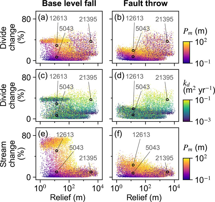
894          N. J. Lyons et al.: Topographic controls on divide migration, stream capture, and diversification in riverine life

1   Introduction

Topographic structure is primarily controlled by climate, tec-
tonics, and lithological erodibility (Whipple, 2004; Anders
et al., 2008; Han et al., 2015; Perron, 2017). Spatiotempo-
ral variability in these controls can induce spatially variable
erosion rates that can alter the planform topology of drainage
networks and the longitudinal profiles of channels in regions
with only metres to thousands of metres of relief (Gilbert,
1877; Giachetta et al., 2014; Forte et al., 2016; Willett et al.,
2014; Whipple et al., 2017). Drainages reorganise by divide
migration, which is the progressive movement of a drainage
divide, and stream capture that occurs when a portion of a
stream network loses connectivity to its former network as
it joins an adjacent network (Fig. 1; Bishop, 1995). Climat-
ically and tectonically induced changes to base level, wa-
ter flow direction, and erosional processes can alter topo-
graphic structure and reorganise drainages in settings such         Figure 1. Conceptual model of drainage reorganisation and river-
as internally draining fault-bounded basins (D’Agostino et          ine species macroevolution. Three stream networks exist in a hypo-
al., 2001), precipitation gradients (Bonnet, 2009), transient       thetical landscape at time T0 (a). Riverine species A.0 inhabits the
passive margins (Prince et al., 2011; Moodie et al., 2018), in-     lower-left stream network and B.0 inhabits the lower-right network.
tercontinental strike-slip faults (Guerit et al., 2016), and lat-   Drainages reorganised between T0 and a later time, T1 . Reorganisa-
eral variations in lithologic erodibility (Gallen, 2018; Harel      tion was carried out by a stream capture whereby a network segment
et al., 2019). Yet little attention has been paid to the impact     broke off the lower-left network and joined the upper network (b).
                                                                    Members of species A.0 that existed in the captured segment dis-
of drainage reorganisation on riverine biota despite the long-
                                                                    persed throughout the upper network, creating two populations of
standing recognition of their interactions (Bishop, 1995; Al-       this species in distinct stream networks that speciated child species
bert et al., 2018).                                                 A.1 and A.2. Drainage reorganisation also led to the stream network
    Topographic relief links climatic and tectonic forcings to      of B.0 disappearing, driving the extinction of this species. The lin-
biological evolution (Badgley et al., 2017). High rates of up-      eage history of the species before and after drainage reorganisation
lift and erosion are found in regions with great relief and high    is presented in a phylogenetic tree (c). After Albert et al. (2011).
diversity in many groups of terrestrial organisms, such as
birds and mammals (Simpson, 1964; Rahbek, 1997; Grenyer
et al., 2006). Relief enlarges environmental gradients and of-      richness in a geographically circumscribed region (e.g. is-
fers varied habitats, among other factors that form and main-       land, drainage basin) is a function of speciation, extinction,
tain diversity (Badgley et al., 2017). Conversely, riverine         dispersal (species geographic range expansion) (Hubbell,
groups, notably fish, are often most diverse in lowland basins      2001), and evolutionary time (Rabosky, 2009). Species dis-
where relief is low (Hoeinghaus et al., 2004; Muneepeer-            persal affects gene flow among populations and genetic di-
akul et al., 2008). The “river capture hypothesis” of Albert et     versity within populations, and the probability of species ex-
al. (2018) puts forth the idea that large and frequent drainage     tinction increases when dispersal ability is limited. Long-
captures in lowland basins contribute to high diversity of fish     term geographic separation of populations (i.e. allopatry) is a
in these regions. The challenges in testing this hypothesis in-     mechanism of speciation as populations genetically diverge
clude relating species-dense assemblages of riverine organ-         due to reproductive isolation (Coyne, 1992).
isms to limited records of drainage reorganisation. Mech-              Recent research implicates drainage reorganisation in the
anistic models of biologic and geomorphic processes can             evolutionary origin and ecological maintenance of high river-
provide information on complex process interactions, poten-         ine biological diversity in many regions (e.g. Waters and
tially guiding future empirical studies on the river capture        Wallis, 2000; Albert and Crampton, 2010; Bossu et al., 2013;
hypothesis and other lines of inquiry on the intersection of        Roxo et al., 2014; Craw et al., 2016; Albert et al., 2018;
landscapes and biodiversity.                                        Gallen, 2018). In the context of drainage reorganisation, the
    From a macroevolutionary perspective, regional biodiver-        organisms of a species can disperse across a greater area
sity is characterised by species richness (the number of            when a stream network expands by divide migration (Fig. 1;
species) in a clade (a group of organisms, e.g. a species,          Burridge et al., 2008). Divide migration can also cause net-
descending from a common ancestor) arising from the pro-            works to shrink, which increases the likelihood of species
cesses of speciation (species lineage splitting and forming         extinction (Grant et al., 2007). Stream capture increases spe-
new species) and extinction (species lineage termination)           ciation probability and lineage diversity in riverine taxa fol-
(Stanley, 1979). From a biogeographic perspective, species          lowing basin fragmentation (Burridge et al., 2006; Kozak et

Earth Surf. Dynam., 8, 893–912, 2020                                                    https://doi.org/10.5194/esurf-8-893-2020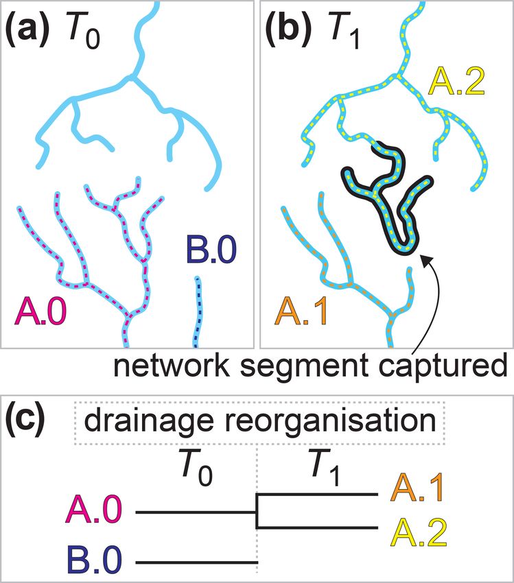
N. J. Lyons et al.: Topographic controls on divide migration, stream capture, and diversification in riverine life            895

al., 2006; Tagliacollo et al., 2015; Waters et al., 2015; Craw et   2   Description of modelling tools
al., 2016) and lowers extinction risk following basin integra-
tion by allowing the geographic range of species to expand          We built an LEM for this study using the Landlab mod-
(Grant et al., 2007, 2010).                                         elling toolkit (Hobley et al., 2017; Barnhart et al., 2020).
   Computational modelling is increasingly used to in-              This scientific computing software provides tools to build
vestigate landscape and biological evolution, although              two-dimensional numerical models of Earth surface dynam-
largely separately. Landscape evolution modelling has il-           ics. A landscape is represented by a model grid with config-
luminated drainage reorganisation in response to tectonic           urable spatial dimensions that Landlab users can easily set
strain (Castelltort et al., 2012), spatially variable bedrock       with built-in routines. Processes are implemented as model
erodibility (Giachetta et al., 2014), and autogenic pro-            components that control the values of fields, which are data
cesses (Pelletier, 2004), among other causative factors. Im-        associated with spatial elements of the grid, including a field
plementing captures in models has included probabilistic            of topographic elevation stored at grid nodes. Processes are
(Howard, 1971), numerical (Whipple et al., 2017), and cou-          effectively coupled when model components interact with
pled numerical–analytical (Goren et al., 2014) approaches.          the same fields. Landlab is open source, written in the Python
Models have also been used to demonstrate quantitative tech-        programming language, and available for download at https:
niques to identify regions undergoing drainage reorganisa-          //landlab.github.io (last access: 14 June 2020). Landlab ver-
tion (Willett et al., 2014; Forte and Whipple, 2018). Mean-         sion 2.0 was used in this study.
while, species richness has been simulated as an output of             We used a new Landlab component called SpeciesEvolver
spatially explicit ecological models that have static topog-        that enables researchers to model biological macroevolu-
raphy and that do not include tectonic or geomorphic pro-           tion in response to landscape change. This software evolves
cesses (Gotelli et al., 2009; Rangel et al., 2018). Salles et       taxonomic objects (e.g. populations, species) at geologic,
al. (2019) used landscape evolution models to quantify the          macroevolutionary, and landscape scales (Lyons et al., 2020).
connectivity of landscape portions, with implications for bio-      Each taxonomic object has at minimum a geographic range
diversity. However, computational models that integrate bio-        within the model grid, macroevolutionary rules, and a lin-
logical evolution with numerically implemented surface pro-         eage, all of which can be influenced by landscape properties
cesses have yet to be used in published research to our knowl-      and processes. For example, surface processes drive topo-
edge.                                                               graphic change, which may alter habitat connectivity that in
   In this paper we first investigate the conditions and pa-        turn influences the macroevolutionary processes of the simu-
rameter space in which drainages reorganise in response to a        lated taxon.
single perturbation in modelled landscapes. We address the             Taxa are implemented as object classes in the source code
following questions. Are landscapes with low or high topo-          of SpeciesEvolver. The base class provides behaviour and
graphic relief more susceptible to drainage reorganisation?         properties that can be expanded or overridden. Users can
What process parameters influence this susceptibility for           create classes of alternative and more complex taxa that in-
landscapes with a given relief? These questions are explored        herit from the base class, which saves users from recoding
with simulations of the surface processes most often used           behaviour already implemented in the software. Users may
in a landscape evolution model (LEM), namely stream inci-           make essentially limitless modifications – some more readily
sion and hillslope diffusion. Some processes potentially im-        implemented than others – including requiring a timeframe
portant to stream capture (e.g. inter-basin groundwater flow,       for an isolation period for a fragmented taxon to spawn new
mass wasting) are not included in this study. We also investi-      taxa and probabilistic-based rule adaptations for macroevo-
gate the conditions and parameter space in which the lineages       lution processes. In this study, we use the only taxon class
of species diversify in response to topographic changes. The        currently distributed with SpeciesEvolver called ZoneTaxon.
species represent those that live in or are closely associated      Instances of this class are associated with zone objects that
with drainage networks, e.g. the organisms that are adapted         manage the location of the taxa in the grid. The location of
to the channels, floodplains, or riparian forests of streams.       zones can be set using elevation ranges, landforms, or other
We integrate three macroevolutionary processes (dispersal,          attributes defined by the user. Our use of SpeciesEvolver for
speciation, and extinction) into an LEM to ask the following.       stream-based species in this study is described in Sect. 3.
Do the same parameters that lead to drainage reorganisation
also impact riverine species diversity within a landscape? In-      3   Experiment design
vestigating these three questions together allows us to asso-
ciate patterns of topographic change with diversification and       We investigated the questions posed in Sect. 1 using a model-
apply the new modelling tool, SpeciesEvolver. Through this          based experiment. Drainage reorganisation was triggered by
investigation we provide a framework for future model-based         perturbing the simulated topography in two model scenar-
research of the biological macroevolution that can follow the       ios: a base-level fall scenario with an instantaneous drop in
surface processes often included in LEMs.                           elevation along one model grid boundary and a fault throw
                                                                    scenario with an instantaneous block uplift of half of the

https://doi.org/10.5194/esurf-8-893-2020                                                 Earth Surf. Dynam., 8, 893–912, 2020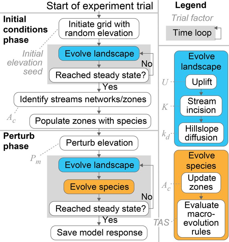
896              N. J. Lyons et al.: Topographic controls on divide migration, stream capture, and diversification in riverine life

Table 1. Parameters of model trials.                                     SALib (Herman and Usher, 2017). Variance-based meth-
                                                                         ods (1) analyse sensitivity globally throughout the parame-
      Constant                                                           ter space, rather than local methods that analyse sensitivity
      Time step                            1000 years                    around a point in the parameter space, and (2) decompose
      Drainage area exponent, m            0.5                           the variance of a response due to variation in the model fac-
      Channel slope exponent, n            1.0                           tors. The sensitivity of an output response to input factors
                                                                         is quantified using Sobol indices. The relative contribution
      Sensitivity analysis factor
                                                                         of Xi to the response variance is the Sobol first-order sensi-
      Initial topography seed              1–20 000                      tivity index,
      Uplift rate, U                       10−5 –10−3 m yr−1
      Erodibility coefficient, K           10−6 –10−4 yr−1                      Var (E [Y |Xi ])
                                                                         Si =                    ,                                   (2)
      Diffusion coefficient, kd            10−3 –10−1 m2 yr−1                       Var(Y )
      Critical drainage area, Ac           5 × 10⁵ –5 × 10⁶ m2
                                                                         where E[Y |Xi ] is the conditional expectation of Y given Xi .
      Perturbation magnitude, Pm           10−1 –102 m
                                                                         The first-order index does not include interaction among fac-
      Time to allopatric speciation, TAS   103 –105 years
                                                                         tors to influence the response. The second-order sensitivity
                                                                         index includes the interaction of Xi and Xj as
model grid. We predict that major perturbation-driven topo-

                                                                                Var E Y |X\i , X\J
graphic changes will lead to drainage reorganisation, which              Sij =                        ,                            (3)
                                                                                       Var(Y )
in turn will affect species diversification. We conducted sen-
sitivity analyses to identify the model input variables that             where X\i and X\j are all factors excluding Xi and Xj , re-
contributed most strongly to the variation of drainage reor-             spectively. The total effect of Xi including interactions is the
ganisation and species diversification as the inputs changed.            total-order sensitivity index as
The intent of these analyses is to describe key relationships
among model inputs and outputs given the modelled pro-                              Var E Y |X\i
                                                                         STi = 1 −                     .                              (4)
cesses and wide parameter space. Henceforth we use the term                              Var(Y )
“factor” to refer to a model input parameter that was varied in          In this study we use Sobol indices to rank the relative influ-
the sensitivity analyses and the term “response” to refer to a           ence that factors have on controlling model response vari-
model output variable investigated in the analyses. Each sce-            ables under the conditions of the two scenarios. The total-
nario was composed of 25 600 trials, which was the number                , first-, and second-order Sobol indices were calculated for
of trials necessary for the total-order Sobol index (described           each response in each scenario. For a given response (e.g.
in Sect. 3.1) to decrease below 1 % as more trials were run.             topographic relief described in Sect. 3.2.1), the ranking of
The scenarios only differed by the perturbation mechanism.               first-order indices indicates the relative influence that each
Each trial of a given scenario differed only by the values of            factor individually contributed to the response variance. The
the seven sensitivity analysis factors presented in Table 1 and          second-order index indicates the combined influence of two
described in Sect. 3.2.                                                  factors on the response. The total-order index encapsulates
                                                                         the total variance of the model response including first- and
3.1     Sensitivity analyses                                             higher-order interactions. For example, a factor with a large
We conducted a sensitivity analysis of each model response               total-order index and small first-order index indicates a re-
for both scenarios. A model response, Y can be represented               sponse is influenced through higher-order interaction of mul-
with the function f as                                                   tiple factors. A simple way to conceptualise these indices is
                                                                         that they act as the percent contribution of model factors to
Y = f (X1 , . . ., Xc ) ,                                         (1)    output variance. The sum of the contributions of the total-
                                                                         order indices can be greater than 100 % because the vari-
where {X1 , . . . , Xc } is the factor set, and c is the count of fac-   ances of interactions among the factors are included more
tors in this set. The factor sets for the experiment trials were         than once in the summation.
generated using a quasi-random Sobol sequence (Sobol,
1967). This sequence distributes factor values throughout the
                                                                         3.2    Model trial progression
parameter space more uniformly than a purely random se-
quence. The sensitivity analysis benefits from a uniformly               The base-level fall and fault throw scenarios proceeded in the
distributed parameter space because the response is better               same way. Only the mechanisms that perturbed the topogra-
characterised when the model is parameterised throughout                 phy differed between the two scenarios. A model grid with
the interval of all factors.                                             steady-state elevation and streams seeded with species was
   We used the variance-based Sobol (2001) sensitivity anal-             established during the initial conditions phase. The first ac-
ysis method implemented in the sensitivity analysis library,             tion in the perturb phase was either dropping the base level or

Earth Surf. Dynam., 8, 893–912, 2020                                                          https://doi.org/10.5194/esurf-8-893-2020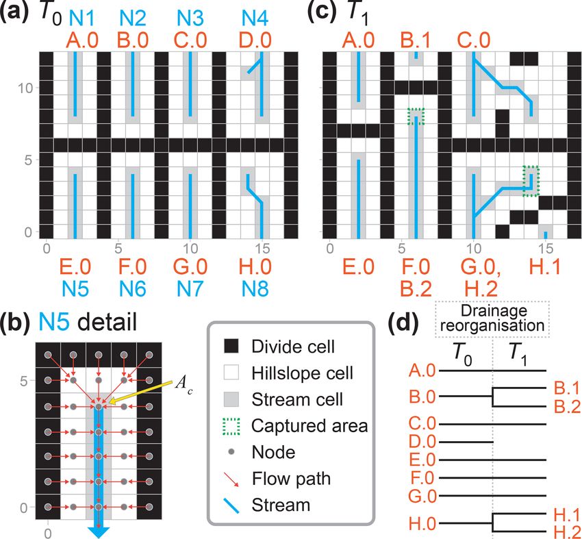
N. J. Lyons et al.: Topographic controls on divide migration, stream capture, and diversification in riverine life 897
developed from that noise. The initial noise is necessary for
streams to develop. The noise was generated using a pseu-
dorandom number generator that set the initial elevations of
grid nodes to values between 0 and 1 m. At each grid node the
generator selected a number randomly by performing opera-
tions on a previously generated value. The first number gen-
erated was computed using a seed value that acted as the ini-
tial internal state of the random number generator. The value
of the seed for each trial was set by the sensitivity analysis
factor, an “initial elevation seed” that varied between the ar-
bitrary values of 1 and 20 000 among the trials.
The topography of the model grid evolved from the initial
generated noise to steady state during the initial conditions
phase. The grid elevation field was updated in each 1000-
year time step. The land surface elevation, z (m), at each node
was modelled following detachment-limited fluvial incision
using the stream power model (Howard et al., 1994) and lin-
ear hillslope diffusion (Culling, 1963). The downslope trans-
port of hillslope material is proportional to the gradient of
the local land surface multiplied by the transport coefficient,
kd (m2 yr−1 ). The change in elevation over time, t (years), at
each node was modelled as
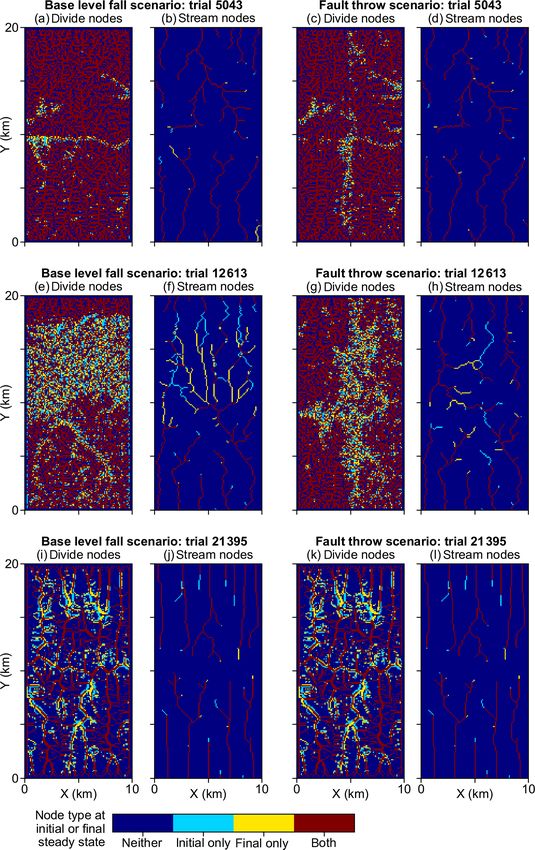
Figure 2. Progression of an experiment trial. The base-level fall and
fault throw scenario trials progressed as outlined in this flowchart. δz
= U − KAm S n + kd ∇ 2 z, (5)
The two phases of the model both included a time loop. The steps in δt
the time loop were repeated until topography reached steady state.
The evolution processes in the time loops are detailed on the right. where U (m yr−1 ) is the rock uplift rate relative to base
Dashed lines connect trial factors to the steps that the factors pa- level, A (m2 ) is contributing drainage area as a surrogate for
rameterise. discharge (for which we used a uniform precipitation rate
of 1 m yr−1 ), S (m m−1 ) is local channel slope, and m and
n were constants in this experiment. Base level in this study
faulting the topography, depending on the scenario. The sim- was the top and bottom boundaries of the model grid. The
ulated landscape and lineages evolved together in this sec- m
erosion coefficient, K (m1−2 yr−1 ), encapsulates surface
ond phase until elevation returned to steady state, at which erodibility, and in real landscapes it is commonly assumed
point the trial ended. In both phases of both scenarios, the to be influenced by rock strength, channel width, channel
time step duration was 1000 years and steady state was de- bed material, and runoff among other variables (Whipple and
fined the same. Steady state was reached when changes in Tucker, 1999).
the mean and standard deviation of elevation over the prior Previously published values of empirically observed up-
1000 time steps (or 1 million model years) was less than 1 %. lift, stream incision, and diffusion parameters guided the se-
A generalised trial is illustrated in Fig. 2. Trial parameters lection of factor intervals that were explored in experiment
are summarised in Table 1 and described in more detail be- trials (Table 1). Regional rock uplift was simulated at each
low. The factor values of each trial are provided in a data time step by uniformly increasing the elevation of all grid
repository associated with this paper (Lyons et al., 2019). nodes except the nodes along the grid boundary, which were
not changed. The magnitude of uplift rate in each trial was
3.2.1 Initial conditions phase set by the “uplift rate” sensitivity analysis factor and varied
generally from orogenic to cratonic values. The maximum
A Landlab raster model grid was initialised with dimensions value of this factor was 1 × 10⁻³ m yr−1 , which is slightly
of 10 km by 20 km and a node spacing of 100 m. The left lower than the rapid uplift rate of 5×10⁻³ m yr−1 reported in
and right boundaries of the grid were closed to mass export, orogenic settings (Burbank et al., 1996; Beavan et al., 2010).
and the top and bottom boundaries were set to open. These The minimum modelled uplift rate of 1 × 10⁻⁵ m yr−1 was
boundary conditions were selected to represent a generic selected because even lower rates led to an impractical com-
landscape drained by streams that dominantly flow to the putation time required to reach steady state in preliminary
north and south separated by a main divide that spanned model runs. The large parameter space explored in model
the width of the grid. The initial topography of each trial trials alleviates complications of selecting more limited pa-
was generated in a two-step process whereby random ele- rameter ranges by bounds that greatly vary globally.
vation noise was first generated, and then topography was
https://doi.org/10.5194/esurf-8-893-2020 Earth Surf. Dynam., 8, 893–912, 2020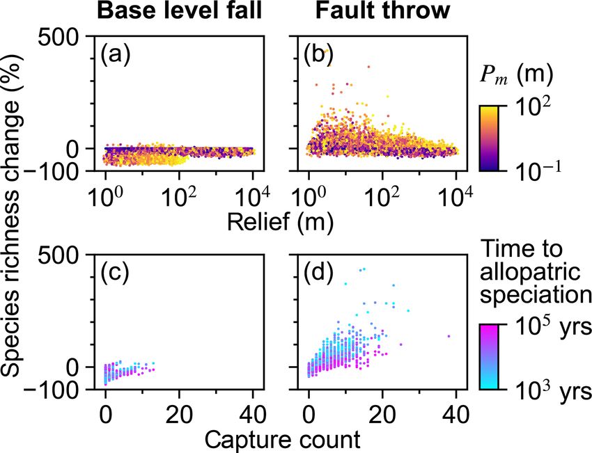
898          N. J. Lyons et al.: Topographic controls on divide migration, stream capture, and diversification in riverine life

   Following uplift in each time step, surface water flow at       Pm spanned values from 0.1 to 100 m. This range falls within
each node was routed in the single direction of the steep-         observed total fault throw (e.g. Roberts and Michetti, 2004),
est descent among the eight adjacent nodes. Stream incision        which is represented by the presence of the fault scarp at
and linear diffusion modified elevation further by the Land-       model onset. At each time step in the perturb phase, the sur-
lab FastscapeEroder and LinearDiffuser components, respec-         face processes were carried out in the same way as in the ini-
tively. Stream power model exponents, m and n, were held           tial condition phase using the same factor values for a given
constant at 0.5 and 1.0, respectively. The factor values for the   trial. The signal of the perturbation through the landscape
stream power model coefficient K ranged from 1.0×10⁻⁶ to           was illustrated using
1.0 × 10⁻⁴ yr−1 . This interval is within reported values of       δx
about 2.5×10⁻⁸ to 2.5×10⁻³ yr−1 (Stock and Montgomery,                = KAm ,                                                   (6)
                                                                   δt
1999; Whipple and Tucker, 1999). The factor values for the
hillslope diffusion coefficient kd ranged from 0.9 × 10⁻⁴ to       where δx δt is the upstream knickpoint migration rate (Berlin
1.0 × 10⁻¹ m2 yr−1 in a review by Martin (2000). We used a         and Anderson, 2007). The maximum Pm value in model trials
smaller range of 1.0 × 10⁻³ to 1.0 × 10⁻¹ m2 yr−1 .                was within the reconstructed rapid base-level fall of 250 m
   Stream networks were identified immediately after the ini-      in the Appalachian Mountains (Prince et al., 2011) and ob-
tial steady state was reached. Grid nodes were designated as       served knickpoint heights, for example the 60 to 110 m range
streams if the node contributing drainage area was greater         of knickpoint heights on the Roan Plateau (Berlin and Ander-
than the value of the sensitivity analysis factor, “critical       son, 2007). Additionally, main divide migration in each trial
drainage area” (Ac ), that varied between 0.5 and 5 km2 in         was calculated by (1) finding the maximum elevation in each
the experiment trials. A discrete stream network is defined        grid column at the first and final time steps of the perturb
here as the streams that share an outlet. Outlets existed only     phase, (2) measuring the distance between the main divide
at the top or bottom boundary of the model grid in the initial     node in the first and final time steps, and (3) averaging the
conditions phase. In the perturb phase described below, net-       distance of the main divide nodes to calculate the mean mi-
works could temporarily exist in internally drained, endoreic      gration of the main divide in the trial.
basins with outlets not on a grid boundary.                           The macroevolutionary processes (i.e. dispersal, speci-
   Each stream network was populated with one species at the       ation, and extinction) ran subsequent to the surface pro-
end of the initial conditions phase. All species were instanti-    cesses in each time step in this application of SpeciesEvolver
ated with the ZoneSpecies class of SpeciesEvolver. The zone        (Fig. 2). A schematised version of Fig. 1 is provided in Fig. 3
of a species was initially set to the stream network wherein       to demonstrate how drainage reorganisation drove species
the species was populated. Species evolved under the de-           evolution in the model of this study. In Fig. 3, adjacent stream
fault ZoneSpecies processes, namely dispersal, speciation,         cells compose a zone of a species. Species dispersal was
and extinction (further described in Sect. 3.2.2), meaning         modelled by resolving the difference in zone extent between
custom-made macroevolutionary processes were not used in           an earlier (T0 ) and later (T1 ) time step. For example, the zone
this study. All species were functionally the same in this ex-     of stream network 5 (N5) expanded by one cell to the north
periment, meaning they behaved similarly when presented            in T1 , and thus the species of this zone (E.0) dispersed to this
with the same landscape conditions. Such functional equiva-        cell between T0 and T1 . If a zone of a species was fragmented
lence (neutrality sensu Hubbell, 2001) can be set differently      (due to stream capture, for example), that species divided
in future research. The processes described in this section        into one or more child species (clades B and H in Fig. 3). A
set the initial conditions of topography, stream networks, and     species became extinct when it was no longer associated with
species for the next phase of the experiment.                      any zones. This occurred when streams in T0 do not overlap
                                                                   any streams in T1 , as exemplified by clade D in Fig. 3.
3.2.2   Perturb phase
                                                                      One parameter of the simulated species varied in the trials
                                                                   of the model experiment. This parameter, “time to allopatric
The steady-state topography was perturbed following the fi-        speciation”, sets a delay from the time step when the zone
nal time step in the initial conditions phase and before the       of a species fragmented to the time step when speciation is
first time step in the perturb phase (Fig. 2). The perturba-       executed by the software. Speciation, when it is triggered by
tion in a base-level fall trial was executed along the bottom      zone fragmentation, is carried out more rapidly as this param-
boundary of the grid on which elevation was decreased by the       eter decreases. The parameter was set to the same value for
value of the perturbation magnitude factor, Pm . The pertur-       all species in a trial, and it varied from 1 to 100 kyr among the
bation in a fault throw trial was executed by a single vertical    trials, consistent with empirical studies on freshwater fishes
fault that instantaneously uplifted the right half of the model    (Albert and Carvalho, 2011; Tedesco et al., 2012; Albert et
grid with a throw equal to the value of Pm . The intent of this    al., 2018) and a theoretical model arising from analyses of
scenario is to demonstrate drainage reorganisation initiated       molecular phylogenies linking speciation to rare stochastic
from a different pattern than base-level decline, rather than      events that cause reproductive isolation (Venditti et al., 2010;
creating a realistic fault growth model (e.g. Cowie, 1998).        Beaulieu and O’Meara, 2015). For example, if the zone of

Earth Surf. Dynam., 8, 893–912, 2020                                                  https://doi.org/10.5194/esurf-8-893-2020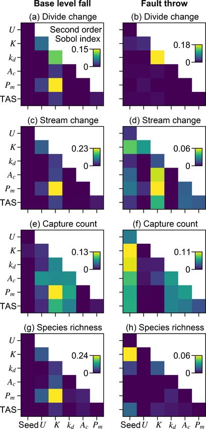
N. J. Lyons et al.: Topographic controls on divide migration, stream capture, and diversification in riverine life                   899

                                                                          3.3    Model response variables

                                                                          The response variables, which are the model outputs inves-
                                                                          tigated in the sensitivity analyses, were collected from each
                                                                          trial. Topographic relief was the only response collected dur-
                                                                          ing the initial conditions phase. It was calculated as the maxi-
                                                                          mum minus the minimum elevation of the grid, excluding the
                                                                          boundary nodes, at the end of the time step when steady state
                                                                          was reached. Four responses that represent drainage reorgan-
                                                                          isation and species lineage diversification were collected at
                                                                          the end of the perturb phase. The “divide percent change
                                                                          response” was calculated by dividing the total cell area of
                                                                          nodes that were drainage divides in either the first or the
                                                                          final time step by the total cell area of nodes that were di-
                                                                          vides in the first and final time steps. Divides were identified
                                                                          where there were no upstream nodes (i.e. node drainage area
                                                                          equalled the cell area). The calculation for “stream percent
                                                                          change response” was similar to the divide percent change
                                                                          response. Streams were identified as the nodes with drainage
                                                                          areas greater than the trial factor value of Ac . Divide and
Figure 3. Downscaled schematic of the modelling approach. (a) A
                                                                          stream change response values were used to characterise the
schematised steady-state landscape wherein the main divide sepa-
                                                                          percent of grid nodes that changed landform type, and these
rates eight stream networks (N1 . . . N8) that each flow to either the
north or south boundary. (b) The species and zones of SpeciesE-           responses are henceforth collectively referred to as “land-
volver are defined at the nodes of a Landlab grid. In this study, nodes   form change”. The “stream capture count response” is the
with a drainage area greater than Ac define the zone of a species.        number of stream captures that occurred during the perturb
(c) The landscape following reorganisation. N6 and N7 captured            phase. A stream capture occurred when stream nodes at a
areas from adjacent networks. While N3 did extend into the water-         time step, t, overlapped the stream nodes of another network
shed of N4, it did not overlap the stream nodes of the prior time         at t − 1. The “species richness percent change response” was
step; therefore, N3 did not capture N4 following the strict definition    calculated as the percent change of species richness between
of capture in this study. N4 disappeared because all nodes in the         the first and final time step of the perturb phase. It was cal-
northeast watershed have a drainage area below the critical drainage      culated as the final minus initial species count divided by the
area. (d) The phylogenetic tree of the species in (a) and (c).
                                                                          initial species count.

a species became fragmented and the trial value of this fac-              4     Results
tor was 1 kyr, speciation occurred in the time step following
fragmentation because the time step duration of the model is              The model responses of the 25 600 trials of each scenario
1 kyr.                                                                    are provided in the data repository associated with this pa-
   The model iterated through time until the time step when               per (Lyons et al., 2019). The “Video supplement” contains
topography returned to steady state at which point the trial              animations (V1–V3) of selected trials that exemplify the to-
ended. This final steady state was defined following the same             pographic response to the single base-level fall or fault throw
conditions as the initial steady state. Steady state was reached          perturbation of a trial. At the onset of a trial perturb phase,
when changes in the mean and standard deviation of eleva-                 steepened hillslopes and stream knickpoints formed where
tion over the prior 1 million model years were less than 1 %.             the perturbation originated, which was at base level along the
In the model designed for this research, evolution effectively            southern model grid boundary or along the fault. Over time,
ceases following drainage stabilisation; this occurs well be-             the steepened landscape portion moved away from the per-
fore the end of the perturb phase, which is when topogra-                 turbation origin, behaving as an erosional wave that locally
phy returns to steady state. However, models using SpeciesE-              steepened topography at the wave front and lowered it in its
volver in future research can readily incorporate evolutionary            wake. The wave separated the upslope landscape portion yet
processes not exclusively driven by landscape structure, for              to adjust to the perturbation from the downslope portion that
example sympatric speciation (Lyons et al., 2020). The land-              has adjusted to the perturbation.
scape and biologic model responses in this research were de-                 The magnitude of the perturbation in the base-level fall
termined from the state of the model immediately following                scenario was a primary control on the migration distance of
the final time step.                                                      the main divide and stream knickpoints. The calculation of
                                                                          the main divide migration distance is described in Sect 3.2.2,
                                                                          and its value for each experiment trial is provided in Lyons

https://doi.org/10.5194/esurf-8-893-2020                                                       Earth Surf. Dynam., 8, 893–912, 2020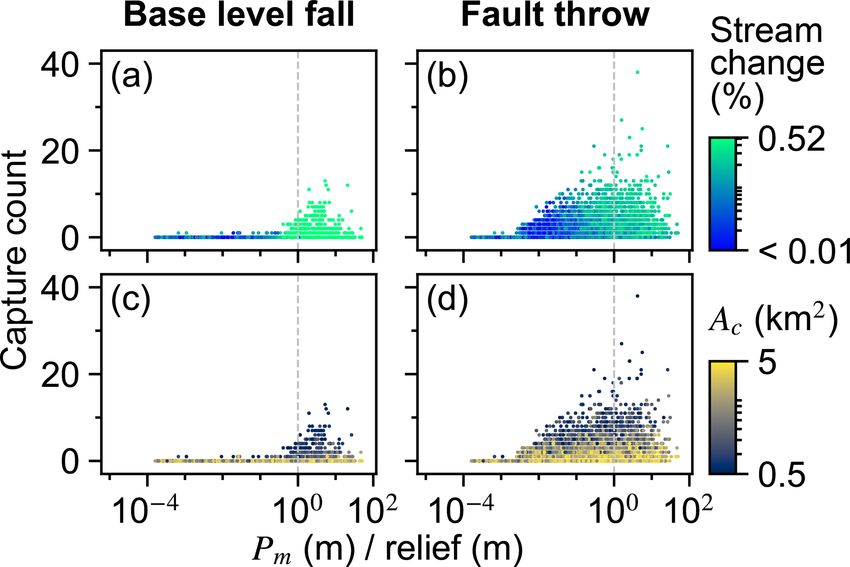
900          N. J. Lyons et al.: Topographic controls on divide migration, stream capture, and diversification in riverine life

et al. (2019). The main divide migrated northward by 250 m
in trial 5043 with a base-level fall of only 2 m (V1). In trials
with a similarly small Pm the wave grew and then decayed,
all in the southern half of the grid, before it reached the main
divide. The main divide was driven northward by 7691 m, al-
most to the northern boundary, following the 72 m base-level
fall in trial 12613 (V2). In both of these exemplary trials,
streams remain fixed in their course while the wave was in
the southern half of the grid. Streams eroded headward once
the wave reached the main divide. The wave propagated at
the velocity predicted by Eq. (6) (V1–V2). The analytically        Figure 4. Histogram of topographic relief. The plotted data repre-
predicted knickpoint locations in the “Video supplement”           sent the topographic relief at the trial end of the initial conditions
                                                                   phase of each trial. Note that the y axis is logarithmic.
animations correspond to the location of knickpoints in the
modelled landscapes at a given time. In a subset of base-level
scenario trials (e.g. trial 3639), not one divide or stream node   tions of the few model trials with relief greater than observed
changed during the experiment (Lyons et al., 2019).                on present-day Earth.
   The animation of a fault throw scenario exemplary trial            The total-order Sobol indices of U and K were the great-
demonstrates a different pattern of erosional wave propa-          est among the factors, indicating relief was most influenced
gation. The wave initiated along the north, west, and south        by U and K (Fig. 5a). U and K individually contributed to
edges of the right block that uplifted instantaneously at the      about half of the variance of relief as indicated by the first-
onset of fault throw scenario trials with high Pm relative to      order indices. The other half – represented by the difference
the experiment range, including the 72 m throw in trial 12613      between the total- and first-order indices of these factors –
(V3 in the “Video supplement”). The waves propagated up            was controlled by second- and higher-order effects. The only
the watersheds of the right upthrown block until the waves         factor pair with a large second-order index was U and K
reached the main divide at about the same time. The main           (Fig. 5b), indicating that relief in a given trial was influenced
divide did not migrate because the base level was the same         by the interaction of these factors, which is expected because
for the networks that drained to the north and south bound-        U and K together set relief as specified in Eq. (6). The out-
aries in this scenario. This behaviour is contrary to the base-    come of this interaction is presented in Fig. 5c. Relief in-
level fall scenario in which the main divide migrated to-          creased with U , and for a given value of U , relief decreased
wards the upper boundary following the elevation decline           with an increase in K.
only along the lower boundary. Drainage reorganisation was            U , K, and Pm were the factors that most influenced divide
concentrated near the horizontal centre of the grid in the         and stream percent change during the perturb phase (Fig. 6a–
fault throw scenario, contrasting with the base-level fall sce-    d). The divide and stream change model responses, collec-
nario in which reorganisation was concentrated in the upper        tively referred to as landform change, indicate the proportion
50 % of the grid. The steeper slope across the fault scarp         that these landforms relocated during trials as described in
redirected streamflow from the upthrown block to the west,         Sect. 3.3. Here we compare the landform change responses
which led to drainage capture by stream networks on the            to steady-state relief, rather than comparing U and K in-
downthrown block in 3 % and 56 % of the base-level fall and        dividually to landform change, because (1) U and K to-
fault throw scenario trials, respectively (Table 2). In a subset   gether predict relief, and (2) the relationship between relief,
of trials, stream segments adjacent to the fault became inter-     Pm , and the landform change responses differed between tri-
nally drained before they connected to a network that drained      als with relief above versus below about 100 m, which coin-
to a grid boundary. Watersheds that did not overlap the fault,     cides with the maximum Pm value. Relief, Pm , and landform
or were not immediately adjacent to watersheds that over-          change increased together in the trials for which relief was
lapped the fault, did not contain networks that reorganised.       less than 100 m (Fig. 7a and b), which was the case in exem-
                                                                   plary trial 5043 for which Pm was 2.03 m. In these trials, the
4.1   Topographic relief and landform change                       change in divide and stream locations was most concentrated
                                                                   near the initial position of the main divide in both scenar-
Topographic relief was calculated once elevation reached           ios and also near the fault trace in the fault throw scenario
steady state in the initial conditions phase of each trial. Re-    (e.g. trial 5043; Fig. 7a–d). Stream tips contracted or ex-
lief varied among the trials, with a maximum trial relief of       panded without capturing segments from adjacent networks
11 055 m (Table 2). Most trials contained low relief relative      (Fig. 8b and d). As Pm increased, for example in exemplary
to the maximum relief in the experiment (Fig. 4) owing to          trial 12613 for which Pm was 72 m and relief was also less
the distribution of model factor values. Relief was less than      than 100 m, the relocation of divides and streams extended to
1000 m in 89 % of trials, and relief was greater than 8000 m       a greater portion of the model grid (Fig. 8e–h).
in only 0.12 % of trials. In Sect. 5.5 we provide considera-

Earth Surf. Dynam., 8, 893–912, 2020                                                   https://doi.org/10.5194/esurf-8-893-2020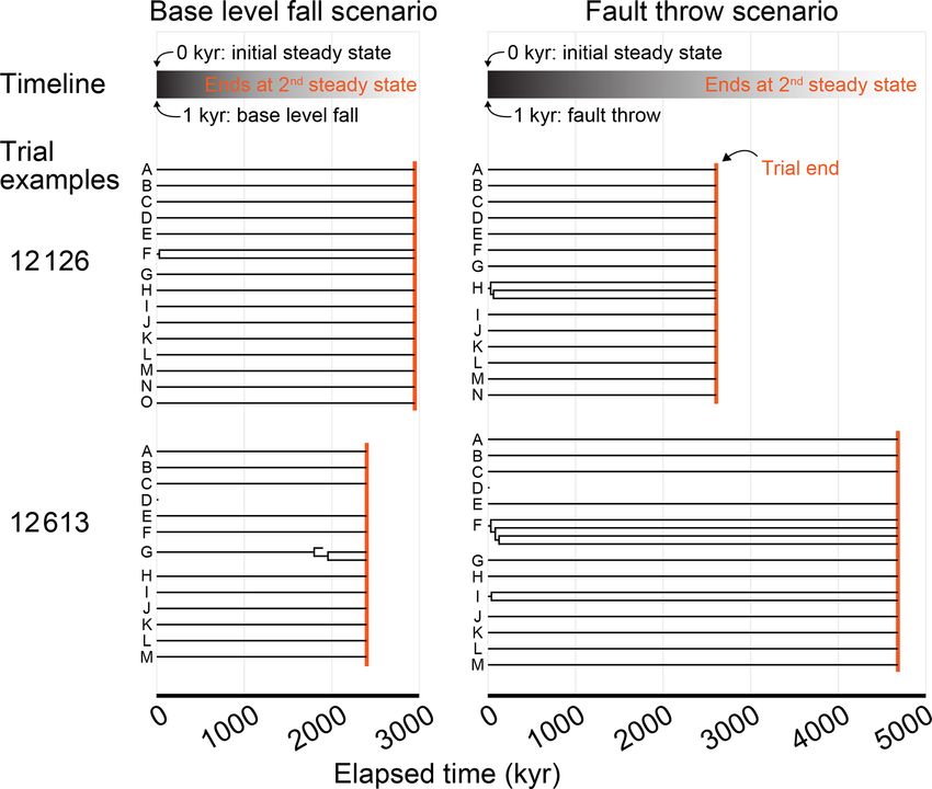
N. J. Lyons et al.: Topographic controls on divide migration, stream capture, and diversification in riverine life                       901

Table 2. Response summary statistics. The perturb-phase statistics are calculated separately for the trials when a given response, R, was
less than, equal to, or greater than 0. Mean values of R were calculated for the trials in which R was not equal to 0. The plus–minus values
associated with the mean R values provide the standard deviation of change for all model trials of a scenario in which R was not equal to 0.

                           Response, R        Statistic                            Initial conditions phase
                           Topographic        minimum                                                         0.9 m
                           relief at steady   mean                                                           447 m
                           state              maximum                                                     11 055 m
                                                                                        Perturb phase
                                                                               Base-level fall          Fault throw
                           Divide percent     trial count: R = 0                   265 (1 %)            173 (1 %)
                           change             trial count: R > 0               25 335 (99 %)        25 427 (99 %)
                                              mean R: R > 0 % change         14.85 ± 13.88 %      11.66 ± 10.12 %
                           Stream percent     trial count: R = 0                  1405 (5 %)           1214 (5 %)
                           change             trial count: R > 0               24 195 (95 %)        24 386 (95 %)
                                              mean R: R > 0 % change         17.99 ± 23.51 %        8.55 ± 7.94 %
                           Capture count      trial count: R = 0               24 919 (97 %)        11 272 (44 %)
                                              trial count: R > 0                   681 (3 %)        14 328 (56 %)
                                              mean R: R > 0 captures             2.35 ± 2.11          2.44 ± 2.14
                           Species            trial count: R < 0             10 135 (39.6 %)       5380 (21.0 %)
                           percent change     trial count: R = 0             15 412 (60.2 %)      10 140 (39.6 %)
                           richness           trial count: R > 0                  53 (0.2 %)      10 080 (39.4 %)
                                              R mean: R < 0 % change       −25.06 ± 19.67 %      −12.27 ± 5.61 %
                                              R mean: R > 0 % change         10.93 ± 4.56 %      21.73 ± 21.59 %

Figure 5. Sobol indices of topographic relief. (a) The first- and total-order Sobol indices of relief at the initial steady state. Model input
factors are on the x axis; “seed” is the initial elevation seed. (b) Second-order Sobol indices of relief. Factors are on the x and y axes.
(c) Relief versus U and K. Each point represents one of the unique steady-state landscapes created in the initial conditions phase.

   The change in the position of streams and divides in the              changed location during the perturb phase reached only about
base-level fall scenario was concentrated near the initial po-           30 % when relief was less than 100 m, except in the few
sition of the main divide in the trials for which divides and            trials in which (1) kd was near the experiment maximum
streams were mobile. In the trials in which Pm was greater               of 10−1 m2 yr−1 and (2) relief approached 100 m (Fig. 7b).
than relief, streams and divides relocated throughout the                Maximum landform change was lower in this scenario be-
northern half of the grid as the main divide drove further               cause topography was primarily perturbed in catchments
northward (e.g. trial 12613; Fig. 8e and f; V2 in the “Video             near the fault compared to the base-level fall scenario in
supplement”). South-flowing streams extended almost to the               which a greater proportion of landforms changed in the wake
northern boundary and tended to reoccupy channels initially              of the erosional wave that spanned the width of the grid. For
incised by north-flowing streams (Fig. 8f). Up to about 80 %             this reason, the Pm total-order index of divide change was
of stream nodes were changed when relief was less than                   relatively lower in the fault throw scenario (Fig. 6a and b). In
100 m in this scenario (Fig. 7e).                                        trials with a relatively large Pm , for example the 72 m fault
   Landform change in the fault throw scenario was concen-               slip in exemplary trial 12613 compared with the 2.03 m slip
trated near the fault trace. The percentage of divides that              in trial 5043, divide and stream relocation was concentrated

https://doi.org/10.5194/esurf-8-893-2020                                                         Earth Surf. Dynam., 8, 893–912, 2020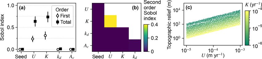
902           N. J. Lyons et al.: Topographic controls on divide migration, stream capture, and diversification in riverine life

                                                                      Figure 7. Landform change responses versus initial relief. Re-
                                                                      sponses of all trials for divide percent change (a–d) and stream per-
Figure 6. First- and total-order Sobol indices of drainage reorgan-   cent change (e, f). The labelled points are the IDs of the exemplary
isation responses. The factors are along the x axis for each of the   trials depicted in Fig. 8 and described in the text.
responses (a–h); “seed” refers to the initial elevation seed.

                                                                      changed in response to the combined values of multiple fac-
around the fault (Fig. 8g and h), and the influence of kd on          tors (Fig. 9d), they changed mostly along with K. The total
divide change became relatively greater than strictly Pm as           effect of kd for stream change was also lower in both sce-
described below. In both scenarios, a greater Pm produced             narios. Stream change was minimally affected by kd because
a steeper erosion front that propagated further and disrupted         diffusion minimally affects channels (Fig. 8j and l).
drainages in its passage. The relatively higher second-order
Sobol index of factor pair K and Pm in most of the landform           4.2   Controls on stream capture occurrence
change responses (Fig. 9a, c and d) indicates the relative im-
portance of the interactions among these factors.                     The frequency and grid location of stream captures differed
   Divide change increased with kd when relief was greater            between the two scenarios. Captures occurred in 3 % and
than 100 m in both scenarios (Fig. 7c and d). The increase            56 % of the trials in the base-level fall and fault throw sce-
in kd with divide change at greater relief, combined with the         narios, respectively (Table 2). Captures in the trials of the
low range of divide change at low relief in the fault throw           base-level fall scenario tended to be located in one of two
scenario, elevated the importance of kd to this response in           grid areas. Near the main divide once the erosional wave
this scenario (Fig. 6a and b). In both scenarios, divide change       reached this divide, a stream of a southern network captured
reached about 40 % in trials in which relief was near 100 m           a segment of a northern network as the erosional wave drove
and kd was near the experiment maximum of 10−1 m2 yr−1                northward expansion of the southern networks (V2 in the
(Fig. 7c and d). In these trials, the stream networks and area        “Video supplement”). Captures in this scenario also tended
of catchments tended to not change substantially, although            to be located near the lower boundary when nearby streams
many divides shifted less than 500 m (e.g. trial 21395; Fig. 8i       were diverted to different outlets following base-level fall
and k). Trial 21395 is within the area in Fig. 7c and d where         (e.g. trial 12126; V4).
kd increased with divide change. This area corresponds to the            Streams were captured across the fault trace in the fault
trials in which K is less than 2×10⁻⁶ yr−1 , the values nearest       throw scenario. In many trials, closed basins (i.e. endorheic)
to the experiment minimum of this factor.                             were formed along the fault and were involved in stream
   The relative influence of the factors on stream change was         capture. First, stream segments detached from the initial net-
similar to divide change with a few exceptions (Fig. 6a–d).           works where the instantaneous fault slip formed a scarp that
The total effect of the initial elevation seed was relatively         blocked streamflow and formed closed basins (V3). Over
greater for stream change in the fault throw scenario. The            time these basins and the stream segments within them con-
total-order effect of K was lower for stream change than di-          tinued to uplift and erode as the local relief declined. The
vide change in the fault throw scenario. Although streams             detached segment within the closed basin was captured by a

Earth Surf. Dynam., 8, 893–912, 2020                                                      https://doi.org/10.5194/esurf-8-893-2020
N. J. Lyons et al.: Topographic controls on divide migration, stream capture, and diversification in riverine life 903 Figure 8. Landform change in exemplary trials. This figure illustrates landform change model responses of the trials discussed in Sect. 4 and labelled in Fig. 7. The colour of grid cells symbolises landform type at the initial and final steady state in the model. Blue areas were not the landform type (divide or stream) in a given subplot at the times of either steady state. Red areas were the subplot landform type in both steady-state times. Cyan and yellow areas were the subplot landform type in the initial and final steady state, respectively. The parameter values of these trials and all other trials are provided in Lyons et al. (2019). https://doi.org/10.5194/esurf-8-893-2020 Earth Surf. Dynam., 8, 893–912, 2020
904           N. J. Lyons et al.: Topographic controls on divide migration, stream capture, and diversification in riverine life

                                                                        Figure 10. Capture count versus the ratio of Pm and relief. Pm and
                                                                        relief are equal at the vertical dashed line.

                                                                        networks was important only in the fault throw scenario be-
                                                                        cause only the networks near the fault were perturbed.
                                                                           Multiple other factors contributed to the number of cap-
                                                                        tures in the trials of both scenarios (Fig. 6e and f). Factors U ,
                                                                        K, Pm , and Ac were similarly important within a given sce-
                                                                        nario. Confidence intervals of factors were large in the base-
                                                                        level fall scenario in which captures occurred in relatively
                                                                        few trials. Nevertheless, the interaction of Pm and K was
                                                                        elevated above other interactions in this scenario (Fig. 9e).
                                                                        We examined capture count versus the ratio of Pm and re-
                                                                        lief, as the result of U and K, given the control that these
                                                                        factors acted together to influence landform change. Streams
                                                                        more readily changed location and the number of captures in-
                                                                        creased rapidly in the trials for which Pm : relief exceeded 1
                                                                        (Fig. 10a and b). In trials well below this value, captures were
                                                                        fewer and stream change was limited to minor expansion and
                                                                        contraction of stream tips (e.g. trial 5043; Fig. 8b and d).
                                                                        Multiple captures did occur when Pm : relief was slightly less
Figure 9. Second-order Sobol indices. Second-order indices of
                                                                        than 1 in numerous trials of the fault throw scenario (Fig. 10b
paired model factors for the perturb-phase responses. A relatively
large value in a subplot indicates that the interaction of the factor   and d). The stream networks fragmented in these trials, form-
pair affects the response more than other factor pairs with lower       ing endorheic basins that existed for a few time steps, and
index values.                                                           then the network segments reconnected to a configuration
                                                                        similar to the pre-perturbation configuration. This reorgani-
                                                                        sation sequence incremented capture count as the fragmented
                                                                        network segments reintegrated.
stream that breached the closed basin, and hillslopes within               Ac contributed to the variation in capture count among the
the basin were soon dissected again. In a few trials, captures          trials (Fig. 6e and f). Capture count increased with decreas-
also occurred where the upper stream reaches of networks                ing Ac (Fig. 10c and d). This relationship is most apparent
on the upthrown block were captured by a network on the                 where Pm : relief is near 1 because this ratio value was also
downthrown block.                                                       required for capture count to increase. Few captures occurred
   The initial elevation seed factor had the greatest total-order       even when Ac was near the experiment minimum of this fac-
effect and interacted with many factors to influence cap-               tor in trials for which Pm : relief was well below 1.
ture occurrence in the fault throw scenario (Figs. 6f and 9f).
Stream networks emerged during the initial conditions phase             4.3   Controls on species richness
from the randomly generated elevation noise at the onset of a
model trial. The noise was set by the value of the seed that led        The relationships among relief, Pm , and species richness
to the initial stream networks. The initial location of stream          change differed between the scenarios. Species richness in-

Earth Surf. Dynam., 8, 893–912, 2020                                                         https://doi.org/10.5194/esurf-8-893-2020
N. J. Lyons et al.: Topographic controls on divide migration, stream capture, and diversification in riverine life 905
Figure 11. Species richness percent change. Species richness
change versus relief (a, b) and capture count (c, d).
Figure 12. Phylogeny of exemplary trials. Topography was per-
turbed by base-level fall of fault throw at 1 kyr elapsed since the first
steady state was reached. Most of the trials animated in the “Video
creased in 0.2 % and 39.4 % of trials of the base-level fall supplement” are shown. Trial 5043 is not included. Species did not
and fault throw scenario, respectively (Table 2). Species rich- change in this trial because no stream networks disappeared or were
ness did not change or decreased in the majority of the base- captured. The lineages of clades in a trial are labelled alphabeti-
level fall trials (Table 2; Fig. 11a). A decrease in richness cally. Speciation events occurred when lineages split and extinction
occurred when the final species count was less than the ini- occurred when lineages terminated before the end of the trial.
tial count, meaning extinction was more common than spe-
ciation. Extinction in this simple implementation of Specie-
sEvolver occurred only when all of the stream networks of throw scenario in which the initial elevation seed and kd to-
a species disappeared. A network disappeared when its min- tal effect indices were comparably greater. The relative mag-
imum drainage area decreased below Ac . Species richness nitudes of species-richness-change Sobol indices were more
decreased up to 78 % when topographic relief was less than similar to capture count than landform change responses in
100 m in a trial (Fig. 11a). Below about 100 m of relief, in- the fault throw scenario (Figs. 6h and 9h).
creasingly greater Pm was required for a loss in species rich- The timeframe of speciation following a perturbation dif-
ness. In the fault throw scenario, a greater increase in species fered among the trials. This is exemplified in the trials an-
richness occurred in a subset of trials with low relief and even imated in the “Video supplement” and the phylogeny of
moderate Pm . their simulated species (Fig. 12). Speciation and extinction
Stream capture count and species richness increased to- ceased soon after the perturbation in exemplary trial 12126
gether with wide variability (Fig. 11c and d). Trials in the of both scenarios and trial 12613 of the fault throw sce-
base-level fall scenario with relatively little time to allopatric nario. Speciation and extinction continued to near the end of
speciation increased with capture count and species richness trial 12613 in the base-level fall scenario in which captures
change. Overall, the relationship of time to allopatric speci- did not occur until the erosional wave reached the main di-
ation with capture count and species richness change is un- vide (V5 in the “Video supplement”). The lineage of clade F
clear given the relatively few trials with captures in this sce- in trial 12613 of the fault throw scenario became most di-
nario. In the fault throw scenario, species richness increased verse with four species, whereby two stream networks were
as the time to allopatric speciation decreased for a given cap- captured by a third network soon after the perturbation (V6).
ture count. Clade D in both scenarios of trial 12613 went extinct in the
The relative influence of factors on species richness dif- time step following the perturbation.
fered between the scenarios more than the other responses
(Fig. 6). U , K, and Pm were the factors with the greatest
5 Discussion
total-order indices of species richness percent change in the
base-level fall scenario. Additionally, the relative magnitudes 5.1 Are landscapes with low or high topographic relief
of the species-richness-change Sobol indices were more sim- more susceptible to drainage reorganisation?
ilar to the landform change responses than capture count in
this scenario (Figs. 6g and 9g). The relative importance of Pm The ratio of the relative value of trial Pm to steady-state relief
to species richness change was comparably lower in the fault was a primary control on the degree of drainage reorganisa-
https://doi.org/10.5194/esurf-8-893-2020 Earth Surf. Dynam., 8, 893–912, 2020You can also read


