Estimates of lightning NOx production based on high-resolution OMI NO2 retrievals over the continental US
←
→
Page content transcription
If your browser does not render page correctly, please read the page content below
Atmos. Meas. Tech., 13, 1709–1734, 2020
https://doi.org/10.5194/amt-13-1709-2020
© Author(s) 2020. This work is distributed under
the Creative Commons Attribution 4.0 License.

Estimates of lightning NOx production based on high-resolution
OMI NO2 retrievals over the continental US
Xin Zhang1,2 , Yan Yin1,2 , Ronald van der A2,3 , Jeff L. Lapierre4 , Qian Chen1,2 , Xiang Kuang1,2 , Shuqi Yan2 ,
Jinghua Chen1,2 , Chuan He1,2 , and Rulin Shi1,2
1 CollaborativeInnovation Center on Forecast and Evaluation of Meteorological Disasters/Key Laboratory for
Aerosol-Cloud-Precipitation of China Meteorological Administration, Nanjing University of Information Science and
Technology (NUIST), Nanjing 210044, China
2 Department of Atmospheric Physics, Nanjing University of Information Science and Technology (NUIST),

Nanjing 210044, China
3 Royal Netherlands Meteorological Institute (KNMI), Department of Satellite Observations, De Bilt, the Netherlands
4 Earth Networks, Germantown, Maryland, USA

Correspondence: Yan Yin (yinyan@nuist.edu.cn)

Received: 2 October 2019 – Discussion started: 27 November 2019
Revised: 8 March 2020 – Accepted: 11 March 2020 – Published: 7 April 2020

Abstract. Lightning serves as the dominant source of ni-             needed, given its large influence on the estimation of LNO2
trogen oxides (NOx =NO + NO2 ) in the upper troposphere              PE.
(UT), with a strong impact on ozone chemistry and the
hydroxyl radical production. However, the production ef-
ficiency (PE) of lightning nitrogen oxides (LNOx ) is still
quite uncertain (32–1100 mol NO per flash). Satellite mea-           1   Introduction
surements are a powerful tool to estimate LNOx directly
compared to conventional platforms. To apply satellite data          Nitrogen oxides (NOx ) near the Earth’s surface are mainly
in both clean and polluted regions, a new algorithm for cal-         produced by soil, biomass burning, and fossil fuel combus-
culating LNOx has been developed that uses the Berkeley              tion, while NOx in the middle and upper troposphere orig-
High-Resolution (BEHR) v3.0B NO2 retrieval algorithm and             inates largely from lightning and aircraft emissions. NOx
the Weather Research and Forecasting model coupled with              plays an important role in the production of ozone (O3 ) and
chemistry (WRF-Chem). LNOx PE over the continental US                the hydroxyl radical (OH). While the anthropogenic sources
is estimated using the NO2 product of the Ozone Monitor-             of NOx are largely known, lightning nitrogen oxides (LNOx )
ing Instrument (OMI) data and the Earth Networks Total               are still the source with the greatest uncertainty, though they
Lightning Network (ENTLN) data. Focusing on the sum-                 are estimated to range between 2 and 8 Tg N yr−1 (Schu-
mer season during 2014, we find that the lightning NO2               mann and Huntrieser, 2007). LNOx is produced in the up-
(LNO2 ) PE is 32 ± 15 mol NO2 per flash and 6 ± 3 mol NO2            per troposphere (UT) by O2 and N2 dissociation in the hot
per stroke while LNOx PE is 90 ± 50 mol NOx per flash and            lightning channel as described by the Zel’dovich mechanism
17 ± 10 mol NOx per stroke. Results reveal that our method           (Zel’dovich and Raizer, 1967). With the recent updates of
reduces the sensitivity to the background NO2 and includes           UT NOx chemistry, the daytime lifetime of UT NOx is eval-
much of the below-cloud LNO2 . As the LNOx parameteriza-             uated to be ∼ 3 h near thunderstorms and ∼ 0.5–1.5 d away
tion varies in studies, the sensitivity of our calculations to the   from thunderstorms (Nault et al., 2016, 2017). This results
setting of the amount of lightning NO (LNO) is evaluated.            in enhanced O3 production in the cloud outflow of active
Careful consideration of the ratio of LNO2 to NO2 is also            convection (Pickering et al., 1996; Hauglustaine et al., 2001;
                                                                     DeCaria et al., 2005; Ott et al., 2007; Dobber et al., 2008;
                                                                     Allen et al., 2010; Finney et al., 2016). As O3 is known as

Published by Copernicus Publications on behalf of the European Geosciences Union.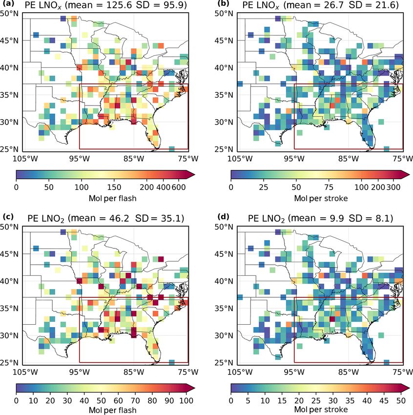
1710                                                                 X. Zhang et al.: Estimates of lightning NOx production

a greenhouse gas, strong oxidant, and absorber of ultraviolet      eled by Tracer Model 3 (TM3). Martin et al. (2007) analyzed
radiation (Myhre et al., 2013), the contributions of LNOx to       SCIAMACHY NO2 columns with Goddard Earth Observing
O3 production also have an effect on climate forcing. Finney       System chemistry model (GEOS-Chem) simulations to iden-
et al. (2018) found different impacts on atmospheric compo-        tify LNOx production amounting to 6 ± 2 Tg N yr−1 .
sition and radiative forcing when simulating future lightning         As these methods focus on monthly or annual mean NO2
using a new upward cloud ice flux (IFLUX) method versus            column densities, more recent studies applied specific ap-
the commonly used cloud-top height (CTH) approach. While           proaches to investigate LNOx directly over active convec-
global lightning is predicted to increase by 5 %–16 % over         tion. Beirle et al. (2006) estimated LNOx as 1.7 (0.6–
the next century with the CTH approach (Clark et al., 2017;        4.7) Tg N yr−1 based on a convective system over the Gulf
Banerjee et al., 2014; Krause et al., 2014), a 15 % decrease       of Mexico, using National Lightning Detection Network
in global lightning was estimated with IFLUX in 2100 under         (NLDN) observations and GOME NO2 column densities.
a strong global warming scenario (Finney et al., 2018). As a       However, it is assumed that all the enhanced NO2 originated
result of the different effects on radiative forcing from ozone    from lightning and did not consider the contribution of an-
and methane, a net positive radiative forcing was found with       thropogenic emissions. Beirle et al. (2010) analyzed LNOx
the CTH approach while there is little net radiative forcing       production systematically using the global dataset of SCIA-
with the IFLUX approach (Finney et al., 2018). However, the        MACHY NO2 observations combined with flash data from
convective available potential energy (CAPE) times the pre-        the World Wide Lightning Location Network (WWLLN).
cipitation rate (P ) proxy predicts a 12 ± 5 % increase in the     Their analysis was restricted to 30 km × 60 km satellite pix-
continental US (CONUS) lightning strike rate per kelvin of         els where the flash rate exceeded 1 flash km−2 h−1 . But they
global warming (Romps et al., 2014), while the IFLUX proxy         found LNOx production to be highly variable, and correla-
predicts the lightning will only increase 3.4 % K−1 over the       tions between flash-rate densities and LNOx production were
CONUS. Recently, Romps (2019) compared the CAPE ×P                 low in some cases. Bucsela et al. (2010) estimated LNOx
proxy and IFLUX method in cloud-resolving models. They             production as ∼ 100–250 mol NOx per flash for four cases,
reported that higher CAPE and updraft velocities caused by         using the DC-8 and OMI data during NASA’s Tropical Com-
global warming could lead to the large increases in tropi-         position, Cloud and Climate Coupling Experiment (TC4).
cal lightning simulated by the CAPE ×P proxy, while the               Based on the approach used by Bucsela et al. (2010), a
IFLUX proxy predicts little change in tropical lightning be-       special algorithm was developed by Pickering et al. (2016)
cause of the small changes in the mass flux of ice.                to retrieve LNOx from OMI and the WWLLN. The al-
   In view of the regionally dependent lifetime of NOx and         gorithm takes the OMI tropospheric slant column density
the difficulty of measuring LNOx directly, a better under-         (SCD) of NO2 (SNO2 ) as the tropospheric slant column den-
standing of the LNOx production is required, especially            sity of LNO2 (SLNO2 ) by using cloud radiance fraction (CRF)
in the tropical and midlatitude regions in summer. Using           greater than 0.9 to minimize or screen the lower tropospheric
its distinct spectral absorption lines in the near-ultraviolet     background. To convert the SLNO2 to the tropospheric ver-
(UV) and visible (VIS) ranges (Platt and Perner, 1983), NO2        tical column density (VCD) of LNOx (VLNOx ), an air mass
can be measured by satellite instruments like the Global           factor (AMF) is calculated by dividing the a priori SLNO2 by
Ozone Monitoring Experiment (GOME; Burrows et al.,                 the a priori VLNOx . The a priori SLNO2 is calculated using a
1999; Richter et al., 2005), SCanning Imaging Absorp-              radiative transfer model and a profile of LNO2 simulated by
tion SpectroMeter for Atmospheric CHartographY (SCIA-              the NASA Global Modeling Initiative (GMI) chemical trans-
MACHY; Bovensmann et al., 1999), the Second Global                 port model. The a priori VLNOx is also obtained from the
Ozone Monitoring Experiment (GOME-2; Callies et al.,               GMI model. Results for the Gulf of Mexico during 2007–
2000), and the Ozone Monitoring Instrument (OMI; Levelt            2011 summer yield LNOx production of 80±45 mol NOx per
et al., 2006). OMI has the highest spatial resolution, least in-   flash. Since they considered NO2 above the cloud to be LNO2
strument degradation, and longest record among these satel-        in the algorithm due to the difficulty and uncertainty in de-
lites (Krotkov et al., 2017). Satellite measurements of NO2        termining the background NO2 , their AMF and derived VCD
are a powerful tool compared to conventional platforms be-         of LNOx (LNO2 ) are named AMFLNOx Clean (AMFLNO2 Clean )
cause of their global coverage, constant instrument features,      and LNOx Clean (LNO2 Clean), respectively. Note that Pick-
and temporal continuity.                                           ering et al. (2016) considered the two estimates of back-
   Recent studies have determined and quantified LNOx us-          ground derived from aircraft flights in the Gulf of Mexico
ing satellite observations. Beirle et al. (2004) constrained the   region (3 % and 33 %) and subtracted the mean value (18 %)
LNOx production to 2.8 (0.8–14) Tg N yr−1 by combining             from the estimated mean LNOx production efficiency (PE)
GOME NO2 data and flash counts from the Lightning Imag-            for the background bias. However, we use the original algo-
ing Sensor (LIS) aboard the Tropical Rainfall Measurement          rithm directly without correction to distinguish the effect of
Mission (TRMM) over Australia. Boersma et al. (2005) esti-         different AMFs on LNOx estimation in the remainder of this
mated the global LNOx production of 1.1–6.4 Tg N yr−1 by           paper. Unless otherwise specified, abbreviations S and V are
comparing GOME NO2 with distributions of LNO2 mod-

Atmos. Meas. Tech., 13, 1709–1734, 2020                                             www.atmos-meas-tech.net/13/1709/2020/
X. Zhang et al.: Estimates of lightning NOx production                                                                      1711

respectively defined as the tropospheric SCD and VCD in           the bias of AMF related to these observations is reduced to
this paper.                                                       < ±4 % for OMI viewing geometries.
   More recently Bucsela et al. (2019) obtained an average           In this paper, we focus on the estimation of LNO2 produc-
PE of 180 ± 100 mol NOx per flash over East Asia, Europe,         tion per flash (LNO2 per flash), LNOx production per flash
and North America based on a modification of the method           (LNOx per flash), LNO2 production per stroke (LNO2 per
used in Pickering et al. (2016). A power function between         stroke), and LNOx production per stroke (LNOx per stroke)
LNOx and lightning flash rate was established, while the          in May–August (MJJA) 2014 by developing an algorithm
minimum flash-rate threshold was not applied. The tropo-          similar to that of Pickering et al. (2016) based on the BEHR
spheric NOx background was removed by subtracting the             NO2 retrieval algorithm (Laughner et al., 2018, 2019), but it
temporal average of NOx at each box where the value was           performs better over background NO2 sources. Section 2 de-
weighted by the number of OMI pixels which meet the op-           scribes the satellite data, lightning data, model settings, and
tical cloud pressure and CRF criteria required to be consid-      the algorithm in detail. Section 3 explores the suitable data
ered deep convection but have one flash or fewer instead. The     criteria, compares different methods, and evaluates the effect
lofted pollution was considered to be 15 % of total NOx ac-       of background NO2 , cloud, and LNOx parameterization on
cording to the estimation from DeCaria et al. (2000, 2005),       LNOx production estimation. Section 4 examines the effect
and the average chemical delay was adjusted by 15 % follow-       of different sources of the uncertainty on the results. Conclu-
ing the 3 h LNOx lifetime in the nearby field of convection       sions are summarized in Sect. 5.
(Nault et al., 2017). However, there were negative LNOx val-
ues caused by the overestimation of the tropospheric back-
ground and stratospheric NO2 at some locations.                   2     Data and methods
   On the other hand, Lapierre et al. (2020) constrained
                                                                  2.1    Ozone Monitoring Instrument (OMI)
LNO2 to 1.1 ± 0.2 mol NO2 per stroke for intracloud (IC)
strokes and 10.7 ± 2.5 mol NO2 per stroke for cloud-to-           OMI is carried on the Aura satellite (launched in 2004), a
ground (CG) strokes over the CONUS. LNO2 per stroke               member of the A-train satellite group (Levelt et al., 2006,
was scaled to 24.2 mol NOx per flash using mean values of         2018). OMI passes over the Equator at ∼ 13:45 LT (ascend-
strokes per flash and the ratio of NOx to NO2 in the UT.          ing node) and has a swath width of 2600 km, with a nadir
They used the regridded Berkeley High-Resolution (BEHR)           field-of-view resolution of 13 km × 24 km. Since the begin-
v3.0A 0.05◦ × 0.05◦ “visible only” NO2 VCD (Vvis ) product        ning of 2007, some of the measurements have become use-
which includes two parts of NO2 that can be “seen” by the         less as a result of anomalous radiances called the “row
satellite. The first part is the NO2 above clouds (pixels with    anomaly” (Dobber et al., 2008; KNMI, 2012). For the current
CRF > 0.9) and the second part is the NO2 detected from           study, we used the NASA standard product v3.0 (Krotkov
cloud-free areas. A threshold of 3×10¹⁵ molecules cm−2 , the      et al., 2017) as input to the LNOx retrieval algorithm.
typical urban NO2 concentration, was applied to mask the             The main steps of calculating the NO2 tropospheric VCD
contaminated grid cells (Beirle et al., 2010; Laughner and        (VNO2 ) in the NASA product include the following.
Cohen, 2017). The main difference between Lapierre et al.
(2020) and Pickering et al. (2016) is the air mass factor for         1. SCDs are determined by the OMI-optimized differential
lightning (AMFLNOx ) implemented in the basic algorithm. In              optical absorption spectroscopy (DOAS) spectral fit.
Lapierre et al. (2020), the air mass factor was used to convert       2. A corrected (“de-striped”) SCD is obtained by subtract-
SNO2 to Vvis , while in Pickering et al. (2016) it was used to           ing the cross-track bias caused by an instrument artifact
convert SLNO2 to VLNOx , assuming that all SNO2 is generated             from the measured slant column.
by lightning.
   To apply the approach used by Bucsela et al. (2010), Pick-         3. The AMF for stratospheric (AMFstrat ) or tropospheric
ering et al. (2016), Bucsela et al. (2019), and Lapierre et al.          column (AMFtrop ) is calculated from the NO2 profiles
(2020) without geographic restrictions, the contamination by             integrated vertically using weighted scattering weights
anthropogenic emissions must be taken into account in de-                with the a priori profiles. These profiles are obtained
tail. The Weather Research and Forecasting (WRF) model                   from GMI monthly mean profiles using 4 years (2004–
coupled with chemistry (WRF-Chem) has been employed                      2007) of simulation.
to evaluate the convective transport and chemistry in many
                                                                      4. The stratospheric NO2 VCD (Vstrat ) is calculated from
studies (Barth et al., 2012; Wong et al., 2013; Fried et al.,
                                                                         the subtraction of the a priori contribution from tropo-
2016; Li et al., 2017). Meanwhile, Laughner and Cohen
                                                                         spheric NO2 and a three-step (interpolation, filtering,
(2017) showed that the OMI AMF is increased by ∼ 35 %
                                                                         and smoothing) algorithm (Bucsela et al., 2013).
for summertime when LNO2 simulated by WRF-Chem is
included in the a priori profiles to match aircraft observa-          5. Vstrat is converted to the slant column using AMFstrat
tions. The simulation agrees with observed NO2 profiles and              and subtracted from the measured SCDs to yield SNO2 ,
                                                                         leading to VNO2 = SNO2 /AMFtrop .

www.atmos-meas-tech.net/13/1709/2020/                                                Atmos. Meas. Tech., 13, 1709–1734, 2020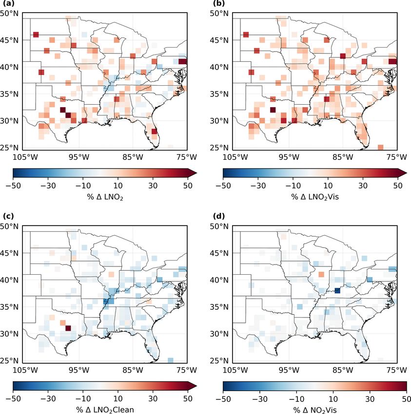
1712                                                                X. Zhang et al.: Estimates of lightning NOx production

      Based on this method, we developed a new AMFLNOx
      to obtain the desired VLNOx (VLNOx = SNO2 /AMFLNOx )
      by replacing the original step.
 6. Details of this algorithm are discussed in Sect. 2.4.

2.2    The Earth Networks Total Lightning Detection
       Network (ENTLN)

The Earth Networks Total Lightning Network (ENTLN) op-
erates a system of over 1500 ground-based stations around
the world with more than 900 sensors installed in the
CONUS (Zhu et al., 2017). Both IC and CG lightning flashes
are located by the sensors with detection frequency ranging
from 1 Hz to 12 MHz based on the electric field pulse polar-      Figure 1. Domain and terrain height (m) of the WRF-Chem simula-
ity and wave shapes. Groups of pulses are classified as a flash   tion with 350 × 290 grid cells and a horizontal resolution of 12 km.
if they are within 700 ms and 10 km. In the preprocessed data
obtained from the ENTLN, both strokes and lightning flashes       level of neutral buoyancy parameterization (Price and Rind,
composed of one or more strokes are included.                     1992; Wong et al., 2013) and LNOx parameterizations is ac-
    Rudlosky (2015) compared ENTLN combined events (IC            tivated (200 mol NO per flash, the factor to adjust the pre-
and CG) with LIS flashes and found that the relative flash        dicted number of flashes is set to 1, hereinafter referred to as
detection efficiency of ENTLN over CONUS increases from           “1 × 200 mol NO per flash”). Simulated total flash densities
62.4 % during 2011 to 79.7 % during 2013. Lapierre et al.         are higher than ENTLN observations over the southeast US
(2020) also compared combined ENTLN and the NLDN                  and lower than observations in the north-central US (Fig. 2).
dataset with data from the LIS during 2014 and found the          The impact of these biases on LNOx production is discussed
detection efficiencies of IC flashes and strokes to be 88 %       and mitigated in Sect. 3.1 and 3.4. The bimodal profile mod-
and 45 %, respectively. Since we only use the ENTLN data          ified from the standard Ott et al. (2010) profile (Laughner
in 2014 as Lapierre et al. (2020), and NLDN detection ef-         and Cohen, 2017) is employed as the vertical distribution of
ficiency of IC pulses should be lower than 33 %, which is         lightning NO (LNO) in WRF-Chem, while outputs of LNO
calculated by the data in 2016 (Zhu et al., 2016), only the IC    and LNO2 profiles are defined as the difference of vertical
flashes and strokes are divided by 0.88 and 0.45, respectively,   profiles between simulations with and without lightning.
while CG flashes and strokes are unchanged because of the
high detection efficiency.                                        2.4   Method for deriving AMF

2.3    Model description                                          The VLNOx near convection is calculated according to

The present study uses WRF-Chem version 3.5.1 (Grell                          SNO2
                                                                  VLNOx =            ,                                            (1)
et al., 2005) with a horizontal grid size of 12 km × 12 km                   AMFLNOx
and 29 vertical levels (Fig. 1). The initial and boundary con-
                                                                  where SNO2 is the OMI-measured tropospheric slant column
ditions of meteorological parameters are provided by the
                                                                  NO2 , and AMFLNOx is a customized lightning air mass fac-
North American Regional Reanalysis (NARR) dataset with
                                                                  tor. The concept of AMFLNOx was also used in Beirle et al.
a 3-hourly time resolution. Based on Laughner et al. (2019),
                                                                  (2009) to investigate the sensitivity of satellite instruments to
3D wind fields, temperature, and water vapor are nudged to-
                                                                  freshly produced lightning NOx . In order to estimate LNOx ,
wards the NARR data. Outputs from version 4 of the Model
                                                                  we define the AMFLNOx as the ratio of the “visible” modeled
for Ozone and Related chemical Tracers (MOZART-4; Em-
                                                                  NO2 slant column to the total modeled tropospheric LNOx
mons et al., 2010) are used to generate the initial and bound-
                                                                  vertical column (derived from the a priori NO and NO2 pro-
ary conditions of chemical species. Anthropogenic emis-
                                                                  files, scattering weights, and cloud radiance fraction):
sions are driven by the 2011 National Emissions Inventory
                                                                                        R ptp
(NEI), scaled to model years by the Environmental Protec-                        (1−fr ) psurf wclear (p)NO2 (p) dp
                                                                                    R ptp
tion Agency annual total emissions (EPA and OAR, 2015).                          +fr pcloud wcloudy (p)NO2 (p) dp
The Model of Emissions of Gases and Aerosol from Nature           AMFLNOx =          R ptp                          ,             (2)
                                                                                       psurf LNOx (p) dp
(MEGAN; Guenther et al., 2006) is used for biogenic emis-
sions. The chemical mechanism is version 2 of the Regional        where fr is the cloud radiance fraction (CRF), psurf is the
Atmospheric Chemistry Mechanism (RACM2; Goliff et al.,            surface pressure, ptp is the tropopause pressure, pcloud is
2013) with updates from Browne et al. (2014) and Schwantes        the cloud optical pressure (CP), wclear and wcloudy are re-
et al. (2015). In addition, lightning flash rate based on the     spectively the pressure-dependent scattering weights from

Atmos. Meas. Tech., 13, 1709–1734, 2020                                              www.atmos-meas-tech.net/13/1709/2020/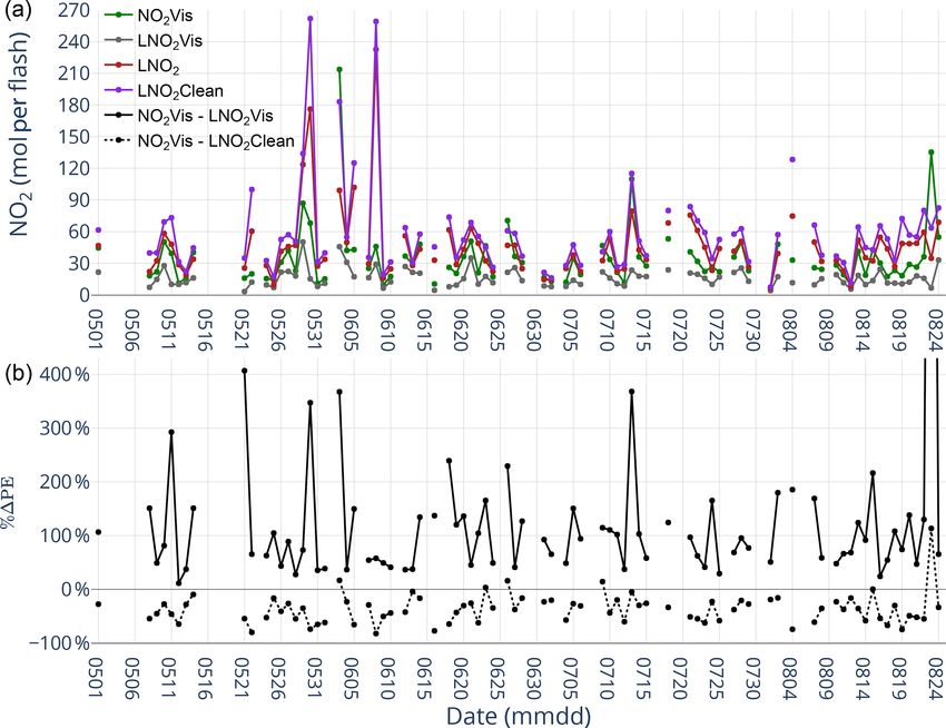
X. Zhang et al.: Estimates of lightning NOx production                                                                      1713

Figure 2. Comparison between total flash densities from ENTLN and WRF-Chem during MJJA 2014.

the TOMRAD lookup table (Bucsela et al., 2013) for clear           AMFLNOx Clean and AMFNO2 Vis , respectively:
and cloudy parts, and NO2 (p) is the modeled NO2 vertical                                    R ptp
profile. Details of these standard parameters and calculation                       (1−fr ) psurf wclear (p)LNO2 (p) dp
                                                                                         R ptp
methods are given in Laughner et al. (2018). LNOx (p) is the                        +fr pcloud wcloudy (p)LNO2 (p) dp
                                                                   AMFLNOx Clean =         R ptp                        ,    (3)
LNOx vertical profile calculated by the difference of vertical
                                                                                             psurf LNOx (p) dp
profiles between WRF-Chem simulations with and without                                 R ptp
                                                                                (1−fr ) psurf wclear (p)NO2 (p) dp
lightning.                                                                          R ptp
   Please note that the CP is a reflectance-weighted pres-                       +fr pcloud wcloudy (p)NO2 (p) dp
                                                                   AMFNO2 Vis =               R ptp                ,         (4)
sure retrieved by the collision-induced O2 –O2 absorption                           (1−fg ) psurf NO2 (p) dp
                                                                                           R ptp
band near 477 nm (Acarreta et al., 2004; Sneep et al., 2008;                         +fg pcloud NO2 (p) dp
Stammes et al., 2008). For a deep convective cloud with
lightning, the CP lies below the geometrical cloud top, which      where fg is the geometric cloud fraction and LNO2 (p) is the
is much closer to that detected by thermal infrared sensors,       modeled LNO2 vertical profile. Besides these AMFs, another
such as CloudSat and the Aqua Moderate Resolution Imag-            AMF called AMFLNO2 Vis is developed for later comparison.
ing Spectrometer (MODIS) (Vasilkov et al., 2008; Joiner                                     R ptp
                                                                                     (1−fr ) psurf wclear (p)NO2 (p) dp
et al., 2012). Hence, much of the tropospheric NO2 measured                              R ptp
                                                                                     +fr pcloud wcloudy (p)NO2 (p) dp
by OMI lies inside the cloud rather than above the cloud top.      AMFLNO2 Vis =                 R ptp                       (5)
In the following, “above cloud” or “below cloud” is relative                            (1−fg ) psurf LNO2 (p) dp
                                                                                               R ptp
to the cloud pressure detected by OMI. The sensitivity study                             +fg pcloud LNO2 (p) dp
of Beirle et al. (2009) compared the chemical composition
from the cloud bottom to that of the cloud top and revealed        A full definition list of the used AMFs is shown in Ap-
that a significant fraction of the NO2 within the cloud orig-      pendix A.
inating from lightning can be detected by the satellite. This
                                                                   2.5   Procedures for deriving LNOx
valuable cloud pressure concept has been applied not only
in the LNOx research but also in the cloud slicing method          VLNOx is re-gridded to 0.05◦ ×0.05◦ grids using the constant
of deriving the UT O3 and NOx (Ziemke et al., 2009, 2017;          value method (Kuhlmann et al., 2014). Then, it is analyzed in
Choi et al., 2014; Strode et al., 2017; Marais et al., 2018). As   1◦ × 1◦ grid boxes with a minimum of 50 valid 0.05◦ × 0.05◦
discussed in Pickering et al. (2016), the ratio of VLNO2 seen      grids to minimize the noise. The main procedures of deriving
by OMI to VLNOx is partly influenced by pcloud . The effects       LNOx are as follows.
of LNO2 below the cloud will be discussed in Sect. 3.4.               CRFs (CRF ≥ 70 %, CRF ≥ 90 %, and CRF = 100 %) and
   To compare our results with those of Pickering et al.           CP ≤ 650 hPa are various criteria of deep convective clouds
(2016) and Lapierre et al. (2020), we calculate their              for OMI pixels (Ziemke et al., 2009; Choi et al., 2014; Pick-
                                                                   ering et al., 2016). The effect of different CRFs on the re-
                                                                   trieved LNOx is explored in Sect. 3.2. Furthermore, another
                                                                   criterion of cloud fraction (CF) is applied to the WRF-Chem
                                                                   results for the successful simulation of convection. The CF
                                                                   is defined as the maximum cloud fraction calculated by the
                                                                   Xu–Randall method between 350 and 400 hPa (Xu and Ran-
                                                                   dall, 1996; Strode et al., 2017). This atmospheric layer (be-
                                                                   tween 350 and 400 hPa) avoids any biases in the simulation
                                                                   of high clouds. We choose CF ≥ 40 % suggested by Strode

www.atmos-meas-tech.net/13/1709/2020/                                                 Atmos. Meas. Tech., 13, 1709–1734, 2020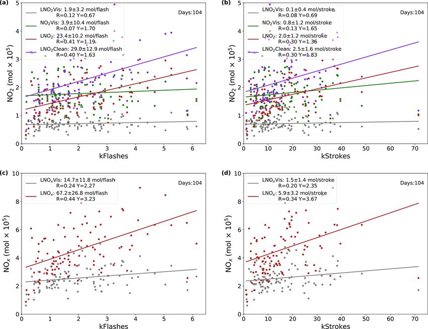
1714                                                                   X. Zhang et al.: Estimates of lightning NOx production

et al. (2017) to determine cloudy or clear for each simulation     3     Results
grid.
   Besides cloud properties, a time period and sufficient          3.1    Criteria determination
flashes (or strokes) are required for fresh LNOx to be de-
tected by OMI. The time window (twindow ) is the hours prior       To determine the suitable criteria from the conditions de-
to the OMI overpass time. twindow is limited to 2.4 h by the       fined in Sect. 2.5, six different combinations are defined (Ta-
mean wind speed at pressure levels 500–100 hPa during OMI          ble 1) and applied to the original data with a linear regression
overpass time and the square root of the 1◦ × 1◦ box over          method (Table 2).
the CONUS (Lapierre et al., 2020). Meanwhile, 2400 flashes            A daily search of the NO2 product for coincident ENTLN
per box and 8160 strokes per box per 2.4 h time window             flash (stroke) data results in 99 (102) valid days under the
are chosen as sufficient for detecting LNOx (Lapierre et al.,      CRF90_ENTLN condition. Taking the flash-type ENTLN
2020). These criteria will result in a low bias in the PE re-      data as an example, the number of valid days decreases from
sults, as Bucsela et al. (2019) found that the PE is larger at     99 to 81 under the CRF90_ENTLN_TL1000_ratio50 con-
small flash rates, which are discarded here. Since our study       dition, while LNOx per flash increases from 52.1 ± 51.1 to
focuses on developing a new AMF and compares results               54.5 ± 48.1 mol per flash. The result is almost the same as
with other works using similar lightning thresholds (Lapierre      that under the CRF90_ENTLN_TL1000 condition, which is
et al., 2020; Pickering et al., 2016), we will only discuss re-    without the condition of more than half of the above-cloud
sults based on the strict criteria in the main text. For compar-   NOx having an LNOx source. Although this indicates the
isons between the criterion of 2400 flashes per box and that       criterion of TL works well, it is better to include the ra-
of one flash per box, scatter diagrams using different light-      tio criterion in case there are some exceptions in the differ-
ning criteria are presented in Appendix B.                         ent AMF methods. Since CF ≥ 40 % leads to a sharp loss
   To ensure that lightning flashes are simulated successfully     of valid numbers and production, it is not a suitable crite-
by WRF-Chem, the threshold of simulated total lightning            rion. Instead the CRF criteria are used. Finally, coincident
flashes (TL) per box is set to 1000, which is fewer than that      ENTLN data, TL ≥ 1000, and ratio ≥ 50 % are chosen as
used by the ENTLN lightning observation, considering the           the thresholds to explore the effects of three different CRF
uncertainty of lightning parameterization. In view of other        conditions (CRF ≥ 70 %, CRF ≥ 90 %, and CRF = 100 %)
NO2 sources in addition to LNO2 , the ratio of modeled light-      on LNOx production (Table 3). Apart from the fewer valid
ning NO2 above cloud (LNO2 Vis) to modeled NO2 above               days under higher CRF conditions (CRF ≥ 90 % and CRF =
cloud (NO2 Vis) is defined to check whether enough LNO2            100 %), LNOx per flash increases from 35.7 ± 36.8 to 54.5
can be detected by OMI. The ratio ≥ 50 % indicates that            ± 48.1 mol per flash and decreases again to 20.8 ± 37.4 mol
more than half of the NOx above the cloud must have an             per flash while LNOx per stroke enhances from 4.1 ± 3.9 to
LNOx source.                                                       7.0 ± 4.8 mol per stroke and drops again to 2.6 ± 4.0 mol per
   Finally, the NO2 lifetime due to oxidation should be taken      stroke (Table 3), as the CRF criterion increases from 70 % to
into account. As estimated by Nault et al. (2017), the lifetime    90 % and to 100 %. When the CRF increases from 90 % to
(τ ) of NO2 in the near field of convections is ∼ 3 h. The         100 %, the LNOx PE decreases because of the higher light-
initial value of NO2 is solved by Eq. (6) as                       ning density with less LNOx (not shown). The increment of
                                                                   LNOx PE caused by the CRF increase from 70 % to 90 % is
NO2 (0) = NO2 (OMI) × e0.5t/τ ,                             (6)
                                                                   opposite to the result of Pickering et al. (2016). This is an
where NO2 (0) is the moles of NO2 emitted at time t = 0,           effect of the consideration of NO2 contamination transported
NO2 (OMI) is the moles of NO2 measured at the OMI over-            from the boundary layer in our method. Although enhanced
pass time, and 0.5t is the half cross grid time, which is 1.2 h,   NOx is often observed in regions with CRF > 70 % (Picker-
assuming that lightning occurred at the center of each 1◦ ×1◦      ing et al., 2016), the following analysis will be based on the
box. For each grid box, the mean LNOx vertical column              criterion of CRF ≥ 90 % considering the contamination by
is obtained by averaging VLNOx values from all regridded           low and midlevel NO2 and comparisons with the results of
0.05◦ ×0.05◦ pixels in the box. This mean value is converted       Pickering et al. (2016) and Lapierre et al. (2020).
to moles of LNOx using the dimensions of the grid box. Two
methods are applied to estimate the seasonal mean LNO2             3.2    Comparison of LNOx production based on
per flash, LNOx per flash, LNO2 per stroke, and LNOx per                  different AMFs
stroke:
                                                                   Lapierre et al. (2020) derived LNO2 production based on the
 1. summation method, dividing the sum of LNOx by the
                                                                   BEHR NO2 product. In order for our results to be compara-
    sum of flashes (or strokes) in each 1◦ × 1◦ box in MJJA
                                                                   ble with those of Pickering et al. (2016) and Lapierre et al.
    2014;
                                                                   (2020), we choose NO2 instead of NOx to derive production
 2. linear regression method, applying the linear regression       per flash (production efficiency, PE). In Fig. 3, time series of
    to daily mean values of LNOx and flashes (or strokes).         NO2 Vis, LNO2 Vis, LNO2 , and LNO2 Clean production per

Atmos. Meas. Tech., 13, 1709–1734, 2020                                              www.atmos-meas-tech.net/13/1709/2020/
X. Zhang et al.: Estimates of lightning NOx production                                                                                                            1715

Table 1. Definitions of the abbreviations for the criteria used in this study.

  Abbreviations                                        Full form (source)
  CRF                                                  Cloud radiance fraction (OMI)
  CP                                                   Cloud optical pressure (OMI)
  CF                                                   Cloud fraction (WRF-Chem)
  TL                                                   Total lightning flashes (WRF-Chem)
  Ratio                                                Modeled LNO2 Vis / modeled NO2 Vis (WRF-Chem)
  CRFα_ENTLN                                           CRF ≥ α+ ENTLN flashes (strokes) ≥ 2400 (8160) (ENTLN)
  CRFα_CF40_ENTLN                                      CRF ≥ α+ ENTLN flashes (strokes) ≥ 2400 (8160) + CF ≥ 40 %
  CRFα_ENTLN_TL1000                                    CRF ≥ α+ ENTLN flashes (strokes) ≥ 2400 (8160) + TL ≥ 1000
  CRFα_CF40_ENTLN_TL1000                               CRF ≥ α+ ENTLN flashes (strokes) ≥ 2400 (8160) + CF ≥ 40 %+ TL ≥ 1000
  CRFα_ENTLN_TL1000_ratio50                            CRF ≥ α+ ENTLN flashes (strokes) ≥ 2400 (8160) + TL ≥ 1000+ ratio ≥ 50 %
  CRFα_CF40_ENTLN_TL1000_ratio50                       CRF ≥ α+ ENTLN flashes (strokes) ≥ 2400 (8160) + CF ≥ 40 % + TL ≥ 1000+ ratio ≥ 50 %
  CRFα_ENTLN1(3.4)_TL1_ratio50                         CRF ≥ α + ENTLN flashes (strokes) ≥ 1 (3.4) + TL ≥ 1+ ratio ≥ 50 %
α has three options: 70 %, 90 %, or 100 %.

Table 2. LNOx production efficiencies for different combinations of criteria defined in Table 1.

                 Condition1                                              ENTLN data          LNOx per flash or           R value        Intercept      Days3
                                                                         type2                LNOx per stroke                          (106 mol)
                 CRF90_ENTLN                                             Flash                        52.1 ± 51.1            0.20           0.21            99
                 CRF90_CF40_ENTLN                                        Flash                        84.2 ± 31.5            0.54          −0.04            70
                 CRF90_ENTLN_TL1000                                      Flash                        61.9 ± 49.1            0.27           0.33            83
                 CRF90_CF40_ENTLN_TL1000                                 Flash                        63.4 ± 52.9            0.38           0.26            38
                 CRF90_ENTLN_TL1000_ratio50                              Flash                        54.5 ± 48.1            0.25           0.39            81
                 CRF90_CF40_ENTLN_TL1000_ratio50                         Flash                        90.0 ± 65.0            0.46           0.15            32
                 CRF90_ENTLN                                             Stroke                         6.7 ± 4.1            0.31           0.23           102
                 CRF90_CF40_ENTLN                                        Stroke                        10.3 ± 3.6            0.55           0.08            79
                 CRF90_ENTLN_TL1000                                      Stroke                         7.5 ± 5.1            0.29           0.38            94
                 CRF90_CF40_ENTLN_TL1000                                 Stroke                         8.6 ± 6.2            0.39           0.27            46
                 CRF90_ENTLN_TL1000_ratio50                              Stroke                         7.0 ± 4.8            0.29           0.42            93
                 CRF90_CF40_ENTLN_TL1000_ratio50                         Stroke                         8.9 ± 7.0            0.39           0.31            40
               1 These conditions are defined in Table 1. 2 The thresholds of ENTLN data are 2400 flashes per box and 8160 strokes per box during the period of
               2.4 h before OMI overpass time. 3 The number of valid days with specific criteria in MJJA 2014.

day over CONUS are plotted for MJJA 2014 with the crite-                                   LNO2 Clean are more sensitive to background NO2 . The ex-
rion of CRF ≥ 90 % and a flash threshold of 2400 flashes per                               tent of the overestimation of NO2 Vis is larger than that of
2.4 h. LNO2 PEs are mostly in the range from 20 to 80 mol                                  LNO2 Clean in highly polluted regions, while it is usually op-
per flash. LNO2 Vis PEs are smaller than LNO2 PEs, which                                   posite in most regions.
contain LNO2 below clouds. The simulation of GMI in Pick-                                     Figure 4 shows the linear regression for ENTLN data ver-
ering et al. (2016) indicated that 25 %–30 % of the LNOx                                   sus NO2 Vis, LNO2 Vis, LNO2 , and LNO2 Clean with the
column lies below the CP, while the ratio in our WRF-Chem                                  same criteria as shown in Fig. 3. LNO2 Clean PE (the largest
simulation is 56 ± 20 %. The effect of cloud properties on                                 slope) is 25.2 ± 22.3 mol NO2 per flash with a correlation
LNOx PE will be discussed in more detail in Sect. 3.4. Gener-                              of 0.25 and 2.3 ± 2.1 mol NO2 per stroke with a correla-
ally, the order of estimated daily PEs is LNO2 Clean > LNO2                                tion of 0.22. As shown in Fig. 3, positive percent differ-
> NO2 Vis > LNO2 Vis. The percent difference in the esti-                                  ences between NO2 Vis PE and LNO2 Clean PE occur much
mated PE (1PE) between NO2 Vis and LNO2 Vis indicates                                      less often than negative differences. As a result, NO2 Vis PE
a certain amount of background NO2 exists above clouds.                                    (17.1 ± 17.2 mol NO2 per flash and 0.4 ± 1.0 mol NO2 per
Overall, the tendency of that 1PE is consistent with another                               stroke) is smaller than LNO2 Clean PE using the linear re-
1PE between NO2 Vis and LNO2 Clean. When the region                                        gression method.
is highly polluted (1PE between NO2 Vis and LNO2 Vis is                                       In order to compare our result with that of Lapierre et al.
larger than 200 %), PEs based on NO2 Vis and LNO2 Clean                                    (2020), we tried to remove the CP ≤ 650 hPa, TL ≥ 1000,
are significantly overestimated. In other words, NO2 Vis and                               and ratio ≥ 50 % conditions from criteria. But, our result

www.atmos-meas-tech.net/13/1709/2020/                                                                               Atmos. Meas. Tech., 13, 1709–1734, 2020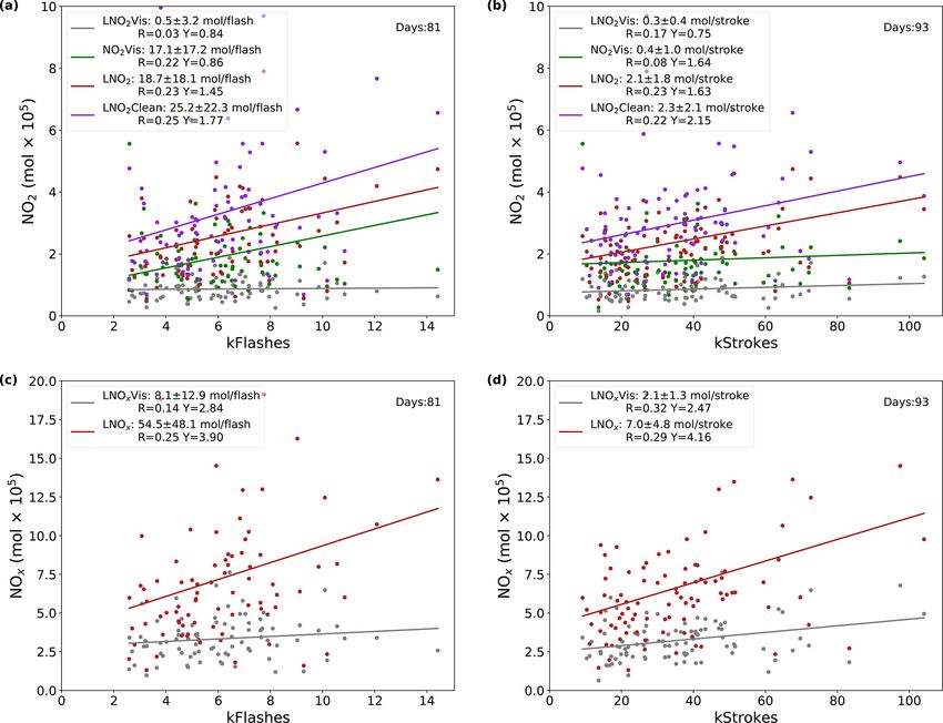
1716                                                                                      X. Zhang et al.: Estimates of lightning NOx production

Table 3. LNOx production efficiencies for different thresholds of CRF with coincident ENTLN data, TL ≥ 1000, and ratio ≥ 50 %.

             CRF (%)        ENTLN data type1            LNOx per flash or LNOx per stroke                R value       Intercept (105 mol)         Days2
             70             Flash                                                     35.7 ± 36.8            0.21                        4.91          85
             90             Flash                                                     54.5 ± 48.1            0.25                        3.90          81
             100            Flash                                                     20.8 ± 37.4            0.13                        5.67          71
             70             Stroke                                                      4.1 ± 3.9            0.21                        5.16          96
             90             Stroke                                                      7.0 ± 4.8            0.29                        4.16          93
             100            Stroke                                                      2.6 ± 4.0            0.14                        5.41          82
           1 The thresholds of ENTLN data are 2400 flashes per box and 8160 strokes per box during the period of 2.4 h before OMI overpass time. 2 The number
           of valid days with specific criteria in MJJA 2014.

Figure 3. (a) Time series of NO2 Vis, LNO2 Vis, LNO2 , and LNO2 Clean production per day over the CONUS for MJJA 2014 with CRF ≥
90 % and a flash threshold of 2400 flashes per 2.4 h. (b) Time series of the percent differences between NO2 Vis and LNO2 Vis and the percent
differences between NO2 Vis and LNO2 Clean with CRF ≥ 90 %. The value of the black dot on 23 August (not shown) is 1958 %.

based on daily summed NO2 Vis values (3.8 ± 0.5 mol per                                   3. The surface pressure is now calculated according to
stroke) is still larger than the value of 1.6± 0.1 mol per stroke                            Zhou et al. (2009).
mentioned in Lapierre et al. (2020). This may be caused by
the different version of the BEHR algorithm, as Lapierre                               The detailed log of changes is available at https:
et al. (2020) used BEHR v3.0A and our algorithm is based                               //github.com/CohenBerkeleyLab/BEHR-core/blob/master/
on BEHR v3.0B (Laughner et al., 2019). The input of SNO2                               Documentation/Changelog.txt (last access: 20 March 2020).
in both versions is from the NASA standard product v3, and                             Note that Lapierre et al. (2020) used the monthly NO2
the major improvements of BEHR v3.0B are listed below.                                 profile. While the daily profile is used in our study and the
                                                                                       interval of our outputs from WRF-Chem is 30 min, which is
  1. The profile (v3.0B) closest to the OMI overpass time                              more frequent than 1 h in the BEHR daily product, the AMF
     was selected instead of the last profile (v3.0A) before                           could be affected by different NO2 profiles. In view of these
     the OMI overpass.                                                                 factors, we compare different methods based on our data to
                                                                                       minimize these effects.
  2. The AMF uses a variable tropopause height as opposed                                 Meanwhile, LNO2 PE (18.7±18.1 mol per flash and 2.1±
     to the fixed 200 hPa tropopause.                                                  1.8 mol per stroke) is between LNO2 Clean PE and NO2 Vis

Atmos. Meas. Tech., 13, 1709–1734, 2020                                                                        www.atmos-meas-tech.net/13/1709/2020/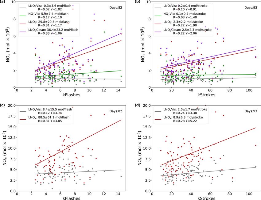
X. Zhang et al.: Estimates of lightning NOx production 1717
PE, which coincides with the daily results in Fig. 3. Further- higher than UT background NO2 concentrations. However,
more, the LNOx PE based on the linear regression of daily the ratio profile in Fig. 7e has one peak between the cloud
summed values, the same method used in Pickering et al. pressure and tropopause as background NO2 increases and
(2016), is 114.8 ± 18.2 mol per flash (or 17.8 ± 2.9 mol per LNO2 decreases. Besides, the percentage of UT background
stroke), which is larger than 91 mol per flash in Pickering NO2 in polluted regions is steady and higher than that in
et al. (2016), possibly due to the differences in geographic clean regions.
location, lightning data, and chemistry model. Table 4 presents the relative changes among
The mean and standard deviation of LNO2 PE under three methods in six cities. The difference be-
CRF ≥ 90 % using the summation method is 46.2 ± 35.1 mol tween AMFLNO2 (Eq. R7) and AMFLNO2 Clean (Eq. 9)
ptp
per flash and 9.9 ± 8.1 mol per stroke, while LNOx PE is is the numerator: pcloud wcloudy (p)NO2 (p) dp and
R ptp
125.6 ± 95.9 mol per flash and 26.7 ± 21.6 mol per stroke w (p)LNO (p) dp. When the ratio of LNO
pcloud cloudy 2 2
(Fig. 5). The LNO2 PE and LNOx PE are both higher in the is higher or the region is cleaner, the relative difference is
southeast US (denoted by the red box in Fig. 5, 25–37◦ N, smaller (e.g. 5.0 %–12.0 %, Fig. 7d–f). The largest relative
75–95◦ W), consistent with Lapierre et al. (2020) and Buc- difference (46.3 %) occurs when the ratio of background
sela et al. (2019). Compared with Fig. 3, Fig. 6a and b present NO2 is continuously high in the UT (Fig. 7c). As a result,
some large differences between NO2 Vis PE and LNO2 Vis our approach is less sensitive to background NO2 and
PE, which are consistent with what we expect for polluted more suitable for convective cases over polluted locations.
regions. Meanwhile, the differences between LNO2 PE and In contrast, production estimated by our method is larger
NO2 Vis PE depend on background NO2 , the strength of up- than that based on NO2 Vis due to the LNO2 below the
draft, and the profile. The negative differences are caused by cloud. When the cloud is higher, in particular the peak
background NO2 carried by the updraft while parts of the of the LNO profile is lower than the cloud (Fig. 7b).
below-cloud LNO2 result in LNO2 PE higher than NO2 Vis The relative difference is larger (121.2 %) because more
PE (Fig. 6c). Figure 6d shows that the ratio of LNO2 Vis to LNO2 can not be included in the NO2 Vis, which has
LNO2 ranges from 10 % to 80 %. This may be caused by the been discussed in Sect. 3.2. The relative change between
height of the clouds and the profile of LNO2 . If the CP is AMF
R ptp LNO2 Clean (Eq. 9) and AMF R pNO 2 Vis (Eq. 8) depends on
near 300 hPa, the ratio should be smaller because of the cov- dp/ tp
w
pcloud cloudy (p)LNO 2 (p) psurf cloudy (p)LNO2 (p) dp,
w
erage of clouds. While peaks of the LNO2 profile are below which is also affected by cloud, not the background NO2 .
the CP, the ratio would also be smaller. Therefore, a better The largest relative change (153.8 %) occurs at New Orleans,
understanding of the LNO2 profile and LNOx below clouds which has the lowest cloud pressure and consequently the
is required. smallest visible column.
3.3 Effects of tropospheric background on LNOx 3.4 Effects of cloud and LNOx parameterization on
production LNOx production
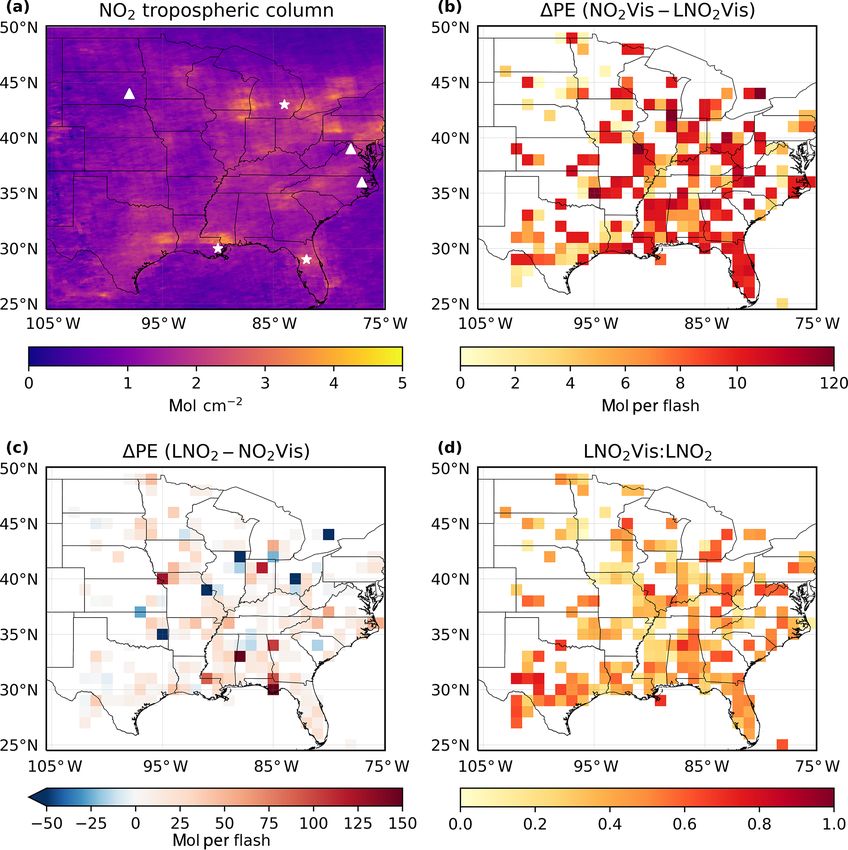
With respect to the LNO2 production, the patterns in Fig. 6 Figure 8a presents the daily distribution of CP and the ra-
indicate the improvement of our approach is different in pol- tio of LNO2 Vis to LNO2 during MJJA 2014 with the cri-
luted and clean regions. To simplify the quantification, we teria defined in Sect. 3.1 under CRF ≥ 90 %. Since the ra-
select six grids with similar NO2 profiles (∼ 100 pptv) above tio of LNO2 Vis to LNO2 decreases from 0.8 to 0.2 as the
the cloud with CRF = 100 %. These grid boxes contain the cloud pressure decreases from 600 to 300 hPa, NO2 Vis PE is
polluted and clean cities denoted by stars and triangles in smaller than LNO2 PE in relatively clean areas as shown in
Fig. 6a, respectively. Then, the differences between AMFs Fig. 4. Apart from LNO2 Vis, the LNO2 PE is also affected by
are dependent on fewer parameters. CP. For LNO2 PEs larger than 30 mol per stroke, the CPs are
R ptp
wcloudy (p)NO2 (p) dp all smaller than 550 hPa (Fig. 8b). However, smaller LNO2
p
AMFLNO2 = cloudR ptp (7) PEs (< 30 mol per stroke) occur on all levels between 650
psurf LNO2 (p) dp and 200 hPa. Because of the limited number of large LNO2
R ptp
p wcloudy (p)NO2 (p) dp PEs and lightning data, we cannot derive the relationship be-
AMFNO2 Vis = cloud R ptp (8) tween LNO2 PE and cloud pressure or other lightning prop-
pcld NO2 (p) dp erties at this stage. Because the CP only represents the devel-
R ptp
p wcloudy (p)LNO2 (p) dp opment of clouds, the vertical structure of flashes can not be
AMFLNO2 Clean = cloud R ptp (9) derived from the CP values only. As discussed in several pre-
psurf LNO2 (p) dp
vious studies, the flash channel length varies and depends on
Figure 7 compares the mean profiles of NO2 , background the environmental conditions (Carey et al., 2016; Mecikalski
NO2 and background NO2 ratio in polluted and clean grids. and Carey, 2017; Fuchs and Rutledge, 2018). Davis et al.
Generally, the profiles of the ratio of background NO2 to to- (2019) compared two kinds of flash: normal flashes and
tal NO2 are C shaped because UT LNO2 concentrations are anomalous flashes. Because updrafts are stronger and flash
www.atmos-meas-tech.net/13/1709/2020/ Atmos. Meas. Tech., 13, 1709–1734, 2020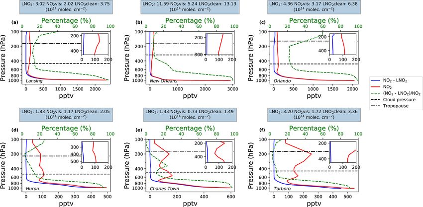
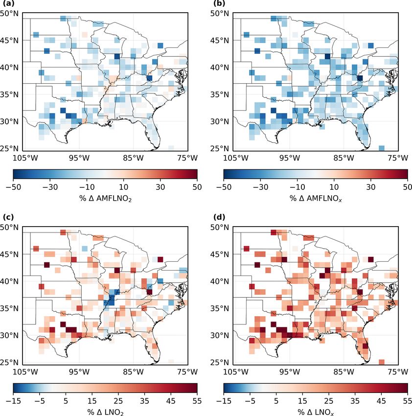
1718                                                                   X. Zhang et al.: Estimates of lightning NOx production

Figure 4. (a) Daily NO2 Vis, LNO2 Vis, LNO2 , and LNO2 Clean versus ENTLN total flash data. (b) Same as (a) but for strokes. (c) Daily
LNOx Vis and LNOx versus total flashes. (d) Same as (c) but for strokes.

rates are higher in anomalous storms, UT LNOx concentra-             pact of LNOx parameterization on LNOx estimation, we
tions are larger in anomalous than normal polarity storms. In        apply another WRF-Chem NO2 profile setting (2× base
general, normal flashes are coupled with an upper-level pos-         flash rate, 500 mol NO per flash, hereinafter referred to as
itive charge region and a midlevel negative charge region,           “2 × 500 mol NO per flash”) to a priori profiles and evaluate
while anomalous flashes are opposite (Williams, 1989). It is         the changes in AMFLNO2 , AMFLNOx , LNO2 PE, and LNOx
not straightforward to estimate the error resulting from the         PE. For the linear regression method (Fig. 9), LNO2 PE is
vertical distribution of LNOx . There are mainly two methods         29.8 ± 20.5 mol per flash, which is 59.4 % larger than the ba-
of distributing LNOx in models: LNOx profiles (postconvec-           sic one (18.7 ± 18.1 mol per flash). Meanwhile, LNOx PE
tion) in which LNOx has already been redistributed by con-           (increasing from 54.5±48.1 mol per flash to 88.5±61.1 mol
vective transport and LNOx production profiles (preconvec-           per flash) also depends on the configuration of LNO produc-
tion) made before the redistribution of convective transport         tion in WRF-Chem. The comparison between Figs. 4 and 9
(Allen et al., 2012; Luo et al., 2017). However, given the sim-      shows that LNO2 Clean PE and LNO2 PE are more similar
ilarity of results compared to other LNOx studies, we believe        while LNO2 PE and NO2 Vis PE present the same tendency.
that our 1◦ × 1◦ results based on postconvective LNOx pro-           It remains unclear as to whether the NO–NO2 –O3 cycle or
files are sufficient for estimating average LNOx production.         other LNOx reservoirs account for the increment of LNOx
   The LNO production settings in WRF-Chem varied in                 PE. This would need detailed source analysis in WRF-Chem
different studies. Zhao et al. (2009) set a NOx produc-              and is beyond the scope of this study.
tion rate of 250 mol NO per flash in a regional-scale model,            Figure 10 shows the average percentage changes in
while Bela et al. (2016) chose 330 mol NO per flash used             AMFLNO2 , AMFLNOx , LNO2 , and LNOx between retrievals
by Barth et al. (2012). Wang et al. (2015) assumed ap-               using profiles based on 1×200 and 2×500 mol NO per flash.
proximately 500 mol NO per flash, which was derived by               These results were obtained by averaging data over MJJA
a cloud-scale chemical transport model and in-cloud air-             2014 based on the method described in Sect. 2.5 with the
craft observations (Ott et al., 2010). To illustrate the im-         criterion of CRF ≥ 90 %. The effects on LNO2 and LNOx

Atmos. Meas. Tech., 13, 1709–1734, 2020                                                 www.atmos-meas-tech.net/13/1709/2020/
X. Zhang et al.: Estimates of lightning NOx production                                                                                 1719

Figure 5. (a, c) Maps of 1◦ ×1◦ gridded values of mean LNOx and LNO2 production per flash with CRF ≥ 90 % for MJJA 2014. (b, d) Same
as (a) and (c) except for strokes. The southeastern US is denoted by the red box in panels (a)–(d).

Table 4. The percent changes in the estimated production when using different methods based on the same a priori profiles.

                       City∗                (LNO2 Clean – LNO2 )/LNO2   (LNO2 – TropVis)/TropVis   (LNO2 Clean-TropVis)/TropVis
                       Lansing                                 24.2 %                    49.5 %                               85.6 %
        Polluted       New Orleans                             13.3 %                   121.2 %                              153.8 %
                       Orlando                                 46.3 %                    37.5 %                              101.3 %
                       Huron                                   12.0 %                    56.4 %                               75.2 %
        Clean          Charles Town                            12.0 %                    82.2 %                              104.1 %
                       Tarboro                                  5.0 %                    86.0 %                               95.3 %
      ∗ Locations are denoted in Fig. 6a.

retrieval from increasing LNO profile values show mostly                  above the clouds. The magnitude of an increasing denom-
the same tendency: smaller AMFLNO2 and AMFLNOx lead                       inator could be different than that of an increasing numer-
to larger LNO2 and LNOx , but the changes are regionally                  ator, resulting in a different effect on the AMFLNO2 and
dependent. This is caused by the nonlinear calculation of                 AMFLNOx . As mentioned in Zhu et al. (2019), the lightning
AMFLNO2 and AMFLNOx . As the contribution of LNO2 in-                     densities in the southeast US might be overestimated using
creases, both the numerator and denominator of Eq. (2) in-                the 2 × 500 mol NO per flash setting and the same lightning
crease. Note that the LNO2 accounts for a fraction of NO2                 parameterization as ours. Fortunately, the AMFs and esti-

www.atmos-meas-tech.net/13/1709/2020/                                                      Atmos. Meas. Tech., 13, 1709–1734, 2020
1720 X. Zhang et al.: Estimates of lightning NOx production Figure 6. (a) Mean (MJJA 2014) NO2 tropospheric column. Polluted cities are denoted by stars (Lansing, New Orleans, and Orlando) while clean cities are denoted by triangles (Huron, Charles Town, and Tarboro). (b) The differences of the estimated mean production efficiency between NO2 Vis and LNO2 Vis with CRF ≥ 90 %. (c) The same differences as (b) but between LNO2 and NO2 Vis. (d)The ratio of LNO2 Vis to LNO2 . mated LNO2 change little in that region. Because the south- ysis is false in some regions, it allows the calculation of east US has the highest flash density (Fig. 2), the NO2 in the an upper limit on the NO2 due to LNO and LNO2 profiles. numerator of AMF is dominated by LNO2 . Both the SCD As discussed in Laughner and Cohen (2017), the scattering and VCD will increase when the model uses higher LNO2 . weights are uniform under cloudy conditions and the sensi- In other words, the sensitivity to the LNO setting decreases tivity of NO2 is nearly constant with different pressure levels and the relative distribution of LNO2 matters. because of the high albedo. However, the relative distribution Figure 11 shows the comparison of the mean LNO of LNO2 within the UT should be taken carefully into con- and LNO2 profiles in two specific regions where the 2 × sideration. If the LNO2 /NO2 above the cloud is large enough 500 mol NO per flash setting leads to lower and higher LNO2 (Fig. 11a), the AMFLNO2 is largely determined by the ratio PEs, respectively. The first one (Fig. 11a) is the region (36– of LNO2 Vis to LNO2 , which is related to the relative distri- 37◦ N, 89–90◦ W) containing the minimal negative percent bution. When the condition of high LNO2 /NO2 is not met, change in LNO2 (Fig. 10c). The second one (31–32◦ N, 97– both relative distribution and ratio are important (Fig. 11b). 98◦ W), Fig. 11b, has the largest positive percent change To clarify this, we applied the same sensitivity test of in LNO2 (Fig. 10c). Although the relative distributions of different simulating LNO amounts for all four methods mean LNO and LNO2 profiles are similar in both regions, mentioned in Sect. 2.4: LNO2 , LNO2 Vis, LNO2 Clean, and the magnitude differs by a factor of 10. This phenomenon NO2 Vis (Fig. 12). Note that the threshold for CRF is set implies that the performance of lightning parameterization in to 100 % to simplify Eq. (2) to Eq. (7). The overall differ- WRF-Chem is regionally dependent, and an unrealistic pro- ences of LNO2 Clean and NO2 Vis are smaller than those of file could appear in the UT. Although this sensitivity anal- LNO2 and LNO2 Vis. Comparing the numerator and denom- Atmos. Meas. Tech., 13, 1709–1734, 2020 www.atmos-meas-tech.net/13/1709/2020/
X. Zhang et al.: Estimates of lightning NOx production                                                                               1721

Figure 7. Comparisons of mean WRF-Chem NO2 and background NO2 profiles in six grids with CRF ≥ 100 % on specific days during
MJJA 2014. The (a), (b), and (c) data are selected from polluted regions (stars in Fig. 6a) while the (d), (e), and (f) data are from clean
regions (triangles in Fig. 6a). The green dashed lines are the mean ratio profiles of background NO2 to total NO2 . The zoomed figures show
the profiles from the cloud pressure to the tropopause. The titles present the mean productions based on three different methods mentioned
in Sect. 2.4.

Figure 8. Kernel density estimation of the (a) daily ratio of LNO2 Vis to LNO2 and (b) daily LNO2 production efficiency versus the daily
cloud pressure measured by OMI with CRF ≥ 90 % for MJJA 2014. The kernel density estimation was generated by kdeplot in the Python
package named seaborn.

inator in the equations, it is clear why the impact of different        LNO2 vertical column, respectively. As a result, the negative
simulating LNO amounts is smaller in Fig. 12c and d. For                values in Fig. 12a are caused by the part of LNO2 below the
LNO2 Clean and NO2 Vis, both the SCD and VCD will in-                   cloud. The uncertainty of retrieved LNO2 and LNOx PEs is
crease (decrease) when more (less) LNO2 or NO2 presents.                driven by this error, and we conservatively estimate this to be
The difference between Fig. 12a and b is the denomina-                  ±13 % and ±25 %, respectively.
tor: the total tropospheric LNO2 vertical column and visible

www.atmos-meas-tech.net/13/1709/2020/                                                      Atmos. Meas. Tech., 13, 1709–1734, 2020
1722                                                                      X. Zhang et al.: Estimates of lightning NOx production

Figure 9. Same as Fig. 4 except for the 2 × 500 mol NO per flash configuration.

4   Uncertainty analysis                                                pressures to the GLOBE surface pressures and arrived at the
                                                                        largest bias of 1.5 %. Based on the largest bias, we vary the
The uncertainties of the LNO2 and LNOx PEs are esti-                    surface pressure (limited to less than 1020 hPa), and the un-
mated following Pickering et al. (2016), Allen et al. (2019),           certainty can be neglected.
Bucsela et al. (2019), Laughner et al. (2019) and Lapierre                 The error in cloud radiance fraction is transformed from
et al. (2020). We determine the uncertainty due to BEHR                 cloud fraction using
tropopause pressure, cloud radiance fraction, cloud pressure,
surface pressure, surface reflectivity, profile shape, profile lo-                   ∂fr
                                                                        σ = 0.05 ·                  ,                             (10)
cation, Vstrat , the detection efficiency of lightning, twindow ,                    ∂fg   fg,pix
and LNO2 lifetime numerically by perturbing each parame-
ter in turn and re-retrieving the LNO2 and LNOx with the                where fr is the cloud radiance fraction, fg is the cloud frac-
perturbed values (Table 5).                                             tion, and fg,pix is the cloud fraction of a specific pixel. We
   The GEOS-5 monthly tropopause pressure, which is con-                calculate ∂fr /∂fg under fg,pix by the relationship between
sistent with the NASA standard product, is applied instead              all binned fr and fg with the increment of 0.05 for the each
of the variable WRF tropopause height to evaluate the un-               specific OMI orbit. Considering the relationship, the error in
certainty (6 % for LNO2 PE and 4 % for LNOx PE) caused                  cloud fraction is converted to an error in cloud radiance frac-
by the BEHR tropopause pressure. The cloud pressure bias                tion of 2 % for the LNO2 and LNOx PEs.
is given as a function of cloud pressure and fraction by Acar-             The accuracy of the 500 m MODIS albedo product is usu-
reta et al. (2004), implying an uncertainty of 32 %, the most           ally within 5 % of albedo observations at the validation sites,
likely uncertainty in the production analysis, for LNO2 PE              and those exceptions with low-quality flags have been found
and 34 % for LNOx PE. The resolution of GLOBE terrain                   to be primarily within 10 % of the field data (Schaaf et al.,
height data is much higher than the OMI pixel, and a fixed              2011). Since we use the bidirectional reflectance distribution
scale height is assumed in the BEHR algorithm. As a result,             function (BRDF) data directly, rather than including a radia-
Laughner et al. (2019) compared the average WRF surface                 tive transfer model, 14 % Lambertian equivalent reflectivity

Atmos. Meas. Tech., 13, 1709–1734, 2020                                                     www.atmos-meas-tech.net/13/1709/2020/
X. Zhang et al.: Estimates of lightning NOx production 1723
Figure 10. Average percent differences in (a) AMFLNO2 , (b) AMFLNOx , (c) LNO2 , and (d) LNOx with CRF ≥ 90 % over MJJA 2014.
Differences between profiles are generated by 2 × 500 and 1 × 200 mol NO per flash.
Table 5. Uncertainties for the estimation of LNO2 per flash, LNOx per flash, LNO2 per stroke, and LNOx per stroke.
Type Perturbation LNO2 LNOx LNO2 LNOx
per flash5 per flash5 per stroke5 per stroke5
BEHR tropopause pressure1 NASA product tropopause 6 4 6 4
Cloud radiance fraction1 ±5 % 2 2 2 2
Cloud pressure2 Variable 32 34 32 34
Surface pressure1 ±1.5 % 0 0 0 0
Surface reflectivity1 ±17 % 0 0 0 0
LNO2 profile1 2 × 500 mol NO per flash 13 25 13 25
Profile location1 Quasi-Monte Carlo 0 1 0 1
Lightning detection efficiency3 IC: ±16 %, CG: ±5 % 15 15 15 15
twindow 3 2–4 h 10 10 8 8
LNOx lifetime3 2–12 h 24 24 24 24
Vstrat 4 – 10 10 10 10
Systematic errors in slant column4 – 5 5 5 5
Tropospheric background4 – 10 10 10 10
NO/NO2 4 20 % ± 15 % 0 15 0 15
Net – 49 56 48 56
PEuncertainty = (Errorrising perturbed value - Errorlowering perturbed value )/2, where Errorperturbed value = (PE perturbed value – PEoriginal value )/PEoriginal value .
1 Laughner et al. (2019). 2 Acarreta et al. (2004). 3 Lapierre et al. (2020). 4 Allen et al. (2019) and Bucsela et al. (2019). 5 Uncertainty (%).
www.atmos-meas-tech.net/13/1709/2020/ Atmos. Meas. Tech., 13, 1709–1734, 20201724 X. Zhang et al.: Estimates of lightning NOx production Figure 11. LNO and LNO2 profiles with different LNO settings in (a) the region containing the minimal negative percent change in LNO2 and (b) the region containing the largest positive percent change in LNO2 when the LNO setting is changed from 1 × 200 to 2 × 500 mol NO per flash, averaged over MJJA 2014. The profiles using 1×200 (2×500) mol NO per flash are shown in blue (red) lines. Solid (dashed) green lines are the mean ratio of LNO2 to NO2 with 1 × 200 (2 × 500) mol NO per flash. (LER) error and 10 % uncertainty are combined to get a per- (Lapierre et al., 2020). It is found that the resulting uncer- turbation of 17 % (Laughner et al., 2019). The uncertainty tainty of detection efficiency is 15 % in the production anal- due to surface reflectivity can be neglected with the 17 % per- ysis. We have used the twindow of 2.4 h for counting ENTLN turbation. flashes and strokes to analyze LNO2 and LNOx production. As discussed at the end of Sect. 3.4, another setting of Because twindow derived from the ERA5 reanalysis can not LNO2 (2 × 500 mol NO per flash) is applied to determine the represent the variable wind speeds, a sensitivity test is per- uncertainty of the lightning parameterization and the verti- formed which yields an uncertainty of 10 % for production cal distribution of LNO in WRF-Chem. Differences between per flash and 8 % for production per stroke using twindow of the two profiles lead to an uncertainty of 13 % and 25 % in 2 and 4 h. Meanwhile, the lifetime of UT NOx ranges from the resulting PEs of LNO2 and LNOx . Another sensitivity 2 to 12 h depending on the convective location, the methyl test allows each pixel to shift by −0.2, 0, or +0.2 ◦ in the peroxy nitrate and alkyl, and multifunctional nitrates (Nault directions of longitude and latitude, taking advantage of the et al., 2017). The lifetime (τ ) of NO2 in Eq. (6) is replaced by high-resolution profile location in WRF-Chem. The resulting 2 and 12 h to determine the uncertainty as 24 % due to life- uncertainty of LNOx PE is 1 %, including the error of trans- time. This is comparable with the uncertainty (25 %) caused port and chemistry by shifting pixels. by lightning parameterization for the LNOx type. Compared to the NASA standard product v2, Krotkov Recent studies revealed that the modeled NO/NO2 ratio et al. (2017) demonstrated that the noise in Vstrat is 1 × departs from the data in the SEAC4 RS aircraft campaign 1014 cm−2 . Errors in polluted regions can be slightly larger (Travis et al., 2016; Silvern et al., 2018). Silvern et al. (2018) than this value, while errors in the cleanest areas are typically attributed this to the positive interference on the NO2 mea- significantly smaller (Bucsela et al., 2013). We estimated the surements or errors in the cold-temperature NO−NO2 −O3 uncertainty of the Vstrat component and the slant column er- photochemical reaction rate. We assign a 20 % bias with rors to be 10 % and 5 %, respectively, following Allen et al. ±15 % uncertainty to this error considering the possible posi- (2019). tive NO2 measurement interferences (Allen et al., 2019; Buc- Based on the standard deviation of the detection efficiency sela et al., 2019) and estimate the uncertainty to be 15 % for estimation over the CONUS relative to LIS, ENTLN de- LNOx PE. tection efficiency uncertainties are ± 16 % for total and IC In addition, the estimation of LNOx PE also depends on flashes and strokes. Due to the high detection efficiency of the tropospheric background NO2 . In our method, the main CG over the CONUS, the uncertainty is estimated to be ±5 % factors affecting this factor are the emissions inventory and Atmos. Meas. Tech., 13, 1709–1734, 2020 www.atmos-meas-tech.net/13/1709/2020/
You can also read