Sensitivity of precipitation and temperature over the Mount Kenya area to physics parameterization options in a high-resolution model simulation ...
←
→
Page content transcription
If your browser does not render page correctly, please read the page content below
Geosci. Model Dev., 14, 2691–2711, 2021
https://doi.org/10.5194/gmd-14-2691-2021
© Author(s) 2021. This work is distributed under
the Creative Commons Attribution 4.0 License.

Sensitivity of precipitation and temperature over the Mount Kenya
area to physics parameterization options in a high-resolution model
simulation performed with WRFV3.8.1
Martina Messmer1,2,3 , Santos J. González-Rojí1,2 , Christoph C. Raible1,2 , and Thomas F. Stocker1,2
1 Climate and Environmental Physics, University of Bern, Bern, Switzerland
2 Oeschger  Centre for Climate Change Research, University of Bern, Bern, Switzerland
3 School of Earth Sciences, The University of Melbourne, Melbourne, Victoria, Australia

Correspondence: Martina Messmer (martina.messmer@climate.unibe.ch)

Received: 15 October 2020 – Discussion started: 12 November 2020
Revised: 10 February 2021 – Accepted: 18 March 2021 – Published: 18 May 2021

Abstract. Several sensitivity experiments with the Weather        the Grell–Freitas cumulus parameterization in the domains
Research and Forecasting (WRF) model version 3.8.1 have           with resolutions > 5 km also provides reasonable results for
been performed to find the optimal parameterization setup         2 m temperature with respect to gridded observational and
for precipitation amounts and patterns around Mount Kenya         weather station data.
at a convection-permitting scale of 1 km. Hereby, the focus
is on the cumulus scheme, with tests of the Kain–Fritsch,
the Grell–Freitas, and no cumulus parameterizations. In ad-
dition, two longwave radiation schemes and two planetary          1   Introduction
boundary layer parameterizations are evaluated, and differ-
ent nesting ratios and numbers of nests are tested. The pre-      East Africa, including Kenya, has anomalously dry cli-
cipitation amounts and patterns are compared against a large      mate conditions compared to many other equatorial regions
amount of weather station data and three gridded observa-         around the globe (e.g. Trewartha, 1981; Nicholson, 2017).
tional data sets. The temporal correlation of monthly pre-        The precipitation patterns in East Africa are very heteroge-
cipitation sums show that fewer nests lead to a more con-         neous, which can be attributed to the variety and complex-
strained simulation, and hence the correlation is higher. The     ity of large-scale controls, i.e. topography, influence from
pattern correlation with weather station data confirms this re-   the ocean, the dynamics of the tropical circulation, and lakes
sult, but when comparing it to the most recent gridded ob-        (Nicholson, 2017). The topography, in particular the Turkana
servational data set the difference between the number of         channel between the Ethiopian and East African highlands
nests and nesting ratios is marginal. The precipitation pat-      in Kenya, exerts a strong steering effect on the low-level
terns further reveal that using the Grell–Freitas cumulus pa-     flow on timescales from seasons to days (Paegle and Geisler,
rameterization in the domains with resolutions > 5 km pro-        1986; Slingo et al., 2005). The Turkana jet has an influence
vides the best results when it comes to precipitation patterns    on the local climate and especially on precipitation, and a
and amounts. If no cumulus parameterization is used in any        study by Nicholson (2016a) suggests that it might even be
of the domains, the temporal correlation between gridded and      responsible for the suppression of the summer rainy season
in situ observations and simulated precipitation is especially    in northwestern Kenya. The zonal circulation over the In-
poor with more nests. Moreover, even if the patterns are cap-     dian Ocean further influences precipitation in Kenya, as it
tured reasonably well, a clear overestimation in the precipi-     is located under subsiding air masses, leading to the afore-
tation amounts is simulated around Mount Kenya when us-           mentioned aridity over an equatorial region (Pohl and Cam-
ing no cumulus scheme in all domains. The experiment with         berlin, 2011; Nicholson, 2017). Weak equatorial zonal circu-
                                                                  lations are typically associated with floods at the coasts of

Published by Copernicus Publications on behalf of the European Geosciences Union.
2692                        M. Messmer et al.: Sensitivity of precipitation to physics parameterizations over Mount Kenya

East Africa, which coincide with scarce rain over Indone-             son rather than a decline in daily precipitation, as the tropical
sia (Hastenrath and Polzin, 2004, 2005). This circulation and         rainband moves faster to the north during the long rains.
thus the intensity and the vertical extent of the subsidence             The rather sparse observation network in East Africa and
account for variations in the inter-annual rainfall variability       thus Kenya, in combination with the aforementioned com-
over Kenya (Pohl and Camberlin, 2011; Nicholson, 2017).               plexity of the climate, conspires against obtaining a better
The second-largest freshwater lake in the world, Lake Vic-            understanding of all the involved processes that dominate the
toria, also contributes to rainfall in this area. It generates its    climate, as well as its changes. To overcome this issue, cli-
own mesoscale atmospheric circulation system that leads to            mate models, and regional climate models in particular, could
high rainfall amounts over the lake, where lake surface tem-          help understanding those processes in more detail. Neverthe-
peratures are strongly related to the rainfall amounts (Sun           less, capturing the convective precipitation in the tropics cor-
et al., 2014). Furthermore, local thunderstorms with heavy            rectly is also a challenge for regional climate models, and
precipitation can be triggered over Lake Victoria, rendering          this is why several studies focus on the evaluation of their
the lake–land breeze but also large-scale moisture availabil-         performance in different regions (e.g. Rauscher et al., 2010;
ity as the main control (Thiery et al., 2015; Woodhams et al.,        Kendon et al., 2017; Brune et al., 2020; Wu et al., 2020).
2019).                                                                   Only in the past few years has the number of climate sim-
   All these large-scale controls lead to the fact that the cli-      ulations increased over Africa generally or over East Africa
mate in Kenya is characterized by two rainy seasons. The              specifically. At the same time, the resolution of these simu-
March–April–May (MAM) season is often termed as “long                 lations has become much finer. Cook and Vizy (2013) per-
rains”, as this season is associated with the longest-lasting         formed a simulation over all of Africa using the Weather
and heaviest precipitation events, which in some years can            Research and Forecasting (WRF) model (Skamarock et al.,
even end up in flooding (e.g. Kilavi et al., 2018). The other         2008) at a 90 km horizontal resolution. They concluded that
rainy season is called “short rains” and occurs in October–           the model is able to capture the distribution of the pre-
November (ON). It plays a less important role in the total            cipitation and the corresponding circulation quite well over
amount of precipitation, but accounts for most of the inter-          East Africa, but a wet bias in the model simulation remains.
annual variability (Camberlin and Philippon, 2002; Hasten-            Williams et al. (2015) found an overestimation of precipita-
rath et al., 2010). Thus, it is not surprising that the short rains   tion and a well-captured spatial pattern over the Lake Vic-
are responsible for both flooding and drought. The occur-             toria basin, which is in line with the results found in Cook
rence of floods in Kenya is not unusual, and often floods set         and Vizy (2013). Williams et al. (2015) used the UK Met
in after very dry years (Parry et al., 2012; Kilavi et al., 2018).    Office Hadley Centre Regional Climate Model at 50 km hor-
Droughts are found to be related to El Niño–Southern Os-              izontal resolution over Africa. Two simulations, one with
cillation (ENSO) events on inter-annual timescales (Nichol-           50 km resolution and the other with 25 km resolution over
son, 2015), as it affects the atmospheric circulation over the        East Africa were also performed by Kerandi et al. (2017).
Indian Ocean and the strength and formation processes of              They examined the representation of temperature and pre-
the Indian Ocean dipole (Behera et al., 2006). This circu-            cipitation over the Tana River basin in Kenya, finding that
lation has also an impact on the short rains in East Africa           temperature and precipitation patterns are well captured but
(Pohl and Camberlin, 2011; Nicholson, 2016b). In general,             have a cold temperature bias. The increase in the resolution
moisture convergence and increased convective activity over           from 50 to 25 km resulted in a much better representation of
East Africa are associated with positive sea surface temper-          precipitation (Kerandi et al., 2017). Otieno et al. (2019) per-
ature anomalies over the western equatorial Indian Ocean              formed different sensitivity studies with WRF to test the ef-
(Saji et al., 1999; Ummenhofer et al., 2009). Additionally,           fect of four cumulus parameterizations (Kain–Fritsch, Kain–
the Madden–Julian oscillation can impact precipitation on             Fritsch with a moisture advection-based trigger function,
inter-seasonal timescales and is able to strengthen or weaken         Gréll–Dévényi, and Betts–Miller–Janjicon schemes) on the
the climatological convective and dynamic zonal gradients             representation of precipitation over East Africa during wet
between Southeast Asia and East Africa (Pohl and Camber-              years. The authors still used a rather coarse resolution of
lin, 2011). The low-level jet stream in the Turkana chan-             36 km covering East Africa, including parts of the Indian
nel is also suggested as being able to enhance extremes in            Ocean and the rainforest in central equatorial Africa, i.e. two
precipitation over East Africa (Nicholson, 2016b). Neverthe-          important moisture sources.
less, in the recent past, droughts instead of floods have been           The most recent simulations over (East) Africa access
of major concern in Kenya. The more frequent occurrence               the convection-permitting scales (resolution finer than 5 km)
of droughts seems to be related to a negative trend in the            (Stratton et al., 2018). This scale, and the ability to ne-
long rains in MAM starting in the 1980s that lasted up to the         glect the cumulus parameterization, can have a fundamen-
late 2000s (Williams and Funk, 2011; Liebmann et al., 2014;           tal impact on model variables, in particular on precipitation
Ayugi et al., 2016). Wainwright et al. (2019) suggested that          (Ban et al., 2014; Giorgi et al., 2016; Gómez-Navarro et al.,
this negative trend is caused by a shortening of the rainy sea-       2018). This is especially true for regions with high and com-
                                                                      plex topography, such as East Africa. The simulation pub-

Geosci. Model Dev., 14, 2691–2711, 2021                                                https://doi.org/10.5194/gmd-14-2691-2021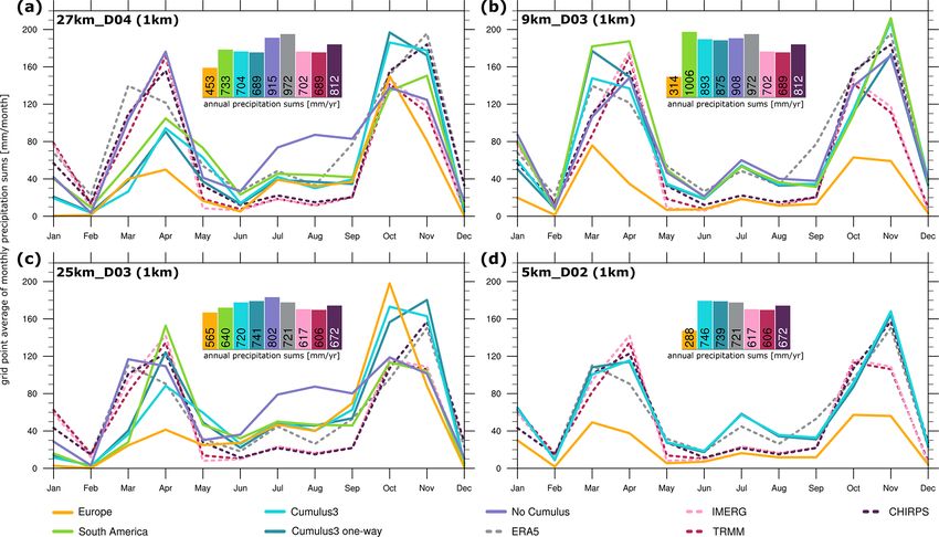
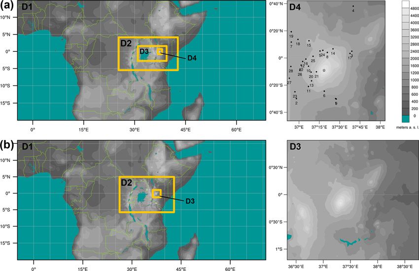
M. Messmer et al.: Sensitivity of precipitation to physics parameterizations over Mount Kenya                                  2693

lished in Stratton et al. (2018) is performed with the Met          boundary conditions provided by the reanalysis data from
Office Unified Model at 4.5 km horizontal resolution. Due           ERA5. Furthermore, the different observation-based gridded
to its high spatial resolution, it is convection-permitting, and    data for precipitation and temperature and the weather station
hence a cumulus parameterization is not needed. This sim-           data are presented in Sect. 2. Section 3 provides an analy-
ulation is investigated in more detail in Finney et al. (2019)      sis of the temporal and spatial representation of precipitation
with respect to East African climate and compared to a pa-          patterns over the area around Mount Kenya. In addition, the
rameterized 25 km spatial resolution simulation. They found         sensitivity of the different parameterization options to precip-
that the diurnal cycle in rainfall especially benefits from the     itation amounts and patterns are investigated. The analysis is
convection-permitting resolution but that precipitation inten-      topped off with a brief description of the 2 m temperature
sities and patterns also improve. Additionally, Woodhams            around Mount Kenya. Finally, the paper is wrapped up by
et al. (2018) confirmed that a convection-permitting simu-          summarizing and concluding remarks in Sect. 4.
lation is able to better represent the sub-daily precipitation
intensities over Lake Victoria and the occurrence of storms
over land. Another recent climate simulation at convection-         2     Model configuration and data
permitting scales using WRF (reaching 800 m in the inner-
most domain) was used to establish the relationship between         2.1    WRF Model
local atmospheric conditions over Kilimanjaro and the El
Niño–Southern Oscillation and Indian Ocean zonal mode               We adopt the numerical weather prediction model WRF (ver-
(Collier et al., 2018).                                             sion 3.8.1; Skamarock et al., 2008) to obtain fine-scale and
   The studies presented above already indicate that there are      local precipitation patterns. This model allows us to dynam-
several regional climate models (RCMs) available. Each of           ically downscale initial and boundary conditions, which in
these models have different sets of parameterizations that          this study are provided by ERA5 reanalysis. To determine an
can be chosen, and the ability to simulate the climate over         optimal setup for Kenya, and the Mount Kenya area in partic-
a certain region depends in large part on the selection of          ular, we test different parameterization schemes, focusing on
the different parameterization options. Several studies have        cumulus parameterizations, with two different model setups
evaluated the transferable skills of RCMs in different regions      and nesting ratios. The experiments are described in more
(e.g. Takle et al., 2007; Jacob et al., 2007; Rockel and Geyer,     detail in the following and are summarized in Table 1. The
2008; Jacob et al., 2012; Bellprat et al., 2016; Russo et al.,      experiments are all run for the same period of time, i.e. the
2019). A recent study by Russo et al. (2020) shows that the         year 2008, except for a single experiment that is repeated for
parameterization setting depends on the region of interest.         the year 2006 to evaluate the robustness of the results for
Thus, there is a need to retune RCMs for different regions.         2008 under different climate conditions. To permit the soil
Hence, this study presents a set of sensitivity studies per-        and the atmosphere to adjust to the initial conditions, we al-
formed by WRF and initiated and driven by ERA5 to find              low for 2 months of spin-up. Since the soil variables are well
an optimal setting for the representation of precipitation in       equilibrated in the ERA5 data, the used spin-up time of 2
convection-permitting simulations over Mount Kenya.                 months in our simulations is enough to bring the soil and the
   In this paper, the focus on Mount Kenya is chosen, as it         atmosphere into an equilibrium. Previous studies (Angevine
plays a crucial role in the supply of freshwater both in the        et al., 2014; Jerez et al., 2020; Velasquez et al., 2020) back up
highlands and in the surrounding lowlands (Liniger et al.,          the idea that rather short spin-up periods are enough for vari-
2005). The availability of fresh water decreases drastically        ables such as temperature or precipitation to reach the equi-
with longer distances from Mount Kenya and is further re-           librium in WRF, but for soil moisture longer periods are rec-
duced by evapotranspiration from the vegetation in the drier        ommended (a few months). This means that the simulations
savannas of the lowlands (Ngigi et al., 2007). Population           start on 1 November 2007 and end on 31 December 2008.
growth through migration puts further pressure on water                Two different nesting ratios, i.e. 1 : 3 and 1 : 5, have been
availability (Ngigi et al., 2007), which may result in disputes,    used in different model domain settings to estimate the effect
marginalization, and conflicts (Wiesmann et al., 2000). This        of the nesting ratio on the modelled precipitation and temper-
situation is exacerbated by progressive climate change that         ature (see Fig. 1). For the nesting ratio of 1 : 3, a four-domain
will affect water availability through changes in precipitation     (i.e. 27, 9, 3, 1 km horizontal resolution) and a three-domain
amounts and patterns, induced by either local or large-scale        (i.e. 9, 3, 1 km horizontal resolution) setup have been tested.
changes. To understand the behaviour of precipitation in this       In addition, the 1 : 5 nesting ratio is run with two different
complex topographical area and to obtain possible adaptation        setups, i.e. a three-nested (25, 5, 1 km horizontal resolution)
strategies, it is vital to create reliable regional climate simu-   and two-nested domain setup (5, 1 km horizontal resolution).
lations that can also be used for climate projections in a next     To test if the coarser setups affect the representation of pre-
step.                                                               cipitation and temperature over the study area, simulations
   The paper gives a detailed description of the sensitivity        with a coarser and finer parent grid are performed. This is
simulations performed with WRF, as well as its initial and          because for the coarser setups the downscaling resolution is

https://doi.org/10.5194/gmd-14-2691-2021                                              Geosci. Model Dev., 14, 2691–2711, 2021
2694                                       M. Messmer et al.: Sensitivity of precipitation to physics parameterizations over Mount Kenya

Table 1. Experimental design of the sensitivity simulations: name of the experiment, parameterizations used, and other parameters important
for each experiment, such as nesting option and ratio, number of domains, the spatial resolution of the used domains, and their corresponding
names as they appear in Fig. 1. Domains written in bold indicate that the according cumulus parameterization is turned on, while domains
printed in normal fonts do not parameterize cumulus processes. The last column provides the name of the innermost domain, which is used
in figures to identify nesting and resolution options. All other options used for the simulation can be found in the namelist files on Zenodo
(see code and data availability section).

                                    Parameterizations                                                    Other parameters                                                           Name
 Name                     Cumulus         LW-Rad.       PBL        Nesting         Nest ratio       No. of dom           Resolutions         Doms in Fig. 1               1 km domain
                          Grell–Freitas   CAM           ACM2a      two-way         1:3              4                  27, 9, 3, 1 km        (a) D1, D2, D3, D4              27km_D04
 Europe

                          Grell–Freitas   CAM           ACM2       two-way         1:3              3                      9, 3, 1 km        (a) D2, D3, D4                   9km_D03
                          Grell–Freitas   CAM           ACM2       two-way         1:5              3                    25, 5, 1 km         (b) D1, D2, D3                  25km_D03
                          –               CAM           ACM2       two-way         1:5              2                         5, 1 km        (b) D2, D3                       5km_D02
                          Kain–Fritsch    RRTMb         YSUc       two-way         1:3              4                  27, 9, 3, 1 km        (a) D1, D2, D3, D4              27km_D04
                America
  South

                          Kain–Fritsch    RRTM          YSU        two-way         1:3              3                      9, 3, 1 km        (a) D2, D3, D4                   9km_D03
                          Kain–Fritsch    RRTM          YSU        two-way         1:5              3                    25, 5, 1 km         (b) D1, D2, D3                  25km_D03
                          –               RRTM          YSU        two-way         1:5              2                         5, 1 km        (b) D2, D3                      5km_D02d
                          Grell–Freitas   RRTM          YSU        two-way         1:3              4                  27, 9, 3, 1 km        (a) D1, D2, D3, D4              27km_D04
  Cumulus3

                          Grell–Freitas   RRTM          YSU        two-way         1:3              3                      9, 3, 1 km        (a) D2, D3, D4                   9km_D03
                          Grell–Freitas   RRTM          YSU        two-way         1:5              3                    25, 5, 1 km         (b) D1, D2, D3                  25km_D03
                          –               RRTM          YSU        two-way         1:5              2                         5, 1 km        (b) D2, D3                       5km_D02
                          Grell–Freitas   RRTM          YSU        one-way         1:3              4                  27, 9, 3, 1 km        (a) D1, D2, D3, D4              27km_D04
  Cumulus3
               one-way

                          Grell–Freitas   RRTM          YSU        one-way         1:3              3                      9, 3, 1 km        (a) D2, D3, D4                   9km_D03
                          Grell–Freitas   RRTM          YSU        one-way         1:5              3                    25, 5, 1 km         (b) D1, D2, D3                  25km_D03
                          –               RRTM          YSU        one-way         1:5              2                         5, 1 km        (b) D2, D3                       5km_D02
  No cumulus

                          –               RRTM          YSU        one-way         1:3              4                  27, 9, 3, 1 km        (a) D1, D2, D3, D4              27km_D04
                          –               RRTM          YSU        one-way         1:3              3                      9, 3, 1 km        (a) D2, D3, D4                   9km_D03
                          –               RRTM          YSU        one-way         1:5              3                    25, 5, 1 km         (b) D1, D2, D3                  25km_D03
                          –               RRTM          YSU        one-way         1:5              2                         5, 1 km        (b) D2, D3                      5km_D02e
a Asymmetric Convection Model Version2. b Rapid Radiative Transfer Model. c Yonsei University. d This simulation is identical to the last one in “Cumulus3” and therefore it is only
shown related to the Cumulus3 parameterization option in Figs. 3, 4, and 5; e This simulation is identical to the last one in “Cumulus3 one-way”, and therefore it is only shown related
to the Cumulus3 one-way parameterization option in Figs. 3, 4, and 5.

very similar to the one of ERA5, which provides the initial                                       750 s for the 1 : 5 ratio. For the smaller domains, the time
and boundary conditions. Such coarse spatial resolutions in                                       steps are reduced by the factor of the nesting ratio. A small
the outermost domains are tested because the final goal is to                                     sensitivity test, starting the simulation twice from the same
also apply the WRF setup to climate simulations, which nor-                                       restart file, indicates that the simulation is also reproducible
mally have a coarser resolution (around 100 km) than reanal-                                      with an adaptive time step.
ysis data (around 30 km for ERA5). In that case, a climate                                           Different physical parameterization schemes have been
simulation with a parent domain starting at 9 or 5 km is not                                      tested to optimize the representation of precipitation over
possible. Nevertheless, the parameterizations are tested using                                    Kenya. Tests have been done by varying the cumulus, the
ERA5 as boundary condition in order to be able to compare                                         longwave (LW) radiation, and the planetary boundary layer
the simulations against observations of the year 2008. Note                                       (PBL) parameterization schemes. For cumulus parameteri-
that in the simulations with a reduced number of nests (three                                     zation, the Kain–Fritsch (Kain, 2004) and the scale-aware
domains instead of four for the 1 : 3 ratio, and two instead                                      Grell–Freitas ensemble (Grell and Freitas, 2014) schemes
of three for the 1 : 5 ratio), the parent domain always corre-                                    have been used in the domains with resolutions > 5 km, and
sponds to the second domain of the experiment with one nest                                       one experiment is performed without using any cumulus pa-
more (Table 1). All simulations have 49 vertical eta levels                                       rameterization in all of the domains. Note that the cumulus
up to 50 hPa and an innermost domain located over Mount                                           parameterization is switched off in all experiments for do-
Kenya with 1 km horizontal resolution. When comparing the                                         mains with horizontal resolutions ≤ 5 km. The LW radiation
different sensitivity experiments in the results (Sect. 3), the                                   scheme has been varied between the Rapid Radiation Trans-
focus is always on the innermost domain of all the simula-                                        fer Model (RRTM; Mlawer et al., 1997) and Community At-
tions. To save some computational costs, an adaptive time                                         mosphere Model (CAM; Collins et al., 2004). The two first-
step is used, which is between 54 and 810 s in the outermost                                      order non-local-closure PBL schemes of Yonsei University
domain for the 1 : 3 ratio experiments and between 50 and                                         (Hong et al., 2006) and the second version of the Asym-

Geosci. Model Dev., 14, 2691–2711, 2021                                                                                    https://doi.org/10.5194/gmd-14-2691-2021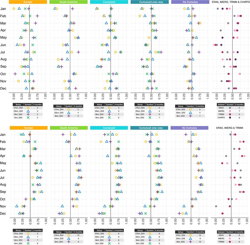
M. Messmer et al.: Sensitivity of precipitation to physics parameterizations over Mount Kenya                                         2695

Figure 1. The two different nesting settings for the sensitivity experiments are depicted. The four domains (D1 = 27 km, D2 = 9 km,
D3 = 3 km, D4 = 1 km) of the nesting ratio 1 : 3 are shown in row (a), with the topography of the innermost nest D4 in the right panel.
The three domains (D1 = 25 km, D2 = 5 km, D3 = 1 km) of the nesting ratio 1 : 5 are shown in row (b), with the topography of the innermost
nest D3 in the right panel. The grey shading indicates elevation in metres above sea level using the WRF topography Global Multi-resolution
Terrain Elevation Data (GMTED2010) provided by USGS. The location of the weather station data is provided in D4, and a more detailed
description of each station is available in Table 2. The black star in D4 indicates the summit of Mount Kenya. Note that at least 30 grid
points from the edge of the boundaries of an inner domain to the limit of an outer domain are used to avoid effects from the relaxation zone
(spanning five grid points) between two nests (Rummukainen, 2010).

metric Convection Model (Pleim, 2007) have been tested.                 tive effects and thus precipitation over the lake and in the sur-
Table 1 provides a summary of the used parameterizations                rounding areas. A comparison of one simulation with the lake
for each experiment and the exact setting can be found in               model turned off and one including the lake model reveals
the namelist files on Zenodo (see the code and data avail-              that the lake model is slightly beneficial for representing tem-
ability section). The rest of the parameterization options are          poral and spatial precipitation patterns around Mount Kenya.
kept constant throughout the different experiments, i.e. WRF            Hence, the experiment without lake model is not presented in
single-moment 6-class scheme (Hong and Lim, 2006) for mi-               the following analysis. Please note that the aforementioned
crophysics, Dudhia shortwave (SW) scheme for the SW radi-               parameterization options are selected from an even larger set
ation (Dudhia, 1988), and the Noah–MP land surface model                of experiments not included in this paper and are only tested
(Niu et al., 2011; Yang et al., 2011) to describe surface pro-          with one nesting ratio and four nested domains. In addition,
cesses. In all the simulations the lake model is turned on. The         a simulation with the latest version of the model (V4.2.1)
1-D physically based lake model (Subin et al., 2012) helps to           was run. However, it showed that the included improvements
simulate lake internal processes and interactions at the sur-           are not enough to reduce the root-mean-square error (RMSE)
face of the lake with the atmosphere (Gu et al., 2015). It in-          and to improve the temporal correlation against the weather
creases the eddy diffusivity, and it thus also strengthens the          station data compared to the other sets of experiments. It fur-
heat transfer in the lake column (Gu et al., 2015). This is con-        ther indicates that model versions and compilers can impact
sidered to be beneficial for the description of the lake surface        the simulations performed with WRF. Consequently, it has
temperature, which again helps to better represent evapora-             not been included in the analysis presented here.

https://doi.org/10.5194/gmd-14-2691-2021                                                    Geosci. Model Dev., 14, 2691–2711, 2021
2696 M. Messmer et al.: Sensitivity of precipitation to physics parameterizations over Mount Kenya
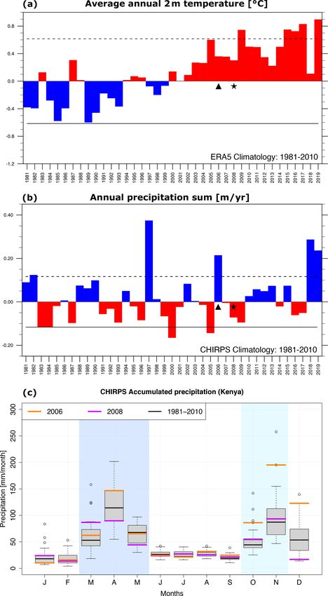
As already shown in Table 1, each experiment obtained a matology of Kenya for the year 1981–2010, the year 2008 is
name, chosen based on the area used in the literature or on one of the warmer years, but when considering the constant
the main parameterization that it employs. The “Europe” ex- warming since the beginning of the current millennium, it
periment is based on the parameterization options used with can be considered as a new normal (Fig. 2a). The analysis of
WRF over Europe in previous studies by the authors (Mess- the detrended data also supports this (not shown). In terms
mer et al., 2017) but also including some updated schemes of precipitation, 2008 is on the dry side compared to the cli-
such as the Noah-MP land surface model. “South America” matology (Fig. 2b), but it is a year with two clear rainy sea-
is based on the parameterizations used for the optimal sim- sons, the long rains, and the short rains (Fig. 2c). Addition-
ulation of storms over the central Andes (Zamuriano et al., ally, the year 2006 is selected as it is rather wet compared to
2019). The remaining “Cumulus” experiments are similar the year 2008.
to the configurations applied over East Africa in previous
studies (Pohl et al., 2011; Otieno et al., 2019), but they in- 2.3 Observational data sets
clude the updated Noah-MP land surface model and changes
in the cumulus scheme option (option 3 in WRF – “Cumu- To analyse the output of the WRF simulations and to identify
lus3” experiment) or no use of cumulus parameterizations at the best parameterization options, the downscaled product
all (“No Cumulus”). The No Cumulus experiment is moti- must be compared to some independent observational data
vated by a recent study (Vergara-Temprado et al., 2020) that sets. Hence, the precipitation results are compared to ERA5,
shows some improvements in resolving convective precipita- three satellite-based data sets and independent weather sta-
tion explicitly compared to parameterized convection in hor- tion measurements. For temperature, the results are com-
izontal resolutions of around 25 km. The difference between pared to ERA5. A comparison to the temperature data of Cli-
the Cumulus3 and “Cumulus3 one-way” is the communica- matic Research Unit (CRU) data has also been performed,
tion between the parent and the respective child nest. In the but the patterns are very similar to ERA5 and are there-
one-way nested options, results from the inner domain are fore not shown here. Please note that the gridded data sets
not overwritten on the parent grid, while this is the case for are bilinearly interpolated (Climate Data Operator (CDO);
two-way nested domains. Note that the two-domain simu- Schulzweida, 2019) to the grid of the WRF domain that it is
lation starting at 5 km horizontal resolution is equal for the compared to, and the nearest point to the station is consid-
Cumulus3 one-way and the No Cumulus experiment, as they ered afterwards. Consequently, small differences can appear
differ only in the cumulus parameterization. As both in that in the values related to the gridded observational data sets.
particular simulation explicitly resolve convective processes, However, when the pattern correlation is calculated against
the simulations are identical and will be presented as Cumu- gridded data sets, the grid of this data set is taken as a ref-
lus3 one-way. This is also the case for the experiments South erence, and the WRF simulations are bilinearly interpolated
America and Cumulus3, as they both explicitly resolve con- to that grid. In the following, the different products are de-
vective processes in simulations starting at 5 km horizontal scribed in more detail.
resolution. Thus, both experiments are also identical and will
be presented as Cumulus3. 2.3.1 Tropical Rainfall Measurement Mission (TRMM)
2.2 ERA5 The Tropical Rainfall Measurement Mission (TRMM) com-
prises several data sets based on satellite data, and it is pro-
ERA5 is the latest reanalysis provided by the European Cen- vided by NASA and the Japanese Aerospace Exploration
tre for Medium-Range Weather Forecasts (ECMWF). At the Agency (JAXA). In this study we use the gridded data prod-
moment, it is available from January 1979 until 3 months uct TRMM 3B42 for precipitation estimates. Note that we
before present (Copernicus Climate Change Service, 2017). use the research-grade TRMM 3B42 and not the near-real-
ERA5 provides different variables on the surface and vari- time version, as the first is considered to be more suitable
ous pressure levels with an hourly output. Nevertheless, we for research (Liu, 2015). Version 7 of TRMM 3B42 (TMPA
use 6-hourly data for our boundary conditions. The data are 3B42 v7) is a combined product and merges satellite rainfall
available globally on a 0.25◦ horizontal grid spacing and use estimates with gauge data. To obtain the 3-hourly precipi-
137 vertical model levels. A vast number of observations and tation estimates, radars are calibrated to the microwave im-
satellite data are assimilated to the ERA5 gridded data us- ager precipitation, which should result in a 3 h microwave-
ing the integrated forecasting system cycle 41r2. A total of only best estimate. In a next step, infrared precipitation is
24 vertical pressure levels were fed to WRF (1000, 925, 900, calibrated to the microwave product to fill regional gaps. Fi-
850, 800, 775, 750, 700, 650, 600, 550, 500, 450, 400, 350, nally, the 3-hourly estimate is summed up to monthly val-
300, 250, 200, 150, 100, 50, 30, 20, 10 hPa). ues and recalibrated using a rain gauge analysis (Huffman
As stated before, our analysis will focus only on the et al., 2007, 2010). This monthly surface precipitation gauge
year 2008, although 2006 is used to test the performance of analysis is obtained from the Global Precipitation Climatol-
the best setting using a different year. Compared to the cli- ogy Centre (GPCC). The result is a Level-3 product with
Geosci. Model Dev., 14, 2691–2711, 2021 https://doi.org/10.5194/gmd-14-2691-2021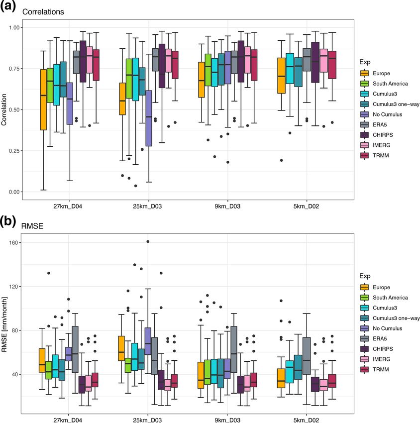
M. Messmer et al.: Sensitivity of precipitation to physics parameterizations over Mount Kenya                                       2697

                                                                         3-hourly temporal and 0.25◦ × 0.25◦ spatial resolution on
                                                                         a quasi-global (50◦ N–50◦ S) grid. With this resolution the
                                                                         TRMM 3B42 data is very similar to ERA5. TRMM 3B42 is
                                                                         available for the period 29 February 2000 to 2 January 2020.

                                                                         2.3.2   IMERG

                                                                         The Integrated Multi-satellitE Retrievals from GPM
                                                                         (IMERG) provides a multi-satellite product, currently avail-
                                                                         able in its sixth version. It is the successor to the TRMM
                                                                         data set. Several products with different latency periods
                                                                         are available, but for this study we make use of the final
                                                                         product, which is suitable for scientific purposes. Similar
                                                                         to TRMM, several microwave measurements are used to
                                                                         estimate precipitation, and it is further calibrated against
                                                                         instrument products. The half-hourly precipitation estimates
                                                                         are further recalibrated with a CMORPH Kalman filter and
                                                                         the PERSIANN Cloud Classification System artificial neural
                                                                         network. The product is finally adjusted to the monthly
                                                                         GPCC rain gauge measurements and is available in half-
                                                                         hourly time steps and on a spatial resolution of 0.1◦ × 0.1◦
                                                                         (approximately 10 km × 10 km). The available time period
                                                                         is from June 2000 until present.

                                                                         2.3.3   CHIRPS

                                                                         The Climate Hazards group Infrared Precipitation with Sta-
                                                                         tions (CHIRPS V2.0) provides a high-resolution data set with
                                                                         daily rainfall amounts (Funk et al., 2015). The 0.05◦ spa-
                                                                         tially resolved data are available for parts of the mid-latitudes
                                                                         and the tropics (50◦ S–50◦ N). The data set is generated us-
                                                                         ing thermal infrared precipitation products from different in-
                                                                         stitutions. To calibrate global cold cloud duration rainfall
                                                                         estimates, the Tropical Rainfall Measuring Mission Multi-
                                                                         satellite Precipitation Analysis version 7 (TMPA 3B42 v7)
                                                                         is used (Funk et al., 2015). In a first step, the World Meteo-
                                                                         rological Organization’s Global Telecommunications System
                                                                         (GTS) rain gauge data, which are relatively sparsely avail-
                                                                         able, are combined with cold cloud-duration-derived precip-
                                                                         itation estimates. In a second step, the best available weather
Figure 2. Annual anomalies of mean 2 m temperature (in ◦ C) from
                                                                         station data are combined with cold cloud-duration-based
ERA5 (Copernicus Climate Change Service, 2017) (a) and of pre-
cipitation (in metres per year) from CHIRPS (Funk et al., 2015) (b).
                                                                         precipitation to get a product that on a monthly mean is simi-
The anomalies are calculated with respect to the climatological          lar to those produced by the GPCC or the CRU from the Uni-
mean of the years 1981 to 2010. The stippled (straight) lines il-        versity of East Anglia (Funk et al., 2015). Note that IMERG
lustrate plus (minus) 1 standard deviation. Monthly accumulated          and TRMM also recalibrate their monthly output to results
values of precipitation (in millimetres per month) for the selected      obtained from GPCC, and CHIRPS is based on the same
year 2008 (in purple) and 2006 (in orange) compared to the cli-          satellite product as TRMM, hence the three data sets used
matology (1981–2010, in grey, using a box and whisker plot) are          for the model verification are not fully independent of each
shown in (c). All values are means over the territory of Kenya in        other, especially when monthly sums are investigated.
each subplot. The whiskers extend to the value that is no more than
1.5 times the interquartile range away from the box. The values out-
side this range are defined as outliers and are plotted with dots. The
dark blue and light blue shading indicate the long rains and short
rains, respectively.

https://doi.org/10.5194/gmd-14-2691-2021                                                   Geosci. Model Dev., 14, 2691–2711, 2021
2698 M. Messmer et al.: Sensitivity of precipitation to physics parameterizations over Mount Kenya
2.3.4 Weather station data gridded observational data sets are compared to in situ data
from weather stations (see Table 2 for more details). To com-
Compared to other tropical areas in Africa, Kenya (and es- pare gridded data with point measurements at weather sta-
pecially the area around Mount Kenya) is covered by a com- tions, the grid point that is closest to the corresponding lati-
parably large number of weather station data with long pre- tude and longitude of the weather station is considered in the
cipitation measurement series. Many of these measurement WRF simulation and the gridded observations. Two perfor-
series are maintained by farmers. Thanks to the support and mance measures for each weather station are calculated and
involvement of the University of Nairobi and University of summarized in box and whisker plots (Fig. 3): the temporal
Bern, these series are still available today (Gichuki et al., correlation and the RMSE. For correlations we use the Spear-
1998; Liniger et al., 2005; MacMillan and Liniger, 2005). man correlation, which is a rank correlation that is suitable
In addition to private stations, there are also some that are for the small sample sizes that are explored here. Addition-
operated by the government of Kenya, i.e. the Kenya Forest ally, the standard deviation of each data set is compared to the
Service or the Kenyan Meteorological Department. For pre- one extracted from the weather stations (not shown). Several
cipitation, we use data from 28 stations that have been qual- different gridded observational data sets are employed here
ity controlled by Schmocker et al. (2016). Table 2 provides to compare the sensitivity simulations and to classify which
some information on the stations used in this study, but for WRF setting performs best. As not only the weather station
more detailed information the reader is referred to Table 1 data but also the gridded observational data sets are subject
in Schmocker et al. (2016). The station ID in both tables to a range of uncertainties, we rely on more than one prod-
are identical to ease comparison. We obtained four stations uct. Note that because the gridded data sets are bilinearly in-
with temperature records from the Social Hydrological In- terpolated to the respective WRF grid, small differences can
formation Platform (SHIP), which is associated with the Wa- appear in the values of temporal correlations and RMSEs of
ter and Land Resources Centre (WLRC) project of the Cen- each setup, and hence the shape of bars corresponding to
tre for Training and Integrated Research In ASAL Develop- these data sets in the box and whisker plots can also look
ment (CETRAD). Three additional stations for precipitation slightly different.
and temperature are included in the World Weather Records The temporal correlations show that the observational data
(WWR) database from the World Meteorological Organiza- sets (ERA5, TRMM, and especially IMERG) are well corre-
tion (WMO). These are the three first lines of Table 2. Note lated (Fig. 3a). This is expected as the data are not fully in-
that the weather station data have not been adjusted to the dependent from each other. IMERG has the best correlation
height of the model topography, as the differences in height with the highest median but also with the smallest spread.
are in the range of a few metres. The maximum difference Generally, the observational datasets show a good correlation
between the station and model height is around 60 m, and of around 0.8 in the median value. The fact that IMERG and
hence the maximum discrepancy between station and mod- the weather station data show such a good agreement further
elled temperature is around 0.4 ◦ C if we consider the standard confirms the quality of the latter. The temporal correlations of
environmental lapse rate of 6.5 K km−1 (Barry, 2008). Addi- the sensitivity simulations show a strong dependence on the
tionally, the quality control performed by Schmocker et al. nesting options. The simulations with fewer nests (right part
(2016) suggests that several stations are only suitable for of Fig. 3a) exhibit a higher correlation and a smaller spread
monthly analyses. As the number of stations in the innermost than the two simulations that have one additional nest (left
domain should stay as large as possible, the study is mainly part of Fig. 3a). In particular, the No Cumulus simulation
based on the monthly resolution. Most of the weather stations and the Europe setup show a poor performance in the tem-
are located on the northwestern slopes of Mount Kenya, and poral correlation. Note that the poor performance of the No
they are rather scarce to the southeast of it, which could affect Cumulus setup can only be observed in nesting options with
the reliability of our results. However, we reduce this uncer- a larger number of domains, i.e. setups with a parent grid of
tainty by also comparing our results against several gridded 27 or 25 km. The fact that the nesting option is important here
observational data sets. suggests that with fewer domains (only three instead of four
nests for the 1 : 3 ratio and two instead of three for the 1 : 5
ratio), the simulation in the innermost domain is still more
3 Results
strongly influenced by the boundary conditions of the driv-
3.1 Sensitivity of precipitation ing data, i.e. ERA5. Thus, the simulations with fewer nests
cannot evolve with the same freedom as the ones with more
3.1.1 Temporal analysis nests, resulting in a better temporal agreement of the simula-
tions. This is especially clear in the No Cumulus simulation.
To investigate the sensitivity of simulated precipitation due While all the gridded observational data sets yield a rather
to different parameterization options of the WRF model, high temporal correlation, the RMSE of ERA5 is rather
we first show the annual cycle based on monthly means. high compared to the ones of TRMM, IMERG and CHIRPS
Thereby, the sensitivity simulations with WRF and the three (Fig. 3b). A reason for this is that the precipitation in ERA5
Geosci. Model Dev., 14, 2691–2711, 2021 https://doi.org/10.5194/gmd-14-2691-2021M. Messmer et al.: Sensitivity of precipitation to physics parameterizations over Mount Kenya 2699
Table 2. Weather station information: station number used in our study (labels in Figs. 1, 6, and 7), station name, location (latitude and
longitude), altitude (in metres above sea level), number of missing values, variables available, and station ID from WMO (first three lines)
or from Table 1 in Schmocker et al. (2016). RR stands for precipitation and T2 for 2 m temperature.
Number Station Lat Long Altitude [m] No. missing Variable ID
1 Embu WMO −0.5 37.45 1493 0 RR, T2 637200
2 Nyeri WMO −0.5 36.967 1759 0 RR, T2 637170
3 Meru WMO 0.083 37.65 1554 0 RR, T2 636950
4 Archers Post 0.6375 37.6675 839 0 RR, T2 1
5 Ardencaple Farm 0.0852 37.258 2271 0 RR 2
6 Castle Forest Station −0.4083 37.3107 1927 0 RR 5
7 El Karama 0.1952 36.9038 1781 0 RR 95
8 Embori Farm 0.0677 37.3482 2691 0 RR 12
9 Embu Met Station −0.5047 37.4579 1743 0 RR 14
10 Gathiuru Forest Station −0.1018 37.1159 2333 0 RR 17
11 Hombe Forest Station −0.3508 37.1158 2017 0 RR 20
12 Jacobson Farm −0.0432 37.0444 1913 0 RR 23
13 Kabaru Forest Station −0.2814 37.1535 2279 0 RR 25
14 Kisima Farm 0.1118 37.4181 2465 0 RR 35
15 Loldaiga Farm 0.2117 37.1219 2135 0 RR 34
16 Loruku Farm −0.0136 37.0839 1896 0 RR 38
17 Meru Forest Station 0.0557 37.6277 1737 0 RR 45
18 Mogwoni Ranch 0.2284 36.9862 1683 0 RR 47
19 Mpala Farm 0.3227 36.9038 1844 0 RR 48
20 Naro Moru Gate Station −0.1744 37.148 2471 0 RR 61
21 Naro Moru Met Station −0.1704 37.214 3048 0 RR, T2 62
22 Nicholson Farm −0.0886 37.0259 1916 0 RR 66
23 Nyeri Mow −0.4162 36.9489 1854 92 RR 67
24 Ol Donyo Farm 0.0938 37.2929 2375 0 RR 69
25 Ontulili Forest Station 0.0206 37.1723 2056 0 RR 75
26 Satima Farm −0.1475 37.0101 1944 0 RR 82
27 Solio Ranch −0.2493 36.8797 1943 0 RR 87
28 Tharua Farm −0.1046 36.8985 1865 0 RR 92
29 Kalalu 0.0817 37.1638 2027 0 T2 –
30 Munyaka -0.1833 37.0596 2048 0 T2 –
is independent of the weather station data, as precipitation leads to a general reduction of the correlation coefficients and
is not assimilated into this product. Otherwise, the RMSE an increase in RMSEs. This is expected, as the variability
shows similar results to the correlations for both the grid- is higher and because it is more and more challenging for
ded observations and the sensitivity simulations. Hence, the the model to capture the exact timing of precipitation (not
parameterization of the simulation is only of minor impor- shown).
tance compared to the nesting options. Similar findings are
obtained when using the standard deviation (not shown). 3.1.2 Pattern correlation analysis
Here, the WRF simulations are generally within the range of
the standard deviation observed in the weather station data, Since the temporal correlation and the RMSE do not clearly
except for the Europe parameterization in the nesting op- define which parameterization option of WRF delivers the
tions with fewer nests. In that case, the standard deviation best results for precipitation in the region around Mount
is strongly underestimated, indicating that the variability of Kenya, we investigate the pattern correlation of the simula-
precipitation is not fully captured. Additionally, the standard tions compared to weather station data in a first step and to
deviations of the gridded observational data sets are smaller the gridded observational data set CHIRPS in a second step.
than the ones of the weather station data, which is owed to the Figure 4 shows the pattern correlation between the WRF-
coarser resolution of the first. At finer temporal resolutions simulations and the weather station data for each month in
than monthly sums, these temporal correlations and RMSEs the first row. The different columns indicate different param-
reproduce the differences between the experiments as dis- eterization options, and the symbols within each panel show
cussed for monthly means. However, using finer timescales the nesting option. The vertical black line in each panel is
equal to a correlation coefficient of 0.5. This value is a mod-
https://doi.org/10.5194/gmd-14-2691-2021 Geosci. Model Dev., 14, 2691–2711, 20212700 M. Messmer et al.: Sensitivity of precipitation to physics parameterizations over Mount Kenya Figure 3. The temporal correlation (a) and root-mean-square error (RMSE) (b) between the annual cycle for the year 2008 of measured and simulated monthly precipitation sums at the nearest grid point to the station’s location shown for the different parameterization options (see legend to the right, Table 1) and grouped by the different nesting options and number of nests. The box and whisker plots show the values in relation to 28 stations for the different domains with 1 km spatial resolution. The whiskers extend to a value that is no more than 1.5 times the interquartile range away from the box. The values outside this range are defined as outliers and are plotted with dots. erate correlation and still explains roughly 25 % of the vari- tion, the simulations with fewer nests obtain a better pattern ance, but it is a visual support to more easily determine which correlation compared to the ones with an additional nest. The simulations and nesting options perform better than others. South America and the No Cumulus parameterizations show The number of months that are equal to or exceed this limit the highest agreement with the weather station data for the of 0.5 in correlation are counted and summed up in the table nesting options that have an additional nest, while clearly below each panel (“# months” column). the Cumulus3 one-way option is the best of the simulations The gridded observational data sets agree reasonably well with fewer nests. Overall, the simulations have a better per- in terms of the spatial pattern of precipitation, except for formance in the rainy seasons MAM and ON, while the dry ERA5. The fact that ERA5 shows a poor correlation with months (and June in particular) are not very well captured by the weather station data is because the domain is located the model simulations. over steep terrain, where a high resolution is needed to re- Besides the comparison to the weather station data, the solve precipitation patterns appropriately. CHIRPS has the simulations and gridded observational data are compared to highest spatial resolution and shows a slightly better pattern CHIRPS (see the second row of Fig. 4). As mentioned be- correlation than IMERG (especially in June), and hence we fore, all the simulations were bilinearly interpolated to the have decided to also compare the WRF simulations against grid of CHIRPS for this spatial analysis. The gridded ob- the CHIRPS gridded data set (second row of Fig. 4). Addi- servational data sets perform well compared to CHIRPS (in- tionally, CHIRPS shows high correlations and low RMSEs cluding ERA5). Again this is expected as the data are not in the temporal analysis. Similarly to the temporal correla- fully independent. The pattern correlation of the WRF sim- Geosci. Model Dev., 14, 2691–2711, 2021 https://doi.org/10.5194/gmd-14-2691-2021
M. Messmer et al.: Sensitivity of precipitation to physics parameterizations over Mount Kenya                                             2701

Figure 4. Pattern correlation of monthly precipitation sums for the year 2008 between weather station data and the respective WRF simulation
(upper row) and between CHIRPS and the respective WRF simulation (interpolated onto the CHIRPS grid, lower row). The different panels
indicate the different parameterization options (Table 1), and the symbols stand for the different nesting options. The labelling of the symbols
is given in the table below each panel, along with the number of months (# months) in which the nesting option obtain correlation patterns
above the reference value of 0.50 (a moderate correlation used to visually evaluate the performance of nesting options). The last panel on
each row represents the gridded data sets used throughout the paper. Even if the gridded data sets are interpolated onto different domains for
each independent setup, here only one setting is shown (27km_D04, only first row). The rest was omitted as only marginal changes can be
observed.

ulations compared to CHIRPS are rather high in all the sim-               The Europe parameterization is clearly the worst, even if it
ulations. No clear difference between the different nesting               shows one of the highest correlations in the dry months of
options are evident. The South America and the No Cumulus                 June and July. This is because the Europe parameterization
options show the best agreement with CHIRPS in precipi-                   setup produces rather dry conditions over Africa, and hence
tation patterns, but Cumulus3 one-way also performs well.

https://doi.org/10.5194/gmd-14-2691-2021                                                       Geosci. Model Dev., 14, 2691–2711, 2021
2702 M. Messmer et al.: Sensitivity of precipitation to physics parameterizations over Mount Kenya
the dry months are better represented compared to the others precipitation, and hence it clearly underestimates the water
that simulate generally wetter conditions. availability. All the other settings perform similarly well on
an annual basis (insets in Fig. 5). It is also noteworthy that the
3.1.3 Annual cycle WRF model with the Cumulus 3 options is able to correct the
overestimation obtained by ERA5, which is the driving data
To further understand how well the different parameteriza- set of the simulations.
tion and nesting options are able to represent precipitation
around Mount Kenya, the annual cycle is plotted as grid point 3.1.4 Precipitation patterns
averages of monthly precipitation sums of the innermost do-
main (1 km; Fig. 5). Please note that the gridded observa- Another measure used to identify the best setup of WRF for
tional data sets do not obtain exactly the same values for the this region is the precipitation patterns of the WRF simula-
different nesting ratios 1 : 3 (first row) and 1 : 5 (second row), tions. Due to the aforementioned motivation to use the tested
as the domain sizes are not exactly equal. The innermost do- settings in a climate simulation, in the following the simu-
main in the 1 : 5 nesting ratio setup is slightly bigger. The lation of the innermost domain (D4; 1 km) with the parent
three gridded observational data sets TRMM, IMERG, and domain of 27 km horizontal grid spacing and a nesting ra-
CHIRPS agree well and are considered the reference here be- tio of 1 : 3 is presented. Note that the simulations with a
cause they show a good temporal and pattern correlation with 25 km parent grid and a nesting ratio of 1 : 5 show similar
the weather station data. This is true except for November, results and are hence not shown here. To present the results,
when CHIRPS records a much higher value in precipitation months within the three main seasons are presented, i.e. the
amounts than TRMM and IMERG. As CHIRPS shows one long rains, short rains, and the dry season. April (Fig. 6a)
of the weakest pattern correlations in November compared is chosen as it is in the midst of the long rains. November
to the weather station data, IMERG and TRMM should be (Fig. 6b) is selected as it is within the short rains and has a
considered the reference in this month. ERA5 also agrees, larger spread between the different experiments than Octo-
but the long rains (MAM) have the peak intensity a bit too ber. Finally, June (Fig. 6c) represents a month in the dry sea-
early, while the intensity in the short rains (ON) is too in- son and shows stronger deviations compared to station data.
tense on average. For the dry months, ERA5 also overesti- As CHIRPS is the data set that shows the best agreement with
mates precipitation compared to the other gridded observa- the weather station data (as shown in Fig. 4) and because it
tional products. Overall, the gridded data sets come up with also shows the highest resolution and detail, in the follow-
similar annual precipitation sums (see the inset of Fig. 5), ing only this gridded observational data set is presented as a
except for ERA5, which shows a slight overestimation in reference. Additionally, the Europe experiment is discarded
annual precipitation sums. Comparing the monthly precipi- because of its weak performance in the previous analyses.
tation sums of the sensitivity simulations with the gridded In April, the precipitation from CHIRPS is similar to the
observational reference, we find again that the Europe pa- measured amounts of precipitation, with the exception of a
rameterization option is not well suited for this area as it small region located to the north of Mount Kenya where pre-
is not able to correctly capture the two rainy seasons near cipitation is overestimated by this gridded data set (Fig. 6a).
Mount Kenya. The long rains show a clear deficit in precipi- Bearing in mind that the observational data set is also sub-
tation, while the outcome of the short rains strongly depends ject to some uncertainties, the South America parameteriza-
on the number of nests. With fewer nests the short rains are tion shows similar precipitation amounts and patterns along
also clearly underestimated but with an additional nest pre- a diagonal band from southwest to northeast, lacking some
cipitation is either almost correct or is overestimated. The of the precipitation southeast of Mount Kenya, as indicated
differences between the Europe setup and the others are re- by CHIRPS. The northern part of the domain seems to be
lated to the parameterization of the longwave radiation and too dry compared to CHIRPS, but stations along the northern
PBL, which are both responsible for the reduction in precip- slope of Mount Kenya agree relatively well. The other three
itation amounts according to previous sensitivity tests with setups manage to produce a precipitation pattern as observed
these parameterizations (not shown). The No Cumulus setup in CHIRPS. Nevertheless, the No Cumulus parameterization
performs well in both wet seasons, but it overestimates pre- is too wet, especially in the northwestern part of the domain,
cipitation during the dry season. The Cumulus3 options show and the steep gradient from high precipitation rates in the
a clear sensitivity of the precipitation amounts in the long vicinity of Mount Kenya to dryer conditions to the northwest
rains to the number of nests, with a much better representa- of it is not well captured. The two Cumulus3 parameteriza-
tion with fewer nests. In the short rains, the Cumulus3 op- tion options capture this pattern the best, including also some
tions follow the curve of CHIRPS and therefore shows an finer details along the right and bottom boundaries of the do-
overestimation. The fact that the Europe setting is not suited main.
for this region becomes even clearer when including the an- CHIRPS also captures the precipitation pattern quite well
nual precipitation sums. Except for the 25 km parent grid, in November, with some deviations compared to the weather
the Europe setting captures only around 50 % of the annual station data south and northwest of Mount Kenya (Fig. 6b).
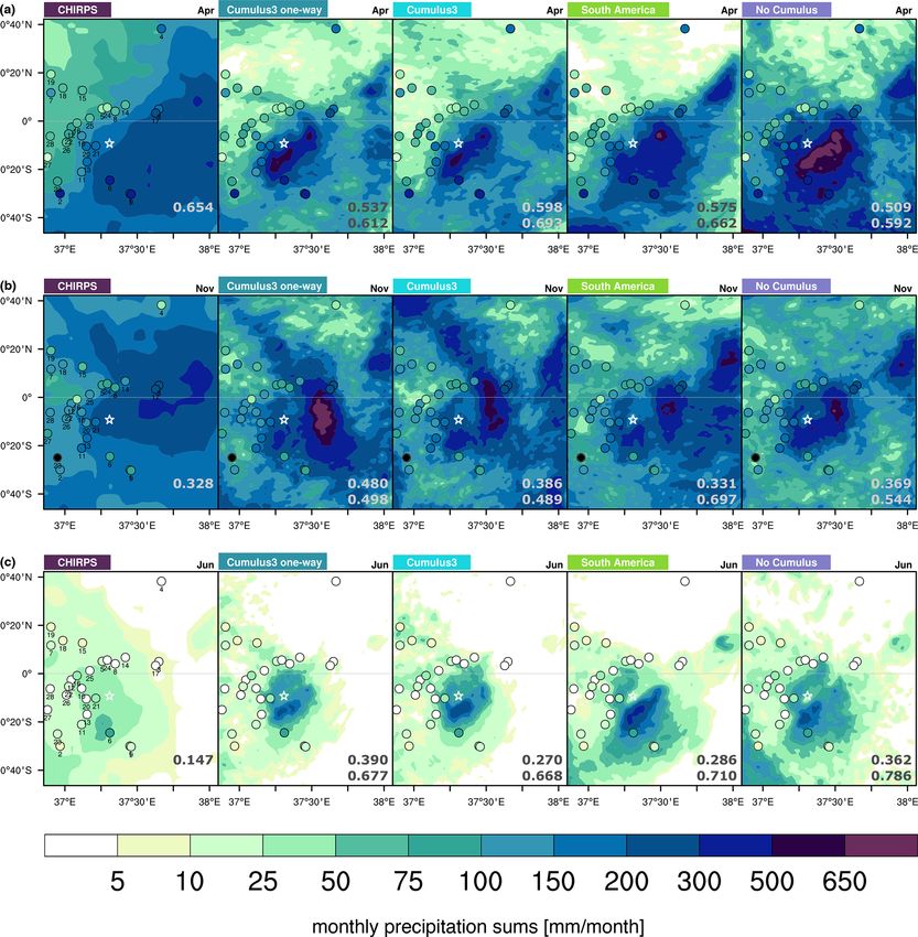
Geosci. Model Dev., 14, 2691–2711, 2021 https://doi.org/10.5194/gmd-14-2691-2021M. Messmer et al.: Sensitivity of precipitation to physics parameterizations over Mount Kenya 2703 Figure 5. Grid point averages of monthly precipitation sums in millimetres per month for the year 2008 in the innermost domain (1 km) for each of the tested setups: 27 km (a), 9 km (b), 25 km (c), and 5 km (d). The five tested parameterization options are included, along with the driving reanalysis ERA5 and the three observational gridded data sets (IMERG, TRMM, and CHIRPS). All the gridded data sets are plotted with different shades of pink, while ERA5 is coloured in grey. The inset of a bar plot in each panel indicates the grid point average annual precipitation sum in millimetres per year for each parameterization option and gridded data set. South America captures the precipitation amounts of the sta- one-way nesting does not overwrite the solution of the cor- tions quite well, but the pattern shows some deviations com- responding parent grid, this option should be preferred over pared to CHIRPS, especially in the northwestern corner of the two-way nesting option. It allows us not only to focus the domain. The two Cumulus3 and the No Cumulus op- on the innermost domain but also investigate the larger-scale tions are able to capture the patterns well with some over- picture without any disturbances within the domain. estimation in the simulations driven by the first option and a All the WRF simulations reasonably resemble the pre- slight underestimation in precipitation amounts for the latter cipitation pattern over Mount Kenya in the year 2008. The parameterization option. Given the uncertainty range within Europe setting provides the worst performance and too dry the observation-based data, it cannot be expected that a sin- conditions throughout the whole year. The No Cumulus pa- gle sensitivity simulation can agree with all the stations or rameterization and the Cumulus3 options provide the best with one of the gridded observational data sets. performances throughout the analysis. The fact that the No June is clearly much drier than April, and CHIRPS also Cumulus option is generally too wet allows us to define the records too much precipitation compared to the weather sta- Cumulus3 one-way option as the best for our purpose. Note tion data (see Fig. 6c). Given the uncertainty range of the also that the No Cumulus parameterization option produces a observation-based data, the South America parameterization patchy picture in the outermost domain with monthly sums, option does not fully agree with CHIRPS in terms of the gen- which is a clear sign of a structural problem, i.e. convec- eral pattern, as no dry corridor in the east is simulated and tion always being induced at the same location (not shown), precipitation is overestimated at most of the stations. This is which is rather unrealistic. Hence, this simulation is also un- also true for the No Cumulus parameterization option, but suitable for a larger-scale analysis of precipitation and pre- here the pattern agrees better, with a clear overestimation cipitation changes in a warmer climate. Even if we are only in precipitation amounts. Cumulus3 and Cumulus3 one-way interested in the results on a kilometre-level scale, it must be again result in the best pattern, rendering it difficult to choose noted that the timing (not necessarily the amount) of the peak between the two, as some stations are better in one setting precipitation rates on a sub-daily basis are captured more re- and other stations are better described in the other. Since alistically with respect to IMERG by the No Cumulus exper- https://doi.org/10.5194/gmd-14-2691-2021 Geosci. Model Dev., 14, 2691–2711, 2021
You can also read